Geosci. Model Dev., 6, 1127–1135, 2013 www.geosci-model-dev.net/6/1127/2013/ doi:10.5194/gmd-6-1127-2013
© Author(s) 2013. CC Attribution 3.0 License.
Geoscientiic
Model Development
Open Access
Geoscientiic
The mid-Pliocene climate simulated by FGOALS-g2
W. Zheng1, Z. Zhang2,3, L. Chen1,4, and Y. Yu1
1State Key Laboratory of Numerical Modeling for Atmospheric Sciences and Geophysical Fluid Dynamics (LASG),
Institute of Atmospheric Physics, Chinese Academy of Sciences, Beijing 100029, China
2Nansen-Zhu International Research Centre (NZC), Institute of Atmospheric Physics, Chinese Academy of Sciences,
Beijing 100029, China
3UniResearch, Bjerknes Centre for Climate Research, Bergen 5007, Norway 4University of Chinese Academy of Sciences, Beijing 100049, China
Correspondence to:W. Zheng ([email protected])
Received: 8 March 2013 – Published in Geosci. Model Dev. Discuss.: 9 April 2013 Revised: 25 June 2013 – Accepted: 27 June 2013 – Published: 7 August 2013
Abstract. Within the framework of Pliocene Model Inter-comparison Project (PlioMIP), the mid-Pliocene warm pe-riod (mPWP – 3.264–3.025 Ma BP) climate simulated by the Flexible Global Ocean–Atmosphere–Land System model grid-point version g2 (FGOALS-g2) are analysed in this study. Results show that the model reproduces the large-scale features of the global warming over the land and ocean. The simulated mid-Pliocene global annual mean surface air temperature (SAT) and sea surface temperature (SST) are 4.17 and 2.62◦C warmer than the preindustrial simulation,
respectively. In particular, the feature of larger warming over mid–high latitudes is well captured. In the simulated warm mid-Pliocene climate, the Atlantic Meridional Over-turning Circulation (AMOC) and El Ni˜no-Southern Oscilla-tion (ENSO) become weaker.
1 Introduction
The mid-Pliocene warm period (mPWP – 3.264–3.025 Ma BP) is a relatively stable warm period in the geological timescale within the Piacenzian Stage (Dowsett et al., 2010). During this period, the global annual mean surface air tem-perature (SAT) was estimated to be approximately 2–3◦C
warmer than present climate (Jansen et al., 2007). The ice sheets over Antarctica and Greenland were reduced (Lunt et al., 2008; Naish et al., 2009; Dolan et al., 2011). The biome reconstruction suggested that deserts decreased on a global extent and the tundra was replaced by forests in the Northern Hemisphere (Salzmann et al., 2008). Coupled model
stud-ies show that the meridional and zonal temperature gradients were reduced during the mid-Pliocene, which had a signifi-cant impact on the Hadley and Walker circulations (Kamae et al., 2011; Contoux et al., 2012). Geological evidence shows that the East Asian winter wind was weaker during boreal winter (Jian et al., 2003; Li et al., 2004; Sun et al., 2008; Jiang and Ding, 2010; Ge et al., 2013), while the East Asian summer wind was intensified (Ding et al., 2001; Wan et al., 2007; Ge et al., 2013), relative to the late Quaternary. The tropical monsoon systems and the East Asian summer mon-soon (EASM) may have been enhanced as suggested by the clay mineral records of the South China Sea (Wan et al., 2010). Studies of PlioMIP (Pliocene Model Intercompari-son Project) models suggested enhanced East Asian summer wind (EASW) over eastern China and the East Asian winter wind (EAWW) strengthened in southern China but slightly weakened in the monsoon over northern China (Zhang et al., 2013a). However, intermodel discrepancy is large par-ticularly for the EAWW. A study with an atmospheric model showed that the model–data discrepancy in simulating the EAWW at mid-Pliocene may be attributed to the uncertainty in the reconstructed mid-Pliocene sea surface temperature (SST; Yan et al., 2012).
a much stronger AMOC during the mid-Pliocene (Schmit-tner et al., 2005), while recent studies indicate such warm-ing do not necessitate stronger AMOC (Zhang et al., 2013b). In the tropics, the SST gradient across the equatorial Pa-cific became weaker (Molnar and Cane, 2002; Wara et al., 2005; Ravelo et al., 2006). A permanent El Ni˜no condition was also though to have existed in the tropical Pacific during the mid-Pliocene. However, the permanent El Ni˜no condi-tions were not supported by theδ18O records from the coral
skeletons, which show a period similar to the period of El Ni˜no-Southern Oscillation (ENSO) (Watanabe et al., 2011). However, the change of ENSO amplitude relative to present climate remains unclear. Simulations with the Hadley Cen-tre Coupled Model version 3 (HadCM3) indicated similar to modern ENSO variability during the mid-Pliocene (Hay-wood et al., 2007; Scroxton et al., 2011). On the contrary, the simulations with the low-resolution version of the Norwe-gian Earth System Model (NorESM-L – Zhang et al., 2012) and CCSM4 (Community Climate System Model version 4; Rosenbloom et al., 2013) simulate a weaker ENSO during the mid-Pliocene .
Although the mid-Pliocene warm period climate has been studied for more than one decade, a large debate still exists over key questions of this warm period. In order to further understand the warm mid-Pliocene climate, the PlioMIP was initiated (Haywood et al., 2010, 2011). It was also included in the third phase Palaeoclimate Mod-eling Intercomparison Project (PMIP3). Within the frame-work of PlioMIP, atmosphere general circulation models (AGCMs) and fully coupled atmosphere–ocean general cir-culation models (AOGCMs) are used to simulate the mid-Pliocene climate following the standard experimental pro-tocols. Preliminary results from several models that partici-pated in PlioMIP have been published in a special issue of the journalGeoscientific Model Development (http://www. geosci-model-dev.net/special issue5.html).
The Flexible Global Ocean–Atmosphere–Land System model grid-point version g2 (FGOALS-g2) also submits a simulation to PlioMIP. After the development and valida-tion of the model (Li et al., 2013a), we completed PlioMIP Experiment 2 (Haywood et al., 2011) for the mid-Pliocene. In this paper, we describe the experiment, as a contribu-tion to the PlioMIP. The manuscript is organized as follows: Sect. 2 briefly describes the model and the experimental pro-tocols adapted for the mid-Pliocene simulation. Section 3 de-scribes the changes of mid-Pliocene climate compared to the preindustrial simulation. The major conclusions for the mid-Pliocene simulation of FGOALS-g2 and the model–data dis-crepancy are summarized in Sect. 4.
2 Model and experimental designs
2.1 Model FGOALS-g2
The coupled AOGCM used in this study is the FGOALS-g2 developed at State Key Laboratory of Numerical Modeling for Atmospheric Sciences and Geophysical Fluid Dynamics (LASG), Institute of Atmospheric Physics (IAP), Chinese Academy of Sciences (CAS), which participates in CMIP5 and PMIP3. The model includes four components, the Grid Atmospheric Model of IAP/LASG version 2.0 (GAMIL2.0, Li et al., 2013b), the LASG/IAP Climate system Ocean Model version 2.0 (LICOM2.0, Liu et al., 2012), the im-proved version based on the CICE (Community Ice CodE) model version 4 named CICE4-LASG (Wang et al., 2010), and the Community Land Model version 3 (CLM3, Oleson et al., 2004). The GAMIL2.0 employs a hybrid horizontal grid, with Gaussian grid of 2.8◦between 65.58◦S and 65.58◦N
and weighted equal-area grid poleward of 65.58◦and 26
ver-tical layers up to 0.01 hPa. The major differences between GAMIL2.0 and its previous version GAMIL1.0 (Wang et al., 2004) are the upgraded cloud-related processes, for exam-ple the deep convection parameterizations, convective cloud fraction and microphysical schemes. The ocean model LI-COM2.0 has a horizontal resolution of 1◦
×1◦×(0.5◦
merid-ional resolution in the tropics) and 30 layers in vertical (10 m each layer in the upper 150 m). The two-step shape-preserving advection scheme (TSPAS – Yu, 1994) has been introduced and the physical processes have been updated or improved, including the mixing schemes, solar penetration scheme and other physical processes (Liu et al., 2012). The resolution of CICE4-LASG and CLM3 is set to the same as the ocean model LICOM2.0 and the atmospheric model GAMIL2.0, respectively. These four components are coupled by the National Center for Atmospheric Research (NCAR) coupler version 6 (CPL6, Craig et al., 2005). More details of FGOALS-g2 are described in Li et al. (2013a). In brief, FGOALS-g2 simulates a better annual cycle of SST along the equatorial Pacific when compared to its previous version. The characteristics of El Ni˜no-Southern Oscillation (ENSO), including the amplitude, period and phase-locking, are well reproduced in the model, as well as the frequency of tropi-cal land precipitation, East Asian monsoon and the Madden– Julian oscillation (MJO).
2.2 Experimental designs
The preindustrial simulation follows the standard experimen-tal protocols of CMIP5, which also serves as the control sim-ulation for PMIP3. The solar constant is 1365 W m−2 and
the concentrations of greenhouse gases are set to 280 ppmv for CO2, 760 ppbv for CH4and 270 ppbv for N2O. The
Table 1.The major differences in the mid-Pliocene experimental designs relative to the preindustrial simulation by FGOALS-g2.
preindustrial (PI) simulation mid-Pliocene simulation
Experiment protocol CMIP5/PMIP3 Experiment 2 – Alternative
Total length of integration >1000 yr 1000 yr
Years used for climatology 100 yr (Model year 801–900) Last 100 yr
Ocean initial state Stationary Stationary + PRISM3D Anomalies
Topography Modern Modern + PRISM3D Anomalies
Ice sheets and vegetation Modern PRISM3D
CO2concentration 280 ppmv 405 ppmv
For the mid-Pliocene experiment, we adapted the pro-tocols of Experiment 2 in PlioMIP, which is designed for AOGCM simulations. The detailed boundary conditions were described in Haywood et al. (2011). Due to the chal-lenges in changing the land–sea mask, the alternative dataset of boundary conditions in Experiment 2 is used in our mid-Pliocene simulation. The land–sea mask in the mid-mid-Pliocene is identical to the preindustrial experiment. The topogra-phy and land surface conditions (e.g. vegetation types and ice sheet) are changed according to the PRISM-3D dataset (Dowsett et al., 2010). The CO2 concentration is set to
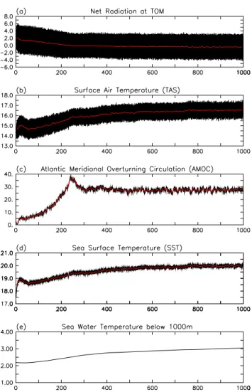
405 ppmv in the mid-Pliocene experiment, while other green-house concentrations are identical to the levels in the prein-dustrial simulation. The ocean model was started by adding the temperature anomalies between PRISM-3D dataset and LEVITUS data (Levitus and Boyer, 1994) to the initial field of the ocean temperature. The mid-Pliocene simulation has been integrated for 1000 yr. The short-wave radiation at the top of model (TOM) and surface air temperature (SAT) have reached equilibrium after a 500 yr spin-up (Fig. 1a, b). The strength of Atlantic Meridional Overturning Circulation (AMOC) reaches the maximum around 240 model yr and gradually evolves to a stable state (Fig. 1c). The trends of the SST and sea water potential temperature below 1000 m also become very small after several hundred simulated years (Fig. 1d, e). Therefore, the last 100 yr outputs of the mid-Pliocene simulation are used in this study for the climatology and compared to the PI experiment.
3 Model results
3.1 Changes in atmospheric climatology
3.1.1 Surface air temperature
The global annual mean SAT for mid-Pliocene is 16.59◦C
simulated with the FGOALS-g2, which is 4.17◦C warmer
relative to the PI simulation (Table 2). Such warming is larger than the PlioMIP ensemble mean of 8 AOGCMs of 2.66◦C
(Haywood et al., 2013), which is partly associated with the high equilibrium climate sensitivity (ECS – the equilibrium temperature response to a doubling of CO2) estimated from
Fig. 1.Time series from the mid-Pliocene simulation of
FGOALS-g2 for(a)the net short-wave radiation at the top of model (TOM,
W m−2);(b)surface air temperature (SAT,◦C);(c)the maximum of
Atlantic Meridional Overturning Circulation (AMOC, Sv);(d)sea
surface temperature (SST,◦C) and(e) the potential temperature
(◦C) averaged below 1000 m. The 10 yr running mean values of
each variable are shown in red curves in(a)–(d).
4.23 to 4.59◦C for the FGOALS-g2 model (Zheng and Yu,
2013). The pattern of annual mean SAT shows that the warm-ing is relatively small in the tropics, about 1–2◦C
Table 2.Global annual mean values for the atmospheric and oceanic variables in the preindustrial (0 ka) and mid-Pliocene (3 Ma) simulations. The values for Atlantic Meridional Overturning Circulation (AMOC) are estimated from the maximum stream function.
Net Radiation at TOM SAT Precipitation SST SSS AMOC
(W m−2) (◦C) (mm d−1) (◦C) (psu) (Sv)
0 ka –0.84 12.42 2.81 17.42 34.96 28.61
3 Ma –0.49 16.59 3.01 20.04 34.44 27.13
3 Ma–0 ka 0.35 4.17 0.2 2.62 –0.52 –1.48
The warming is amplified towards mid to high latitudes of both hemispheres, reaching a maximum over Greenland and Antarctica where the ice sheets are removed. The zonal mean shows that the warming is about 2◦C in the tropics and
increases to about 12 and 9◦C in the Northern and
South-ern hemispheres, respectively (Fig. 2b), which is within the range of the PlioMIP ensemble mean (Haywood et al., 2013).
3.1.2 Precipitation
The global annual mean precipitation increased 0.2 mm d−1
relative to the PI simulation (Table 2). The hydrological cycle in the tropics was strengthened in the mid-Pliocene as simu-lated by FGOALS-g2. Enhanced precipitation mainly occurs along the tropical Pacific, Indian Ocean, Indian and West African monsoon regions and mid to high latitudes while reduction of rainfall is observed in the subtropical regions in both hemispheres (Fig. 2c). The zonal mean shows that the annual mean precipitation increased about 0.76 mm d−1
around 10◦N and decreased by 0.18–0.36 mm d−1 around
30◦N and 10–30◦S, respectively (Fig. 2d). The precipitation
was greatly enhanced beyond 60◦S and 60◦N in both
hemi-spheres (Fig. 2d).
3.2 Changes in ocean mean states
3.2.1 SST and sea water potential temperature
The global annual mean SST was 2.62◦C warmer in the
mid-Pliocene relative to the PI simulation, where the entire ocean shows a SST warming with the maximums located over the North Pacific, East Antarctic and parts of the North Atlantic (Fig. 3a). The zonal mean of SST shows that the warming of the SST is no more than 5◦C between 40 and 65◦N (Fig. 3b),
implying that the warming is more pronounced over the land in the midlatitudes of the Northern Hemisphere (Fig. 2a). The warming along the Equator is fairly consistent across the Pa-cific, indicating that the zonal SST gradient remains similar to the PI simulation. Thus the permanent El Ni˜no-like con-dition as suggested by previous reconstruction studies (Wara et al., 2005) is not seen in the mid-Pliocene simulation by FGOALS-g2. The vertical profile of zonal mean sea water potential temperature also shows an entire warming from sur-face to deep ocean (Fig. 3c). Note that there is an extreme warming in the Arctic Basin in the mid-Pliocene simulation,
Fig. 2.The differences of annual mean values between the
mid-Pliocene and the preindustrial simulation (3 Ma–0 ka) for(a)SAT
(◦C);(b) zonal mean SAT (◦C);(c) precipitation (mm d−1), and
(d)zonal mean precipitation (mm d−1).
a bias caused by an inaccurate description of currents at the North Pole that resulted in the trapping of warm salty water in the Arctic Basin (Lin et al., 2013). Excluding the extreme warming in the Arctic Basin, the warming is relatively uni-form above 1500 m, and gradually decreases to a warming of 0.5◦C in the deep ocean (Fig. 3d).
3.2.2 Salinity
Fig. 3.The differences of annual mean values between the
mid-Pliocene and the preindustrial simulation (3 Ma–0 ka) for(a)SST;
(b)zonal mean SST;(c)the sea water potential temperature and
(d)zonal mean potential temperature, the red line is estimated by
excluding the changes north of 60◦N. Units:◦C.
inverse change relative to the changes in precipitation, de-creasing in the tropics and high latitudes and inde-creasing in the subtropical regions (Fig. 4b). The vertical profile shows that the salinity mainly increases below 1500 m in the ocean and the regions of North Atlantic Deep Water (Fig. 4c). The extreme salty water mass in the Arctic Basin and the fresh water above are related to the model bias affecting the po-tential temperature. Except for the Arctic bias, the salinity shows no significant change in the upper ocean and the in-crease in salinity is relatively uniform in the ocean below 1500 m (Fig. 4d).
3.2.3 AMOC
Most model simulations have predicted a weakened Atlantic Meridional Overturning Circulation in response to global warming (Molnar and Cane, 2002; Wara et al., 2005; Rav-elo et al., 2006). However, many studies have pointed to an enhanced AMOC to account for the reconstructions of relatively warm mid-Pliocene SST in the North Atlantic (Schmittner et al., 2005). In the mid-Pliocene simulation of FGOALS-g2, the maximum for AMOC reduces by 1.48 Sv (Table 2). The meridional profile shows that the overturning cell is shallower in the mid-Pliocene experiment (Fig. 5a–c). Thus the northward heat transport is reduced in the North Atlantic (Fig. 5d).
Fig. 4.Same as Fig. 3 but for the changes in salinity (psu).
Fig. 5.The stream function (Sv) for(a)preindustrial (0 ka) and(b)
mid-Pliocene (3 Ma) simulated by FGOALS-g2;(c)the difference
between mid-Pliocene and preindustrial (3 Ma–0 ka); and(d) the
northward heat transport (PW), black line is for the preindustrial and red line for the mid-Pliocene simulation.
3.3 Changes in the interannual variability
3.3.1 El Ni ˜no-Southern Oscillation (ENSO)
Fig. 6.The standard deviation of the SST anomalies over the
tropi-cal Pacific for(a)preindustrial (0 ka) and(b)mid-Pliocene (3 Ma);
(c)the time series of Ni˜no 3 index, black line is for the preindustrial
and red line for the mid-Pliocene simulation, the standard deviation
of the Ni˜no index is shown in brackets; and(d)same as(c)but for
the Ni˜no 3.4 index. Units:◦C.
reduced significantly by 35 % (PI: 0.74◦C; mid-Pliocene:
0.48◦C) in the mid-Pliocene (Fig. 6c), while the ENSO cycle
is slightly lengthened (PI: 3.3 yr; mid-Pliocene: 3.8 yr). The Ni˜no 3.4 index shows a similar reduction as shown in Fig. 6d. Although the changes in ENSO based on the proxy records and model simulations are not conclusive at present, the re-sults from FGOALS-g2 suggest that the ENSO simulation may be model dependent and associated with their different representation of the mean climate and air–sea coupling pro-cesses. In FGOALS-g2, the weakening of ENSO may be as-sociated with the weaker seasonal cycle of the SST in the eastern Pacific (not shown), which needs further analysis. 3.3.2 East Asian monsoon
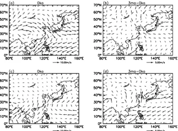
The simulation of FGOALS-g2 shows that the northerly winds weaken during boreal winter throughout the East Asian monsoon regions (Fig. 7b), while the stronger southerly winds related with the East Asian summer mon-soon prevail over eastern China (Fig. 7d). The stronger southerly winds are mainly associated with the stronger sub-tropical high located over the western Pacific. The southerly component of the Indian summer monsoon is somewhat weakened in the simulation. Both the weaker East Asian winter monsoon and stronger East Asian summer monsoon are attributed to the enhanced land–sea thermal contrast over East Asia, where the warming over land is larger than over the ocean (Fig. 2a).
Fig. 7.The atmospheric circulation at the 850 hpa for(a)East Asian
winter winds from preindustrial (0 ka);(b)the differences of the
winter winds between the mid-Pliocene and preindustrial
simula-tion (3 Ma–0 ka);(c)and(d)same as(a)and(b)but for the East
Asian summer winds. Units: m s−1.
4 Summary
In this study, we described the mid-Pliocene climate simu-lated by the FGOALS-g2. Compared to the PI simulation, the model results show that the global annual mean surface air temperature (SAT) was 4.17◦C warmer and the annual
precipitation increased by 0.2 mm d−1(Table 2). The model
[0,1)
[1,2) [3,4)
[2,3) >4 [-1,0)
[-2,-1) [-3,-2)
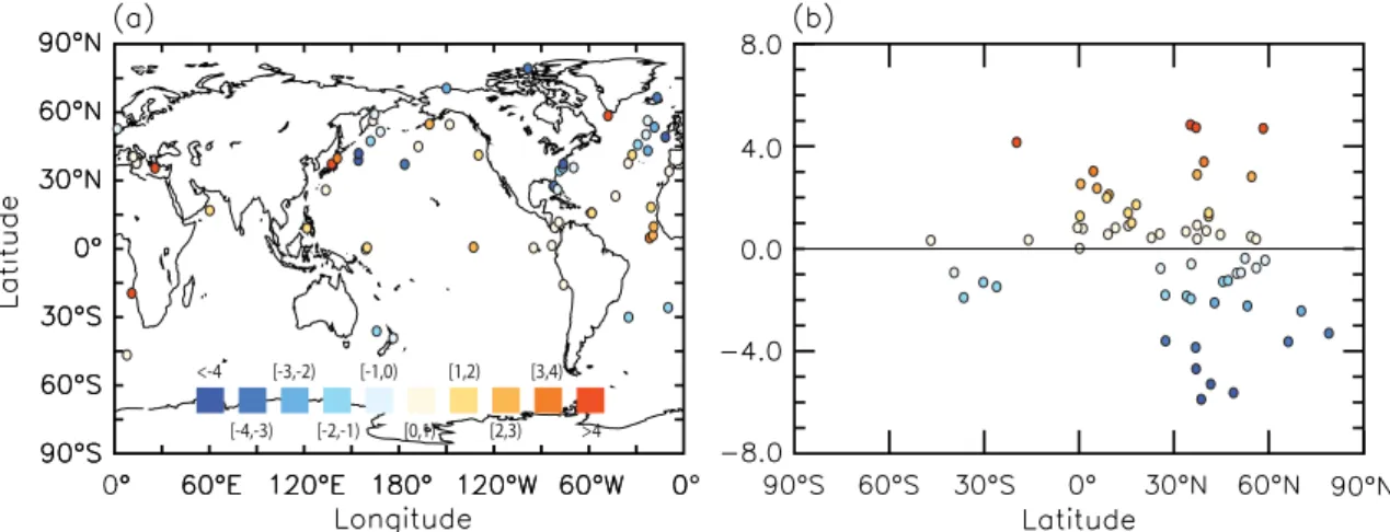
[-4,-3) <-4
Fig. 8. (a)Point-based data–model comparison of the sea surface temperature (model minus site data in◦C), and(b)the amount of data–
model discrepancy at each locality.
model shows a weakening of the interannual variability in the eastern tropical Pacific, in which the ENSO amplitude is significantly reduced and the ENSO cycle is slightly length-ened.
Despite this, FGOALS-g2 reproduced the basic climate features in the mid-Pliocene, the data–model biases are ob-served for the SST when compared to the PRISM3 SST re-construction (Dowsett et al., 2009). A total of 62 sites from the reconstruction are used for the comparison because they provide the reconstructed values for both the warm and cold months, and the annual mean SSTs are the means of February and August. Figure 8 shows the differences between model and site data, in which the simulated SSTs in mid-Pliocene broadly agree with the site data except for the larger data– model discrepancies located in the northwestern Pacific and the North Atlantic. In the North Atlantic, the SSTs are un-derestimated by the model at most of the drilling sites, which may be associated with the weaker northward heat trans-port in FGOALS-g2 (Fig. 5d). Such underestimation was also documented in Haywood et al. (2013) for other PlioMIP models. However, due to the uncertainties of the proxy re-construction, a better evaluation of the model simulation of the Pliocene requires efforts on both the sides of modelling groups and proxy reconstruction.
Acknowledgements. The authors thank the anonymous reviewers for their constructive comments that helped to improve the manuscript. This study was jointly supported by the Chinese National Basic Research Program (Grant Nos. 2010CB950502 and 2012CB955202), the National Natural Science Foundation (Grant Nos. 41006008 and 41023002) and the “Strategic Priority Research Program Climate Change: Carbon Budget and Relevant Issues” of the Chinese Academy of Sciences (Grant No. XDA05110301).
Edited by: D. Lunt
References
Contoux, C., Ramstein, G., and Jost, A.: Modelling the mid-Pliocene Warm Period climate with the IPSL coupled model and its atmospheric component LMDZ5A, Geosci. Model Dev., 5, 903–917, doi:10.5194/gmd-5-903-2012, 2012.
Craig, A. P., Jacob, R., Kauffman, B., Bettge, T., Larson, J., Ong, E., Ding, C., and He, Y.: CPL6: The new extensible, high per-formance parallel coupler for the Community Climate System Model, Int. J. High Perform. C., 19, 309–327, 2005.
Ding, Z. L., Yang, S. L., Sun, J. M., and Liu, T. S.: Iron geo-chemistry of loess and red clay deposits in the Chinese Loess Plateau and implications for long-term Asian monsoon evolu-tion in the last 7.0 Ma, Earth Planet. Sc. Lett., 185, 99–109, doi:10.1016/S0012-821X(00)00366-6, 2001.
Dolan, A. M., Haywood, A. M., Hill, D. J., Dowsett, H. J., Hunter, S. J., Lunt, D. J., and Pickering, S. J.: Sensitivity of Pliocene ice sheets to orbital forcing, Palaeogeogr. Palaeocl., 309, 98–110, doi:10.1016/j.palaeo.2011.03.030, 2011.
Dowsett, H., Robinson, M., Haywood, A., Salzmann, U., Hill, D., Sohl, L., Chandler, M., Williams, M., Foley, K., and Stoll, D.: The PRISM3D paleoenvironmental reconstruction, Stratigraphy, 7, 123–139, 2010.
Dowsett, H. J., Robinson, M. M., and Foley, K. M.: Pliocene three-dimensional global ocean temperature reconstruction, Clim. Past, 5, 769–783, doi:10.5194/cp-5-769-2009, 2009.
Dowsett, H. J., Robinson, M. M., Haywood, A. M., Hill, D. J., Dolan, A. M., Stoll, D. K., Chan, W.-L., Abe-Ouchi, A., Chan-dler, M. A., and Rosenbloom, N. A.: Assessing confidence in Pliocene sea surface temperatures to evaluate predictive models, Nature Climate Change, 2, 365–371, 2012.
Ge, J., Dai, Y., Zhang, Z., Zhao, D., Li, Q., Zhang, Y., Yi, L., Wu, H., Oldfield, F., and Guo, Z.: Major changes in East Asian climate in the mid-Pliocene: Triggered by the uplift of the Ti-betan Plateau or global cooling?, J. Asian Earth Sci., 69, 48–59, doi:10.1016/j.jseaes.2012.10.009, 2013.
Haywood, A. M., Dowsett, H. J., Otto-Bliesner, B., Chandler, M. A., Dolan, A. M., Hill, D. J., Lunt, D. J., Robinson, M. M., Rosen-bloom, N., Salzmann, U., and Sohl, L. E.: Pliocene Model Inter-comparison Project (PlioMIP): experimental design and bound-ary conditions (Experiment 1), Geosci. Model Dev., 3, 227–242, doi:10.5194/gmd-3-227-2010, 2010.
Haywood, A. M., Dowsett, H. J., Robinson, M. M., Stoll, D. K., Dolan, A. M., Lunt, D. J., Otto-Bliesner, B., and Chandler, M. A.: Pliocene Model Intercomparison Project (PlioMIP): experi-mental design and boundary conditions (Experiment 2), Geosci. Model Dev., 4, 571–577, doi:10.5194/gmd-4-571-2011, 2011. Haywood, A. M., Hill, D. J., Dolan, A. M., Otto-Bliesner, B. L.,
Bragg, F., Chan, W.-L., Chandler, M. A., Contoux, C., Dowsett, H. J., Jost, A., Kamae, Y., Lohmann, G., Lunt, D. J., Abe-Ouchi, A., Pickering, S. J., Ramstein, G., Rosenbloom, N. A., Salz-mann, U., Sohl, L., Stepanek, C., Ueda, H., Yan, Q., and Zhang, Z.: Large-scale features of Pliocene climate: results from the Pliocene Model Intercomparison Project, Clim. Past, 9, 191–209, doi:10.5194/cp-9-191-2013, 2013.
Jansen, E., Overpeck, J., Briffa, K. R., Duplessy, J.-C., Joos, F., Masson-Delmotte, V., Olago, D., Otto-Bliesner, B., Peltier, W. R., Rahmstorf, S., Ramesh, R., Raynaud, D., Rind, D., Solom-ina, O., Villalba, R., and Zhang, D.: Palaeoclimate, in: Cli-mate Change 2007: The Physical Science Basis, Contribution of Working Group I to the Fourth Assessment Report of the Inter-governmental Panel on Climate Change, edited by: Solomon, S., Qin, D., Manning, M., Chen, Z., Marquis, M., Averyt, K. B., Tig-nor, M., and Miller, H. L., Cambridge University Press, 433–497, 2007.
Jian, Z., Zhao, Q., Cheng, X., Wang, J., Wang, P., and Su, X.: Pliocene–Pleistocene stable isotope and paleoceanographic changes in the northern South China Sea, Palaeogeogr. Palaeocl., 193, 425–442, doi:10.1016/S0031-0182(03)00259-1, 2003. Jiang, H. and Ding, Z.: Eolian grain-size signature of the Sikouzi
lacustrine sediments (Chinese Loess Plateau): Implications for Neogene evolution of the East Asian winter monsoon, Geol. Soc. Am. Bull., 122, 843–854, doi:10.1130/b26583.1, 2010. Kamae, Y., Ueda, H., and Kitoh, A.: Hadley and Walker
Circula-tions in the Mid-Pliocene Warm Period Simulated by an Atmo-spheric General Circulation Model, J. Meteorol. Soc. Jpn., 89, 475–493, doi:10.2151/jmsj.2011-505, 2011.
Levitus, S. and Boyer, T. P.: World Ocean Atlas 1994, Vol. 4, Tem-perature, NOAA Atlas NESDIS 4, US Department of Commerce, Washington, DC, 117 pp., 1994.
Li, B., Wang, J., Huang, B., Li, Q., Jian, Z., Zhao, Q., Su, X., and Wang, P.: South China Sea surface water evolution over the last 12 Myr: A south-north comparison from Ocean Drilling Program Sites 1143 and 1146, Paleoceanography, 19, PA1009, doi:10.1029/2003PA000906, 2004.
Li, L., Lin, P., Yu, Y., Wang, B., Zhou, T., Liu, L., Liu, J., Bao, Q., Xu, S., Huang, W., Xia, k., Pu, Y., Dong, L., Shen, S., Liu, Y., Hu, N., Liu, M., Sun, W., Shi, X., Zheng, W., Wu, B., Song, M., Liu, H., Zhang, X., Wu, G., Xue, W., Huang, X., Yang, G., Song, Z., and Qiao, F.: The Flexible Global Ocean-Atmosphere-Land Sys-tem Model: Grid-point Version g2: FGOALS-g2, Adv. Atmos. Sci., 30, 543–560, doi:10.1007/s00376-012-2140-6, 2013a. Li, L., Wang, B., Dong, L., Liu, L., Shen, S., Hu, N., Sun, W., Wang,
Y., Huang, W., Shi, X., Pu, Y., and Yang, G.: Evaluation of Ver-sion Two of the Grid-point Atmospheric Model (GAMIL 2.0),
Adv. Atmos. Sci., 30, 855–867, doi:10.1007/s00376-013-2157-5, 2013b.
Lin, P. F., Yu, Y. Q., and Liu, H. L.: Oceanic Climatology in the Cou-pled Model FGOALS-g2: Improvements and Biases, Adv. At-mos. Sci., 30, 819–840, doi:10.1007/s00376-012-2137-1, 2013. Liu, H. L., Lin, P. F., Yu, Y. Q., and Zhang, X. H.: The baseline
eval-uation of LASG/IAP Climate system Ocean Model (LICOM) version 2.0, Acta Meteorol. Sin., 26, 318–329, 2012.
Lunt, D. J., Foster, G. L., Haywood, A. M., and Stone, E. J.: Late Pliocene Greenland glaciation controlled by a
de-cline in atmospheric CO2 levels, Nature, 454, 1102–1105,
doi:10.1038/nature07223, 2008.
Miller, K. G., Wright, J. D., Browning, J. V., Kulpecz, A., Kominz, M., Naish, T. R., Cramer, B. S., Rosenthal, Y., Peltier, W. R., and Sosdian, S.: High tide of the warm Pliocene: Implications of global sea level for Antarctic deglaciation, Geology, 40, 407– 410, 2012.
Molnar, P. and Cane, M. A.: El Ni˜no’s tropical climate and telecon-nections as a blueprint for pre-Ice Age climates, Paleoceanogra-phy, 17, 1021, doi:10.1029/2001pa000663, 2002.
Moran, K., Backman, J., Brinkhuis, H., Clemens, S. C., Cronin, T., Dickens, G. R., Eynaud, F., Gattacceca, J., Jakobsson, M., and Jordan, R. W.: The Cenozoic palaeoenvironment of the Arctic Ocean, Nature, 441, 601–605, 2006.
Naish, T., Powell, R., Levy, R., Wilson, G., Scherer, R., Talarico, F., Krissek, L., Niessen, F., Pompilio, M., Wilson, T., Carter, L., DeConto, R., Huybers, P., McKay, R., Pollard, D., Ross, J., Win-ter, D., Barrett, P., Browne, G., Cody, R., Cowan, E., Crampton, J., Dunbar, G., Dunbar, N., Florindo, F., Gebhardt, C., Graham, I., Hannah, M., Hansaraj, D., Harwood, D., Helling, D., Henrys, S., Hinnov, L., Kuhn, G., Kyle, P., Laufer, A., Maffioli, P., Ma-gens, D., Mandernack, K., McIntosh, W., Millan, C., Morin, R., Ohneiser, C., Paulsen, T., Persico, D., Raine, I., Reed, J., Riessel-man, C., Sagnotti, L., Schmitt, D., Sjunneskog, C., Strong, P., Ta-viani, M., Vogel, S., Wilch, T., and Williams, T.: Obliquity-paced Pliocene West Antarctic ice sheet oscillations, Nature, 458, 322– 328, doi:10.1038/nature07867, 2009.
Oleson, K. W., Dai, Y., Bonan, G., Bosilovich, M., Dickinson, R., Dirmeyer, P., Hoffman, F., Houser, P., Levis, S., and Niu, G.-Y.: Technical description of the community land model (CLM), Tech. Note NCAR/TN-461+STR, 2004.
Polyak, L., Alley, R. B., Andrews, J. T., Brigham-Grette, J., Cronin, T. M., Darby, D. A., Dyke, A. S., Fitzpatrick, J. J., Funder, S., and Holland, M.: History of sea ice in the Arctic, Quaternary Sci. Rev., 29, 1757–1778, 2010.
Ravelo, A. C., Dekens, P. S., and Mccarthy, M.: Evidence for El Nino-like conditions during the Pliocene, GSA Today, 16, 4–
11, doi:10.1130/1052-5173(2006)016<4:EFENLC>2.0.CO;2,
2006.
Raymo, M. E., Grant, B., Horowitz, M., and Rau, G. H.: Mid-Pliocene warmth: stronger greenhouse and stronger con-veyor, Mar. Micropaleontol., 27, 313–326, doi:10.1016/0377-8398(95)00048-8, 1996.
Rosenbloom, N. A., Otto-Bliesner, B. L., Brady, E. C., and Lawrence, P. J.: Simulating the mid-Pliocene Warm Period with the CCSM4 model, Geosci. Model Dev., 6, 549–561, doi:10.5194/gmd-6-549-2013, 2013.
comparison for the Middle Pliocene, Global Ecol. Biogeogr., 17, 432–447, doi:10.1111/J.1466-8238.2008.00381.X, 2008. Schmittner, A., Latif, M., and Schneider, B.: Model projections
of the North Atlantic thermohaline circulation for the 21st cen-tury assessed by observations, Geophys. Res. Lett., 32, L23710, doi:10.1029/2005GL024368, 2005.
Scroxton, N., Bonham, S. G., Rickaby, R. E. M., Lawrence, S. H. F., Hermoso, M., and Haywood, A. M.: Persistent El Ni˜no–Southern Oscillation variation during the Pliocene Epoch, Paleoceanogra-phy, 26, PA2215, doi:10.1029/2010PA002097, 2011.
Sun, D., Su, R., Bloemendal, J., and Lu, H.: Grain-size and accu-mulation rate records from Late Cenozoic aeolian sequences in northern China: Implications for variations in the East Asian win-ter monsoon and weswin-terly atmospheric circulation, Palaeogeogr. Palaeocl., 264, 39–53, doi:10.1016/j.palaeo.2008.03.011, 2008. Wan, S., Li, A., Clift, P. D., and Stuut, J.-B. W.: Development of the
East Asian monsoon: Mineralogical and sedimentologic records in the northern South China Sea since 20 Ma, Palaeogeogr. Palaeocl., 254, 561–582, doi:10.1016/j.palaeo.2007.07.009, 2007.
Wan, S., Tian, J., Steinke, S., Li, A., and Li, T.: Evolu-tion and variability of the East Asian summer monsoon dur-ing the Pliocene: Evidence from clay mineral records of the South China Sea, Palaeogeogr. Palaeocl., 293, 237–247, doi:10.1016/j.palaeo.2010.05.025, 2010.
Wang, B., Wan, H., Ji, Z. Z., Zhang, X., Yu, R. C., Yu, Y. Q., and Liu, H. L.: Design of a new dynamical core for global atmospheric models based on some efficient numerical methods, Science in China Series A: Mathematics, 47, 4–21, doi:10.1360/04za0001, 2004.
Wang, X. C., Liu, J. P., Yu, Y. Q., and Liu, H. L.: Experiment of cou-pling sea ice mode CICE4 to LASG/IAP climate system model, Chinese J. Atmos. Sci., 34, 780–792, 2010 (in Chinese).
Wara, M. W., Ravelo, A. C., and Delaney, M. L.: Permanent El Nino-like conditions during the Pliocene warm period, Science, 309, 758–761, doi:10.1126/Science.1112596, 2005.
Watanabe, T., Suzuki, A., Minobe, S., Kawashima, T., Kameo, K., Minoshima, K., Aguilar, Y. M., Wani, R., Kawahata, H., Sowa, K., Nagai, T., and Kase, T.: Permanent El Nino dur-ing the Pliocene warm period not supported by coral evidence, Nature, 471, 209–211, doi:10.1038/nature09777, supplementary available at: http://www.nature.com/nature/journal/v471/n7337/ extref/nature09777-s1.pdf, last access: 30 July 2013, 2011. Yan, Q., Zhang, Z. S., and Gao, Y. Q.: An East Asian Monsoon in
the Mid-Pliocene, Atmospheric and Oceanic Science Letters, 5, 449–454, 2012.
Yu, R. C.: A two-step shape-preserving advection scheme, Adv. At-mos. Sci., 11, 79–90, 1994.
Zhang, R., Yan, Q., Zhang, Z. S., Jiang, D., Otto-Bliesner, B. L., Haywood, A. M., Hill, D. J., Dolan, A. M., Stepanek, C., Lohmann, G., Contoux, C., Bragg, F., Chan, W.-L., Chandler, M. A., Jost, A., Kamae, Y., Abe-Ouchi, A., Ramstein, G., Rosen-bloom, N. A., Sohl, L., and Ueda, H.: East Asian monsoon cli-mate simulated in the PlioMIP, Clim. Past Discuss., 9, 1135– 1164, doi:10.5194/cpd-9-1135-2013, 2013a.
Zhang, Z., Nisancioglu, K. H., and Ninnemann, U. S.: In-creased ventilation of Antarctic deep water during the
warm mid-Pliocene, Nature Communications, 4, 1499,
doi:10.1038/ncomms2521, 2013b.
Zhang, Z. S., Yan, Q., Su, J. Z., and Gao, Y. Q.: Has the problem of a permanent El Ni˜no been resolved for the mid-Pliocene?, Atmos. Oceanic Sci. Lett., 5, 445–448, 2012.