Statistical modeling of fatigue crack growth rate in Inconel alloy 600
Kassim S. Al-Rubaie
a, Leonardo B. Godefroid
b,*, Jadir A.M. Lopes
caEMBRAER (Empresa Brasileira de Aerona´utica), Av. Brigadeiro Faria Lima 2170, 12227-901 Sa˜o Jose´ dos Campos, SP, Brazil bUniversidade Federal de Ouro Preto, Escola de Minas, Dept. de Engenharia Metalu´rgica e de Materiais,
Prac¸a Tiradentes 20, 35400-000 Ouro Preto, MG, Brazil
cCentro de Desenvolvimento da Tecnologia Nuclear – CDTN/CNEN Cidade Universita´ria, Pampulha, 30123-970 Belo Horizonte, MG, Brazil
Received 29 December 2005; received in revised form 24 July 2006; accepted 30 July 2006 Available online 26 September 2006
Abstract
Inconel alloy 600 is widely used in heat-treating industry, in chemical and food processing, in aeronautical industry, and in nuclear engineering. In this work, fatigue crack growth rate (FCGR) was evaluated in air and at room temperature under constant amplitude loading at a stress ratio of 0.1, using compact tension specimens. Collipriest and Priddle FCGR models were proposed to model the data. In addition, these models were modified to obtain a better fit to the data, especially in the near-threshold region. Akaike information criterion was used to select the candidate model that best approximates the real process given the data. The results showed that both Collipriest and Priddle models fit the FCGR data in a similar fashion. However, the Priddle model provided better fit than the Collipriest model. The modified Priddle model was found to be the most appropriate model for the data.
2006 Elsevier Ltd. All rights reserved.
Keywords: Inconel alloy 600; Fatigue crack growth rate; Statistical modeling; Nonlinear regression; Model selection; Akaike information criterion
1. Introduction
Inconel alloy 600 is a nickel–chromium–iron superalloy (Ni–Cr–Fe) that is widely used because of its good corro-sion and oxidation resistance[1–3]. This is a solid solution strengthened alloy, normally used in the annealed temper; the annealing treatment is dependent on properties required by the application. The alloy has good mechanical properties and presents the desirable combination of strength and toughness. The high nickel content of the alloy enables it to resist corrosion caused by many organic and inorganic compounds and also gives it high resistance to chloride ion stress corrosion cracking. The chromium content provides a resistance to sulfur compounds and to various oxidizing environments at high temperatures or in corrosive solutions[1,4].
Inconel alloy 600 is widely used in a variety of applica-tions. For its strength and corrosion resistance, it is used extensively in the chemical industry. Due to its strength and oxidation resistance at high temperatures, it is used for many applications in the heat-treating industry. In the aeronautical field, this alloy is used for a variety of engine and airframe components that must withstand high temperatures. Inconel alloy 600 is the standard material for construction of nuclear reactors. It has excellent resistance to high-purity water. Moreover, it is very resistant to chlo-ride ion stress corrosion cracking in reactor water systems
[5].
Tubes of a pressurized water reactor (PWR) steam gen-erator of a nuclear power plant represent the majority of the reactor coolant pressure boundary. The flow of cooling water with high velocity can cause cycling stresses (e.g. thermal cycling and vibration) in the tubes, generally made of Inconel alloys 600 and 690. The stresses may initiate and propagate fatigue cracks. In addition, aggressive service environments often accelerate the degradation rate. Exces-sive degradation may lead to failure of tubes and therefore
0142-1123/$ - see front matter 2006 Elsevier Ltd. All rights reserved.
doi:10.1016/j.ijfatigue.2006.07.013
* Corresponding author. Tel.: +55 31 3551 3012/3551 1586; fax: +55 31 3551 3012.
E-mail address:[email protected](L.B. Godefroid).
www.elsevier.com/locate/ijfatigue
International Journal of Fatigue 29 (2007) 931–940
implies reduced availability and safety of the entire plant
[6].
The objective of this study is to present and model FCGR data of Inconel alloy 600 at room temperature, since few works[7–10]have been published. Due to the sig-moidal shape of the log(da/dN)–log(DK) curve, Collipriest
[11,12] and Priddle [13] models were chosen to model the data. These models fit the entire FCGR curve. Nonlinear
statistical analysis [14,15] was done to estimate model
parameters. Akaike information criterion[16–19]was used
to select the most appropriate model to the data.
2. Experimental procedure
Inconel alloy 600 with a thickness of 7 mm was used.
The chemical composition is shown inTable 1.
Light microscopy was carried out on samples, polished
with 1lm diamond paste and electrochemically etched
with a solution of 10% phosphoric acid. Grain size mea-surement was done using a computerised image analysis. Vickers hardness test was performed with a load of 196
N for a time of 30 s. According to ASTM E8 [20], tensile
test was carried out with a rate of 2 mm/min using a 100 kN Instron machine.
FCGR test was conducted on pre-cracked compact
ten-sion specimens in accordance with ASTM E 647[21]. The
test was done under a constant amplitude sinusoidal wave
loading at a stress ratio (R) of 0.1 using a 100 kN MTS
servo-hydraulic machine, interfaced to a computer for machine control and data acquisition. The test was done at a frequency of 30 Hz under room temperature
condi-tions that ranged from 20C to 25C with a relative
humidity from 60% to 70% in air. The crack length was measured using a compliance method, in which a clip gauge is used to measure the elastic compliance of the spec-imen, which tends to increase with crack growth.
In addition, fatigue crack growth threshold (DKth) was
evaluated using a ‘‘load shedding’’ method proposed in
ASTM E647[21]. Basically, the test was conducted where
the stress intensity factor range (DK=KmaxKmin) was
decreased. Consequently, crack growth slowed down and the threshold was reached as the crack stopped growing, or reached a sufficiently low FCGR. According to ASTM
E647, DKth is about the DK corresponding to a FCGR
(da/dN) of 1010m/cycle.
Fracture toughness was evaluated by theR-curve deter-mination at room temperature and in air environment using compact tension specimens, in accordance with
ASTM E561[22]. Basically, cyclic loading was applied to
introduce a fatigue crack. As the crack reached the desired length, the fatigue cycling was stopped, and the load was
gradually increased until fracture occurred. The stress intensityKcis the value of KRat the instability condition
determined from the tangency point between the R-curve
and one of the appliedK-curves.
Fracture surfaces were analyzed in a JEOL scanning electron microscope.
3. Results and discussion
3.1. Microstructure and mechanical behaviour
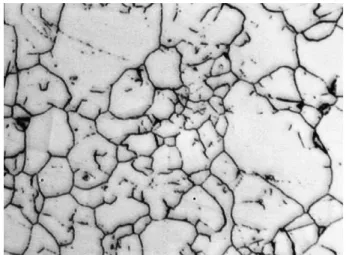
Fig. 1reveals the microstructure of the alloy with heter-ogeneous grains. The average grain size was determined as 14lm with a standard deviation of 9lm.
The results of the mechanical properties are presented in
Table 2. They met the specifications described in AMS 5540L[23].
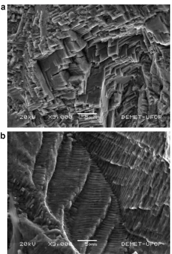
Fractographic analysis of tensile and fracture toughness specimens showed a transgranular and ductile fracture, with a mechanism of void nucleation, growth and coales-cence.Fig. 2shows this behaviour.
Fractographic analysis of fatigue crack growth at near-threshold shows a predominant transgranular fracture mode, with the ‘‘hill-and-valley’’ type appearance and shear facets, with an associated zig-zag path (Fig. 3a). Such fracture demonstrates high roughness and high crack deflection angles, characteristic of extensive crack closure induced by asperity wedging. At higher growth rates, frac-ture surfaces remain transgranular, but with evidence of striations (Fig. 3b).
Table 1
Chemical composition of Inconel alloy 600 (wt.%)
C S Fe Cr Ni
0.070 0.0007 9.46 13.92 70.12
Fig. 1. Microstructure of Inconel alloy 600, electrochemical etching, 10% phosphoric acid, (400·).
Table 2
Room temperature mechanical properties of Inconel alloy 600 rYS, MPa rTS, MPa e, % Hardness, HV Kc, MPapm DKth,
MPapm
386 687 33.5 224 40.08 6.38
3.2. FCGR modeling
3.2.1. FCGR models
The reason for building models is to link theoretical ideas with the observed data to provide a good prediction of future observations. Modeling of FCGR data has
enhanced the ability to create damage tolerant design
phi-losophies. Paris and Erdogan [24] proposed the most
important and popular work. They were the first who
cor-related FCGR with fracture mechanics parameters (Kmin
andKmax), describing the loading conditions in the region
of the crack front. They observed a linear relationship
between FCGR (da/dN) and DKwhen plotted on a log–
log scale. Paris and Erdogan proposed the power law relationship:
da
dN¼CDK
n
ð1Þ
where C and n are material parameters estimated from
experimental data.
The Paris–Erdogan equation does not consider: (a) the effect ofR, (b) the existence ofDKth, and (c) the accelerated
FCGR when the maximum stress intensity factor (Kmax)
approaches the fracture toughness (Kc). It does not
ade-quately describe FCGR regions I and III; it tends to over-estimate region I and underover-estimate region III. Although the Paris–Erdogan equation is a simplification of a very complex phenomenon, it is still very popular on account of significant engineering interest.
The typical curve of a log(da/dN)–log(DK), at a
pre-scribed condition (environment and R), is sigmoidal in
shape. It comprises three regions and is bounded at its extremes by DKthand DKc. In the intermediate region of
the curve, there is a linear relation between log(da/dN) and log(DK), as proposed by Paris and Erdogan.
Based on Eq.(1), many FCGR models have been
sug-gested to fit all or part of the sigmoidal curve. In this study, two models that fit all parts of FCGR curve are considered. These models are:
1. Collipriest model
Collipriest suggests the following inverse hyperbolic tan-gent function[11,12]:
da
dN ¼
CðKcDKthÞ
n 2
exp ln Kc
DKth
n2
tanh1ln
DK2
DKthKcð1RÞ
ln Kcð1RÞ
DKth
2
4
3
5 ð2Þ
where ln denotes the natural logarithm. 2. Priddle model
Priddle proposed the following function[13]: da
dN ¼C
DKDKth
KcKmax
n
ð3Þ
SinceDK=Kmax(1R), the model is given by
da
dN ¼C
DKð1RÞ DKthð1RÞ Kcð1RÞ DK
n
ð4Þ
Based on the results presented in [25], both Collipriest and Priddle models are modified by adding an extra param-eter (m) to obtain a better fit to the data, especially in the
Fig. 2. SEM fractography of toughness specimen of the Inconel alloy 600, 100·.
near-threshold region. The modified models are given respectively by Eqs.(5) and (6).
da
dN ¼
CðKcDKthÞ
n 2
exp ln Kc
DKth
n2
tanh1ln
DK2
DKthKcð1mRÞ
ln Kcð1RÞ
DKth
2
4
3
5 ð5Þ
da
dN ¼C
DKð1RÞ DKthð1mRÞ Kcð1RÞ DK
n
ð6Þ
3.2.2. Model fitting
Collipriest and Priddle models and their modifications are nonlinear regression models. A nonlinear model has at least one parameter (quantity to be estimated) that appears nonlinearly[14,15]. Nonlinear regression is an iter-ative procedure, and the basis used for estimating the unknown parameters is the criterion of least-squares. The fitting was carried out using a routine based on the
Marqu-ardt–Levenberg algorithm[26]. The fitting procedure
pro-vides: (i) parameters, (ii) error estimate on the parameter, and (iii) a statistical measure of goodness of fit.
The estimated parameters and the statistical properties
for FCGR models are presented in Tables 3 and 4. At
the 0.05 and 0.01 levels of significance, the estimated parameters are statistically significant, since their p-values
are smaller than the levels of significance.
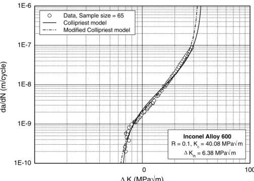
The experimental data and the estimated curves are shown inFigs. 4–6. The visual examination of these curves reveals that the modification in the Collipriest model pro-vides a better fit (Fig. 4). The same is also true for the case
of the modified Priddle model (Fig. 5). In addition, the
modified Priddle model provides a better fit than the mod-ified Collipriest (Fig. 6). It implies that the modified Priddle model offers the best approximation of the data.
3.2.3. Model validation
There are various graphical and numerical tools to assist goodness of fit of a model used with experimental data
[27,28]. The most common approach is to examine the residual. Three forms of graphical analysis were used. These are:
3.2.3.1. Measured–predicted plot.Plots of measured FCGR
against predictions of the underlying models are shown in
Fig. 7. The straight line gives values for measured = pre-dicted. An advantage of this type of plot is that the vertical deviations from the line are the actual residuals from the full fit. A residual is positive if the corresponding data point lies above the line and negative if the point lies below the line. Collipriest and Priddle models (Fig. 7a and b) behave in a similar fashion; it is hard to distinguish between them. The same is also true when the modified Collipriest and modified Priddle models are compared; however, the latter has relatively more support in the data, where the data points come close to the theoretical solid line.
3.2.3.2. Box plot.Box plot provides a graphical display of
data based on five-number summary (smallest value, lower quartile (Q1), median, upper quartile (Q3), and largest value). In box plot with a vertical orientation,Q1 and Q3 of the data are the lower and the upper lines of the box. The interquartile range (IQR) is the difference between
Table 3
Estimated parameters of FCGR models, Inconel alloy 600,R= 0.1
Model Parameter Estimate Std. error t-Value p-Value 95% LCL 95% UCL Collipriest C 5.609E12 7.023E13 7.987 3.76E11 4.206E12 7.012E12
n 2.621 4.809E02 54.508 <2E16 2.525 2.718
Priddle C 2.454E08 1.015E09 24.176 <2E16 2.252E08 2.657E08
n 1.151 2.034E02 56.60 <2E16 1.111 1.192
Modified Collipriest C 2.657E12 3.300E13 8.051 3.23E11 1.997E12 3.317E12
n 2.772 3.798E02 72.980 <2E16 2.696 2.848
m 2.301 1.892E01 12.161 <2E16 1.923 2.679
Modified Priddle C 2.425E08 7.425E10 32.658 <2E16 2.276E08 2.573E08
n 1.394 3.768E02 36.996 <2E16 1.318 1.469
m 2.463 2.592E01 9.506 1.02E13 1.945 2.981
Table 4
Statistical properties of FCGR models, Inconel alloy 600,R= 0.1
Model SSE SE MSE R2 R2
adj
Collipriest 0.63614 0.10049 0.01010 0.9792 0.9789
Priddle 0.59086 0.09684 0.00938 0.9807 0.9804
Modified Collipriest 0.34415 0.07450 0.00555 0.9887 0.9884
Modified Priddle 0.28036 0.06725 0.00452 0.9908 0.9905
SSE: sum of squares of error; SE: standard error of the residual; MSE: mean squared error;R2: coefficient of determination;R2
Q3 and Q1. The horizontal line within the box represents the median. The position of the median relative to theQ1 andQ3 gives information about the skewness in the middle half of the data. Whiskers are the dashed lines extended from the ends of the box to the adjacent values. The lower adjacent value is defined to be the smallest observation that is greater than or equal to theQ11.5·IRQ. The upper adjacent value is defined to be the largest observation that is less than or equal to theQ3 + 1.5·IRQ. Any
observa-tion falls outside the range of the two adjacent values is called an outlier. Notches in the box represent the robust confidence interval around the median and enable an examination of its variability.
Fig. 8shows side-by-side box plots of the residual data (measured–predicted) of the FCGR models. For all mod-els, the medians of the residuals are similar and nearly equal to zero. Residuals of the Collipriest and Priddle mod-els (Fig. 8a and b) seem to be similar; they appear to be
0 100
1E-10 1E-9 1E-8 1E-7 1E-6
Data, Sample size = 65 Collipriest model Modified Collipriest model
Inconel Alloy 600 R = 0.1, Kc = 40.08 MPa√m
∆K
th = 6.38 MPa√m
da/dN (m/cycle)
∆ K (MPa√m)
Fig. 4. FCGR curves of Inconel alloy 600,R= 0.1, comparison between Collipriest and modified Collipriest models.
1 10 100
1E-10 1E-9 1E-8 1E-7 1E-6
Inconel Alloy 600 R = 0.1, Kc = 40.08 MPa√m
Kth = 6.38 MPa√m Data, Sample size = 65
Priddle model Modified Priddle model
da/dN (m/
cycle)
∆K (MPa√m)
∆
1 10 100 1E-10
1E-9 1E-8 1E-7 1E-6
Inconel Alloy 600 R = 0.1, Kc = 40.08 MPa√m
∆Kth = 6.38 MPa√m Data, Sample size = 65
Modified Collipriest model Modified Priddle model
da/dN (m/cycle)
∆K (MPa√m)
Fig. 6. FCGR curves of Inconel alloy 600,R= 0.1, comparison between modified Collipriest and modified Priddle models.
-10.0 -9.3 -8.6 -7.9 -7.2 -6.5
-10.0 -9.3 -8.6 -7.9 -7.2 -6.5
Inconel Alloy 600 Priddle Model
-10.0 -9.3 -8.6 -7.9 -7.2 -6.5
-10.0 -9.3 -8.6 -7.9 -7.2 -6.5
Inconel Alloy 600 Collipriest Model
-10.0 -9.3 -8.6 -7.9 -7.2
-10.0 -9.3 -8.6 -7.9 -7.2 -6.5
Inconel Alloy 600 Modified Priddle Model
-10.0 -9.3 -8.6 -7.9 -7.2 -6.5
-10.0 -9.3 -8.6 -7.9 -7.2 -6.5
Inconel Alloy 600 Modified Collipriest Model
Measured log (da/dN), m/cycle
Predicted log (da/dN), m/cycle
-6.5
a
b
d
c
skewed to the right because the upper whisker is longer than the lower one. However, the Priddle model provides a slightly better fit to the data due to the smaller range of the upper whisker.
Box plots for the modified Collipriest and modified Prid-dle models (Fig. 8c and d) indicate that the distribution is symmetric because of the equal-sized whiskers and because the median line nearly lies in the middle of the box. On the other hand, the residual data have some extreme values
(outliers) as indicated by the (s) symbols. The extreme
negative values indicate that the estimated FCGR curve is conservative for the corresponding measured data points, as seen in Figs. 4 and 5.
The variability in residual data obtained from the mod-ified Collipriest appears much greater than that from the modified Priddle. This is due to the large range of the whis-kers and due to the longer length of the box (IQR). There-fore, it can be concluded that the modified Priddle model is the most approximating model to the data.
3.2.3.3. Normal quantile plot. Fig. 9 shows the normal
quantile plots (or normal probability plots) for the residu-als of the FCGR models. These plots are constructed by plotting the sorted values of the residual against the corre-sponding theoretical values from the standard normal distribution. The residuals of the Collipriest and Priddle models (Fig. 9a and b) appear to be skewed to the right, since the configuration seems to be a curve with slope increasing from left to right. Plots in Fig. 9(c) and (d) -0.3
-0.2 -0.1 0.0 0.1 0.2 0.3
d c
b a
Residual
FCGR Model
Fig. 8. Box plots for the residual data of FCGR models, Inconel alloy 600, R= 0.1, (a) Collipriest model, (b) Priddle model, (c) modified Collipriest model, and (d) modified Priddle model.
-2 -1 0 1 2
-0.2 -0.1 0.0 0.1
Inconel Alloy 600 Modified Collipriest Model
-2 -1 0 1 2
-0.3 -0.2 -0.1 0.0 0.1
Inconel Alloy 600 Modified Priddle Model
-2 -1 0 1 2
-0.1 0.0 0.1 0.2
Inconel Alloy 600 Priddle Model
-2 -1 0 1 2
-0.1 0.0 0.1 0.2 0.3
Inconel Alloy 600 Collipriest Model
Residual
Normal quantile
a
c
d
b
suggest that the residuals of the modified Collipriest and modified Priddle models appear to be normally distributed but contained a small number of outliers. The variability in the body of data for the modified Collipriest is greater than that for the modified Priddle model. Therefore, it may be concluded that the modified Priddle model is the most approximating model to the data.
To assess the model goodness of fit, several commonly used statistical numerical measures such as R2, R2
adj, SE,
and MSE are presented. TheR2statistic is a poor measure for model validation because adding an extra variable to a model will always increase R2even if the variable is com-pletely unrelated to the response variable. TheR2
adjstatistic
adjustsR2for the number of parameters in model. A model that maximizesR2
adjmay be chosen. Small values of SE and
MSE indicate that the model explains the data well.Table 4
suggests that the modified Collipriest and modified Priddle models (R2
adj0:99) are the best approximating models to
the data. However,Figs. 7–9demonstrated that the
modi-fied Priddle model provides relatively a better fit than the modified Collipriest.
3.2.4. Information-theoretic criteria and model selection
The least-squares criterion quantifies goodness of fit as the sum of squares of the vertical distances of the data points from the assumed model. That is, the best model for a particular data set is that with the smallest SSE. In fact, it is not simple to compare models with different parameters. The problem is that a more complex model (more parameters) gives more flexibility (more inflection points) for the curve being generated than the curve being defined by a simpler model (fewer parameters). Thereby, the SSE of a more complex model tends to be lower, irre-spective of whether the model is the most appropriate one for that data or not.
A model that is too simple cannot capture the regularity in the data; thereby, estimates will be far away from the unknown reality that generated the data (i.e. under-fitting or model bias). A model that is too complex tends to spread the data too thin over too many parameters, result-ing in a poor estimate of each parameter (i.e. over-fittresult-ing or model variance). It absorbs random noise more easily than a simple model. Simpler models have more bias but less variance; complex models have more variance but less bias
[29]. The best model, therefore, is one that provides the right balance between bias and variance. To achieve this, information-theoretic criteria proposed for model selection
may be used. Among the various criteria, Akaike Informa-tion Criterion (AIC) and Bayesian InformaInforma-tion Criterion (BIC) are widely accepted[16–19].
The AIC is an asymptotically unbiased estimator of the
expected Kullbach–Leibler (K–L) information [30] lost
when a model is used to approximate the underlying pro-cess (full reality) that generated the observed data. The
K–L information can be interpreted as a ‘‘distance’’
between full reality and a model. Thereby, the best model loses the least information relative to other models in the set. The AIC is given by
AIC¼ 2 lnðLÞ þ2K ð7Þ
whereLis the maximized likelihood andKis the number of estimated parameters in the model plus one (for estimated variance). The first term on the right-hand side represents a lack of fit measure, whereas the second term represents a model complexity measure. In the case of least-squares esti-mation, the AIC is given by
AIC¼Nln SSE
N
þ2K ð8Þ
whereNis the number of data points (sample size). When
more parameters are added to a model, the first term be-comes smaller, whereas the second term bebe-comes larger.
WhenNis small compared toKfor the highest
dimen-sioned model in the set of candidates (as a rough rule of thumb, N/K< 40), the use of AICC (Akaike Information
Criterion corrected for small samples) is recommended
[18]. The AICCis given by
AICC¼AICþ
2KðKþ1Þ
NK1 ð9Þ
where 2K(K+ 1)/(NK1) is a correction term. If Nis
much larger thanK, the numerator of the correction term
will be small compared to the denominator and the correc-tion will be tiny. In this case, the AIC or AICCmay be used
in model selection. For small samples, the correction is matter and the AICC will be used.
Models can only be compared using the AIC or AICC
when they have been fitted to exactly the same data set. Within the candidate models, a model minimizing the
AIC or AICCshould be selected to approximate the
under-lying process (truth). The use of the AICCrather than AIC
is preferred since it is more accurate for small samples and both are very similar for large samples.
Table 5
Model comparison, Inconel alloy 600,R= 0.1
Model K AIC AICC D L(MijD) W R2adj
Collipriest 3 294.737 294.356 50.993 8.45E12 8.44E12 0.9789
Priddle 3 299.536 299.156 46.193 9.32E11 9.30E11 0.9804
Modified Collipriest 4 332.669 332.025 13.324 1.28E03 0.001279 0.9884
Modified Priddle 4 345.994 345.349 0 1 0.9987 0.9905
A determination of the AICC differences (D) allows a
quick comparison and ranking of candidate models. For theith model, theDiis given by
Di¼AICCimin AICC ð10Þ
where min AICCis the smallest AICCamong all candidate
models. The D of the best approximating model thereby
equals zero, while the rest of the models have positive val-ues. The larger theDfor a model, the less probable is the best approximating model in the candidate set. As a rule of thumb[18], models withD62 have substantial support,
those with 36D67 have considerably less support, and
models withD> 10 have essentially no support.
The likelihood (L) of a model (Mi), given the data (D) is
LðMijDÞ ¼expð0
:5DiÞ ð11Þ
The likelihood of the best model equals unity (D= 0) and all other likelihoods are relative to the likelihood of the best model. The Akaike weight for the ith model (Wi) in
the set is given as the likelihood of the model divided by the sum of the likelihoods of all of the candidates. The
W may be interpreted as the ‘‘probability’’ that a model
is the best approximation to the reality, given the data. TheWfor the best model does not equal unity. The smaller is theW, the less plausible the model as the trueK–Lbest
model for the data. The evidence ratio of model i versus
model jis given by Wi/Wj; this is identical to the ratio of
likelihood of modelito that of modelj. The ratioWi/Wj
estimates how many times more support the data provide for modelithan model j[18].
If two models have similarWscores, but one uses many
more parameters than the other, the model with the fewest parameters will be selected. This is because both models fit about equally well, but the simpler is the more parsimoni-ous model.
The AIC can be used to compare both nested and non-nested models, whereas traditional likelihood ratio tests are valid only for nested models. The AIC was used to select the best model from the candidates available since these
are non-nested models.Table 5gives a comparison among
the fitting models. Since the modified Priddle shows AICC
score lower than those for the other models in the set, it is the closest model to the truth.
Based onR2
adjvalues,Table 5suggests that the modified
Collipriest and modified Priddle models (R2
adj0:99) are
the best approximating models to the data. However, an
examination of theDvalues shows that the modified
Colli-priest is very poor relative to the modified Priddle model.
Based on theWvalues, the modified Priddle model is 780
times more likely to be correct. Thereby, it may be con-cluded that the R2
adj is a poor statistical tool for model
selection.
4. Conclusions
Fatigue crack growth rate in Inconel alloy 600 was eval-uated in air and at room temperature under constant
amplitude loading at a stress ratio of 0.1, using compact tension specimens. Consequently, the collected data were modeled using Collipriest and Priddle models. In addition, these models were modified to obtain a better fit to the data, especially in the near-threshold region. Several com-monly used graphical plots and statistical numerical mea-sures were presented to assist the model goodness of fit.
The commonly usedR2
adjstatistic was found to be inefficient
for model selection. Then, Akaike information-theoretic criterion was used to select the candidate model that best approximates the real process given the data. The modified Priddle model was found to be the most appropriate model to the observed data.
References
[1] Friend WZ. Corrosion of nickel and nickel-base alloys. New York: Wiley; 1980.
[2] Inconel EL Alloy 600. Aerospace structural metals handbook, vol. IV, 1999.
[3] Crum JR. Major applications and corrosion performance of nickel alloys. In: Corrosion. ASM handbook, vol. 13. ASM; 1992. [4] Klarstrom DL. Characteristics of nickel and nickel-base alloys. In:
Corrosion. ASM handbook, vol. 13. ASM; 1992.
[5] Warke WR. Stress-corrosion cracking. In: Failure analysis and prevention. ASM handbook, vol. 11. ASM; 2002.
[6] Briceno DG, Hernandez AML, Marin MLC. Degradation of Inconel 600 MA steam generator tubes and potential replacement materials. Theor Appl Fract Mech 1994;21:59–71.
[7] James LA. Fatigue-crack propagation behaviour of Inconel 600. Int J Pressure Vessels Piping 1977;5:241–59.
[8] Brog TK, Jones JW, Was GS. Fatigue crack growth retardation inconel 600. Eng Fract Mech 1984;20:313–20.
[9] Damage tolerant design handbook, vol. 2, WL-TR-94-4053, 1994. [10] Park H-B, Kim Y-H, Lee B-W, Rheem K-S. Effect of heat treatment
on fatigue crack growth rate of Inconel 690 and Inconel 600. J Nucl Mater 1996;231:204–12.
[11] Collipriest JE. An experimentalist’s view of the surface flaw problem. ASME 1972:43–61.
[12] Collipriest JE, Ehret RM, Thatcher C. Fracture mechanics equations for cyclic growth. NASA technology utilization report, MFS-24447, 1973.
[13] Anderson TL. Fracture mechanics: fundamentals and applications. second ed. CRC Press; 1995.
[14] Ratkowsky DA. Nonlinear regression modeling: a unified practical approach. New York, NY: Marcel Dekker, Inc.; 1983.
[15] Bates DM, Watts DG. Nonlinear regression analysis and its applications. New York: Wiley; 1988.
[16] Akaike H. Information theory as an extension of the maximum likelihood principle. In: Petrov BN, Csaki F, editors. Proceeding of the Second International Symposium on Information Theory. Buda-pest: Akademiai Kiado; 1973. p. 267–81.
[17] Thelin T, Runeson P. Fault content estimations using extended curve fitting models and model selection. EASE’2000, 4th International Conference on Empirical Assessment & Evaluation in Software Engineering, Keele, England, 2000, pp. 77–96.
[18] Burnham KP, Anderson DR. Model selection and multimodel inference: a practical information-theoretic approach. second ed. Berlin: Springer; 2002.
[19] Posada D, Buckley TR. Model selection and model averaging in phylogenetics: advantages of Akaike information criterion and Bayesian approaches over likelihood ratio tests. Syst Biol 2004;53(5):793–808.
[21] ASTM E647. Standard test method for measurement of fatigue crack growth rates. Annual book of ASTM standards. ASTM; 2001. [22] ASTM E561. Standard practice forR-curve determination. Annual
book of ASTM standards. ASTM; 2001.
[23] AMS 5540L. Nickel alloy, corrosion and heat resistant, sheet, strip, and plate, 74Ni–15.5Cr–8.0Fe, annealed; 2000.
[24] Paris PC, Erdogan F. A critical analysis of crack propagation laws. J Basic Eng 1963(December):528–34.
[25] Rolfe ST, Barsom JM. Fracture and fatigue control in structures: application of fracture mechanics. Prentice-Hall, Inc.; 1977. p. 224.
[26] Marquardt DW. An algorithm for least squares estimation of parameters. J Soc Ind Appl Math 1963;11:431–41.
[27] Chambers JM, Cleveland WS, Kleiner B, Tukey PA. Graphical methods for data analysis. Duxbury Press; 1983.
[28] Devore JL, Farnum NR. Applied statistics for engineers and scientists. Duxbury Press; 1999.
[29] Pitt MA, Myung IJ. When a good fit can be bad. Trends Cognitive Sci 2002;6:421–5.