Numerical simulations of SAR microwave imaging of the Brazil current
surface front
This paper analyzes the hydrodynamic and
atmospheric instability modulation mechanisms
which inluence the Brazilian Current's (BC) thermal
front signature in Synthetic Aperture Radar (SAR)
images. Simulations were made using the M4S SAR
imaging model. Two SAR images of the Brazilian
Southeastern Coast depicting the BC's thermal front
were selected including a VV (ASAR/Envisat) and a
HH polarization (RADARSAT-1) image. Conditions
of current shear and divergence were reproduced for
the fronts imaged, using
in situ
(Acoustic Doppler
Current Proilers) current velocities. Wind velocity
ields were simulated based on QuikSCAT data.
Results showed that SAR imaging of the BC front
may be inluenced both by atmospheric instabilities
and hydrodynamic modulations. The irst
mechanism prevailed on the RADARSAT image
and the latter on the ASAR/Envisat image. When
atmospheric instabilities prevailed, the contribution
of shear and divergence was almost negligible.
When hydrodynamic modulations prevailed, a better
agreement between the simulated responses and
SAR image responses was obtained by inforcing a
reduction of 88% in the relaxation rate, and higher
divergence values, of the order of 10
-4s
-1. Results
indicate that, for some speciic cases, local increases
in shear and divergence may allow the detection of
the BC thermal front.
A
bstrAct
Carina Regina de Macedo*, João Antônio Lorenzzetti
Instituto Nacional de Pesquisas Espaciais - INPE.
(Av. dos Astronautas, 1758, CEP: 12227-010, São José dos Campos, SP, Brasil)
*Corresponding author: [email protected]
Financial Support: Coordenação de Aperfeiçoamento de Pessoal de Nível Superior (CAPES).
Descriptors:
Brazil Current front; Synthetic
Aperture Radars; SAR imaging model.
Esse artigo analisa os mecanismos, modulação
hidro-dinâmica e instabilidade atmosférica que permitem a
visualização da frente térmica da Corrente do Brasil
(CB) em imagens Radar de Abertura Sintética (SAR).
Simulações numéricas realizadas com o modelo M4S
basearam-se em duas imagens SAR da costa
sudes-te brasileira, nas polarizações VV (ASAR/Envisat) e
HH (RADARSAT-1), mostrando a região frontal da
CB. A simulação das condições médias de
cisalha-mento e divergência da região frontal se baseou em
dados
in situ
(
Acoustic Doppler Current Proilers
) de
correntes supericiais. Os campos de ventos foram
si-mulados a partir de dados do escaterômetro
QuikScat
.
Os resultados mostram que ambas as modulações por
instabilidade atmosférica e hidrodinâmica
inluencia-ram a visualização da frente da CB. O primeiro
me-canismo foi dominante na reprodução da modulação
da imagem RADARSAT, enquanto o segundo gerou
padrão próximo à imagem ASAR/Envisat. No caso de
dominância da instabilidade atmosférica, a inluência
da modulação hidrodinâmica foi pequena. Na
preva-lência de modulação hidrodinâmica, observou-se boa
concordância entre os resultados simulados e reais,
porém utilizando valores de divergência da ordem de
10
-4s
-1e impondo uma diminuição de 88% na taxa de
relaxação. Os resultados indicam que, em casos
es-pecíicos, o aumento da divergência/cisalhamento na
região frontal poderia possibilitar a visualização da
frente térmica da CB.
r
esumo
Descritores:
Frente da Corrente do Brasil, Radar
de Abertura Sintética, Modelo de imageamento
SAR.
INTRODUCTION
Ocean fronts are important oceanographic features related to which a wide array of physicochemical processes may be observed. Fronts are frequently zones of enhanced convergence and mixing where local hydrodynamics favor particle retention, while enrichment mechanisms allow the development of stable plankton communities (BAKUN, 2006). A spatial-temporal persistence of such primary production hotspots may, eventually, sustain important ishing stocks. Studies of ocean fronts also contribute to a better understanding of atmosphere-ocean interactions and ocean mesoscale variability (JOHANNESSEN et al., 2005).
Remote sensing can provide synoptic, high temporal coverage and high spatial resolution data of the ocean surface, aspects that stand as important elements for the study of ocean fronts. Sea Surface Temperature (SST) ields, obtained by thermal infrared radiometers, are often used to detect and map thermal fronts, while Chlorophyll-α ields may be used to detect local hydrodynamic retention and enrichment processes. Several studies using SST ields have recently been undertaken to characterize the variability of the Brazil Current (BC) surface front (SILVEIRA et al., 2008; LORENZZETTI et al., 2009).
As a limitation, both infrared and ocean color radiometers are passive sensors which depend on the emitted infrared or the relection of sunlight radiation, and are strongly inluenced by the concentration of water vapor in the atmosphere and the presence of clouds. In the case of ocean color sensors, imaging which is primarily done on the visible wavelength band is further limited to daylight time acquisitions. The detection of fronts using SST ields may also be hampered when a homogeneous thermal layer is developed above the frontal zone, concealing thermal contrasts. Though SST products from microwave radiometers are little inluenced by clouds and water vapor, their uses are still limited by coarse spatial resolutions, of scales of several kilometers, which often prevent a proper visualization of thermal fronts (LORENZZETTI et al., 2008). Despite such limitations, these products may still be employed in ocean front studies as complementary data.
Active remote sensing systems such as Scatterometers and Synthetic Aperture Radars (SAR) are capable of measuring changes in ocean surface roughness based on backscattering patterns, caused by Bragg waves (high frequency gravity-capillary resonant waves of the order of the radar’s wavelength), specular relection and
wave breaking. The relative inluences of each of these mechanisms vary with radar wave frequency, polarization and incidence angle (KUDRYAVTSEV et al., 2005). SAR sensors have been successfully employed in the detection of ocean fronts; frontal regions can be detected by SAR systems due to the changes in surface ocean roughness existing in these regions. SAR images have advantages over scatterometer data, as their high spatial resolution allows the representation of ine scales (of the order of a few to tens of meters), which are more appropriate to detect ocean fronts. There are three mechanisms that can be assumed to be responsible for most of the changes in ocean surface roughness in frontal zones and that strongly inluence the visualization of these features in SAR images (LYZENGA et al., 2004):
a) Interaction between surface waves and the surface current gradients, a mechanism also called hydrodynamic modulation. Changes in ocean surface roughness caused by the interaction between surface waves and strong gradients of current velocity ields - normally found in frontal zones - often lead to signiicant changes in the amount of backscattered radar energy. In regions of strong surface current convergences the Bragg wave energy is increased, enhancing radar backscattering, while in divergence zones, Bragg wave energy is decreased, leading to a reduction of the backscattered signal.
b) Concentration of surfactants in convergence zones. Convergence and divergence of surface currents inluence the horizontal redistribution and vertical accumulation of surfactants at the sea’s surface. Conditions of current convergence favor the development of surfactant accu-mulations. Surfactants tend to reduce radar backscattering (ROBINSON, 2004). In SAR images, the accumulation of surfactants is often represented by dark lines.
c) Instabilities of the atmospheric boundary layer (ABL), also known as ABL instability modulation. Signiicant changes in the SST ield, associated with the presence of thermal fronts, can inluence ocean-atmosphere heat exchanges. The ABL tends to be more stable on the cooler sides of the thermal fronts and the ABL is normally unstable and deeper in the warm sector of the front (CHELTON et al., 2004). These variations in ABL stability near the sea surface induce changes of the surface wind and stress as well as latent and sensible heat luxes (SMALL et al., 2008). Wind stress is the key variable controlling the short wind wave spectrum (Bragg spectrum) and consequently the Normalized Radar Cross Section - NRCS
on the two sides of the frontal zones are often signiicant enough to make them visible as interfaces separating the cold and the warm sides of the oceanic thermal front: cold SSTs are represented as darker areas, while brighter areas represent warmer SSTs (ROBINSON, 2004).
Few studies have used SAR images to investigate oceanographic features on the Brazilian Coast, especially for the detection of Brazil Current (BC) features such as eddies, meanders and fronts. RADARSAT-1 data (C-band) have been tested for the detection of the BC frontal zone in the Campos Basin on the southeastern coast of Brazil (LORENZZETTI et al., 2008). Despite some limitations, authors acknowledge the potential of those images as a complementary tool, along with SST imaging, for the detection of the BC front, emphasizing the real advantages under the presence of extensive cloud cover. Nonetheless, their results also show cases in which the CB front was clearly viewed in SST images but did not appear in near simultaneous SAR images.
It must be highlighted that the study of mesoscale features by SAR imaging may not be an easy task, even in the simplest cases. Such dificulties arise from the complex interactions between the physical processes inluencing the patterns of surface signatures in SAR images, along
with a generalized lack of in situ data matching SAR
acquisitions in space and time. Ideally, in situ data should
include surface wind speeds and directions, as well as a proper characterization of the ABL, along with other useful information such as the presence of surfactants (JOHANNESSEN et al., 2005).
Recent advances in the mathematical representations of the physical interactions between the electromagnetic radiation and the ocean surface also contemplate their representation in SAR images. These efforts have led to the development of mathematical numerical models that allow the simulation of SAR images. Direct models for SAR imaging simulation provide an alternative method for the study of the dynamics of mesoscale feature signatures in SAR images (JOHANNESSEN et al., 2005). The term “direct modelling” refers to a set of algebraic equations that provide estimates of the NRCS - a parameter that controls the brightness of SAR image pixels - in images of the ocean surface based on a series of sensor (frequency, polarization, incidence angles) and environmental (surface wind ields, wave spectra, surface currents and other) parameters.
Regarding the direct models, some publications address their development (ALPERS; HENNINGS, 1984;
ROMEISER; ALPERS,1997; ROMEISER et al., 1997; KUDRYAVTSEV et al., 2003a; KUDRYAVTSEV et al., 2003b and KUDRYAVTSEV et al., 2005) and others their use for SAR imaging simulations to study the dynamics of ocean surface features and their effects on SAR signatures (BRANDT et al., 1999; UFERMANN; ROMEISER et al., 2004; JOHANNESSEN et al., 2005). Recent models, such as the M4S and the Radar Imaging Model (RIM) are now able to provide very realistic simulation results. The present study employed the M4S model developed by ROMEISER and ALPERS (1997) ROMEISER et al. (1997), ROMEISER and THOMPSON (2000). This model is mostly based on the Bragg backscattering mechanism and the Weak Interaction theories (LONGUET-HIGGINS; STEWART, 1964; WHITHAM, 1965; BRETHERTON, 1971); it is also able to represent the geometric modulations caused by the tilt of illuminated facets and range variations, the hydrodynamic modulation of Bragg waves caused by longer waves, and it also includes the “velocity bunching” mechanism (ROMEISER et al., 1997). Details of the RIM model may be found in KUDRYAVTSEV et al. (2003a; 2003b; 2005), and in JOHANNESSEN et al. (2005). The RIM model also accounts for the modulation caused by surfactant accumulations and wave breaking at the frontal zone.
The objective of this study was to study the mechanisms inluencing the surface signatures of the BC front in the Campos Basin Region in SAR images. For that we conducted simulations using the M4S model, aiming to achieve a better understanding of the relative roles of environmental mechanisms (hydrodynamic modulation and ABL instabilities) in modulating the NRCS in the frontal zone.
MATERIAL AND METHODS
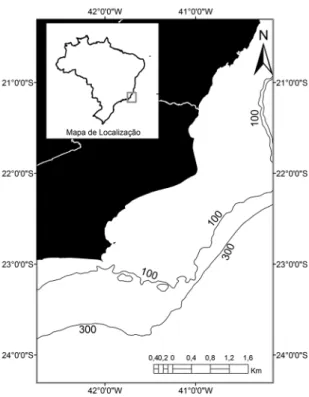
Study Area
The Campos Basin (Figure 1) is located on the Southeastern Brazilian Coast, between zonal limits of
20ºS and 25ºS. The region extends for 100,000 km2 and
encompasses a continental shelf width of 100 km. Shelf break depths vary from 80 m in its northern portion to 130 m in its southern portion. The continental slope extends
offshore for 40 km, with a mean declivity of 2º (VIANA
et al., 1998).
from a reanalysis (Level 4) of SST data acquired from both thermal and microwave radiometers (AQUA/AMSR-E, AQUA/MODIS, NOAA-18/AVHRR-3, TERRA/MODIS,
CORIOLIS/WINDSAT) along with in situ observations
(CHIN et al., 2013).
Both radar images were radiometrically calibrated (absolute calibration), providing comparable standardized values of the ocean surface radar signal backscattering. The original digital values for each pixel were converted into calibrated NRCS values. The ASAR/Envisat image calibration was conducted on Next ESA SAR Toolbox (NEST), using the algorithm proposed by ROSICH and MEADOWS (2004). The RADARSAT-1 image calibration
was performed by the PCI Geomatica 2013 software, using
the RADARSAT INTERNATIONAL (2004) method. Wind data consisted of daily products (level 2B) acquired by the SeaWinds scatterometer lying onboard the QuikSCAT satellite which was developed to provide oceanic wind speed and direction estimates, based on measurements of Bragg wave backscattering. The QuikSCAT satellite ended its operations in November 2009. The scatterometer wind ields employed here were reprocessed at NASA using the scatterometer geophysical model (v.3) developed by FORE et al. (2014). Wind speeds are assumed at 10 m height and under a condition of neutral atmospheric stratiication. QuikSCAT wind velocities were available on a 12.5 km pixel grid, at a spatial resolution of 25 km. As stated above, acquisition dates were chosen in order to coincide as far as possible with SAR acquisitions.
Values of divergence and shear of surface currents
on the BC front were calculated from in situ current
measurements acquired on a series of oceanographic
cruises (Comissões Oceano Sudeste - OCSE- II, IV e V;
Table 2) conducted by the Brazilian Navy in the study area. Proiles of current velocity and direction were obtained by Acoustic Doppler Current Proilers (ADCP) in different periods of the year. All data were processed at the Physical Oceanography Department of the Oceanographic Institute
of the University of São Paulo (Instituto Oceanográico/
Universidade de São Paulo - IO/USP), using the Common
Ocean Data Access System (CODAS) protocol, developed by the Hawaii University. Current velocities were available at a mean spatial resolution of 5.3 km. These
data are organized and may be foundin the archives of
the National Oceanographic Data Base (Banco Nacional
de Dados Oceanográicos - BNDO) maintained by the Brazilian Navy.
Figure 1. Map of the study area.
shedding between Cabo Frio and Cabo de São Tomé. SILVEIRA et al. (2004, 2008) associated the development of meanders and eddies to baroclinic instabilities caused by the intense vertical shear created by the contact between the southward surface low of the BC and the interior northward low of the Intermediate Contour Current (ICC) at depths of 500m.
Material
Figure 2. a) MUR SST ield acquired in the same date as the SAR acquisition. The black line represents the same transect depicted in the RADARSAT-1
image. b) RADARSAT-1 image acquired in November 21, 2005 (12:26 UTC). The black line represents a transect crossing the front, from where NRCS values were retrieved and compared to the simulated results. Lower NRCS values can be observed in the onshore sector of the black transect.
Figure 3. a) MUR SST ield acquired in the same date as the SAR acquisition. The black line represents the same transect depicted in the
ASAR/Envisat image. b) ASAR/Envisat image acquired in October 15, 2009 (12:32 UTC). The black line represents a transect crossing the front, from where NRCS values were retrieved and compared to the simulated results. Lower NRCS values delimit the center of the front.
Table 1. Acquisition information for the RADARSAT-1 and SAR/Envisat images analyzed.
Image
number Platform Date
Acquisition time (UTC)
Central Latitude
Central
Longitude Orbit
1 RADARSAT-1 21/11/2005 12:26:02 -22.215º -40.633 Descending
2 ASAR/Envisat 15/10/2009 12:32:06 -22.542º -42.250º Descending
Table 2. Summary of dates and seasons of ADCP data
acquisitions (OCSE - Comissões Oceanográicas Sudeste
II; IV and V).
Cruise Dates Seasons
OCSE-II 22/10/2002 to 03/12/2002 Spring OCSE-IV 28/01/2006 to 13/04/2006 Summer/Autumn OCSE-V 07/06/2010 to 07/07/2010 Winter
Methods
Shear and divergence of surface currents
at the BC front
Calculations of shear and divergence were based on the data acquired by the ADCP proiles sampled on the survey transects that covered the frontal zones depicted in both SAR images, between the localities of Arraial do Cabo and Cabo de São Tomé (Figure 1). One single transect crossing
the frontal zones was selected on each oceanographic cruise (Comissões OCSE II; IV and V). Calculations were made for the 20 m depth acoustic data, in which the inluence of spurious surface noise would be minimal.
Considering a horizontal plane x-y with the velocity
component u (v) in direction x (y), current shear (τ) and
divergence (Div) were calculated as indicated in equations
et al. (1997), along with the Limited Quadratic Source Function developed by WENSINK et al. (1999). The Limited Quadratic Source Function was chosen in order to limit the wave height decay in zones under low wind speeds. Wave breaking effects were not considered, as the proper parameterizations are still under development in the M4S model. The simulations were conigured by input iles so that the second module (M4Sr320) used the wave spectrum produced by the M4Sw320 module, along with sensor (frequency, polarization, platform altitude and velocity) and imaging (incidence angle, look direction, and platform heading) attributes, to compute NRSC matrices. This module, also known as the Radar Module, also incorporates the contributions from the Improved Composite Surface Model (ROMEISER & ALPERS, 1997; ROMEISER et al., 1997; ROMEISER; THOMPSON, 2000), as well as from artifacts generated by the imaging mechanism. The M4S modelling procedures are summarized in Figure 4.
Figure 4. Flux diagram depicting the M4S modelling scheme.
In this study, directions x and y were chosen
with reference to the orientation of the thermal front.
The x-direction is chosen as normal to the front, and
consequently the y-direction runs parallel to the front.
Since the sampling transects used in the analysis were always orthogonal to the thermal front orientation, the second terms of Equations 1 and 2 were neglected during shear and divergence calculations.
Maximum values for shear and divergence obtained
from available in situ data were selected and averaged
for each transect, on each survey cruise. Mean shear/ divergence maxima were treated here as the typical values of shear and divergence found in the BC frontal zone.
We found typical values of divergence of ±3 × 10⁻⁵s-1,
while typical shear was -4 × 10⁻⁵s-1. Such values were,
then, employed as inputs in the M4S simulations in the following stages of this study.
M4S - The Numerical Model to simulate
SAR microwave ocean imaging
In order to simulate SAR images representing the BC ocean fronts, we employed the M4S ocean surface microwave interaction model. The theoretical basis of the M4S model is presented in ROMEISER et al. (1997), ROMEISER and ALPERS (1997), and ROMEISER and THOMPSON (2000). The M4S model employs a set of numerical routines that simulate microwave radar imaging of ocean surface features that may be either associated with or modulated by a surface current ield, as well as by variations of the ocean surface wind ield. The inherent variability of current and wind ields through the hydrodynamic and aerodynamic modulation mechanisms can modulate the surface wave spectrum and modify the NRCS values observed in SAR images. The M4S model can be used to simulate SAR images of the ocean surface acquired on different frequency bands, polarizations and incidence angles. The model’s applicability is for incidence angles between 20º and 70º (Bragg wave range).
Simulations with the M4S model require two mandatory input iles containing the velocity ields for surface currents and 10 m height winds. While ocean bathymetry and NRCS values in the continent or island regions may also be used, our simulations were processed using only the mandatory inputs iles. The M4S irst module (M4Sw320) calculates a spatially varying wave height spectrum based on the surface current and wind velocity ields. For this stage, we employed the wave height spectrum model developed by ELFOUHAILY
SAR Microwave simulations at the BC front
The inluence of the hydrodynamic modulation mechanism on NRCS values at the BC frontal zone was evaluated through a series of customized simulation experiments with the M4S model. The irst objective of these experiments was to evaluate the response of the NRCS values to variations in surface current shear in the frontal zone. As a second objective, we evaluated the model response to surface current divergence/ convergence, which are common features in ocean fronts. To generate the surface current velocity ield iles needed as M4S model inputs we constructed synthetic current ields using the typical values of shear anddivergence derived from in situ ADCP data. To obtain
The center of the front differed for each image: for the RADARSAT-1 image, 12,500 m, while for the ASAR/ ENVISAT image, 18,500 m. The origin of the x-axis is at the left end of each transect. An incidence angle of 24.8º was calculated for the BC front depicted by Image 1. A lower value, of 18.9º, was present at the front depicted by Image 2. Considering that the M4S model only accepts incidence angles of more than 20º, all of our simulations assumed ixed angles of 20º for image 2.
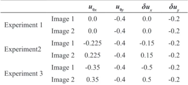
Table 3. Parameters of mathematical relationships proposed by Askari et al. (1997) used to obtain the chosen shear and divergence for each experiment.
u0x u0y δux δuy
Experiment 1 Image 1 0.0 -0.4 0.0 -0.2
Image 2 0.0 -0.4 0.0 -0.2
Experiment2 Image 1 -0.225 -0.4 -0.15 -0.2 Image 2 0.225 -0.4 0.15 -0.2
Experiment 3 Image 1 -0.35 -0.4 -0.5 -0.2
Image 2 0.35 -0.4 0.5 -0.2
Where ux and uy represent the current velocity
components normal and parallel to the ocean front,
respectively. The terms u0 and δu are constants representing,
respectively, the mean and the variations on current velocity; xc represents the location of the front along the x axis and δxc is the spatial extension (m) where current
velocity variations occur.
In order to better understand the effects of hydrodynamic modulation, three different experiments were conducted. The irst experiment considered only the effects caused by current shear. The second and third experiments considered the effects caused by current shear and divergence, changing the magnitude of the divergence. These experiments were done twice; one group for Radarsat-1 and the other for Envisat SAR images. All simulations were structured so as to reproduce the environmental characteristics and imaging patterns on both SAR images.
All simulations assumed a typical shear value of
-4 × 10⁻⁵s-1. The behavior of the NRCS values at the BC frontal
zone was signiicantly different on the two SAR images. For the RADARSAT-1 image (Image 1) (Figure 2) they change from a lower value at the shelf to a higher value across the front and at BC. In the ASAR/ENVISAT image (Image 2) (Figure 3), the NRCS values show a negative anomaly at the frontal region. For the second type experiments, we assumed
negative divergence (convergence) values of -3 × 10⁻⁵s-1 for
Image 1, and a positive value of 3 × 10⁻⁵s-1 for Image 2.
It must be noted that the divergence values used here
had magnitudes of the order of 10-5s-1. Similar studies
of frontal zones (UFERMANN; ROMEISER, 1999; KUDRYAVTSEV et al., 2005) have often assumed mean
divergences of higher magnitudes (10-4s-1). Considering
that our estimates of shear and divergence were based on
in situ measurements on dates differing from our SAR
acquisitions and that the spatial resolution of the ADCP data available could be underestimating the real current changes at the front, we decided to conduct a third type of experiment, in which mean divergence was increased by one order of magnitude. Therefore, we assumed a negative
divergence of -1 × 10⁻⁴s-1 for Image 1, while assuming a
positive divergence of 1 × 10⁻⁴s-1 for Image 2.
Table 3 presents a summary of the parameters employed in each experiment. Following LORENZZETTI
et al. (2009), a spatial extension of 5 × 10³ m was assumed
as the BC front width where velocity variations occurred.
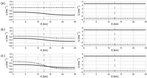
All experiments designed for studying the shear and divergence effects were carried out using constant and homogeneous synthetic wind ields. As the main objective of the experiments was to evaluate the effects of hydrodynamic modulation over the SAR signatures of the BC ocean front, the use of homogeneous wind ields was necessary in order to reduce the inluence of wind speed variability on the results. Mean wind speeds (Umean) were determined using SeaWinds scatterometer data as close as possible to the SAR imaging times. Maximum time difference was 7 hours for image 1. An information summary of the wind parameters used to build the synthetic wind ields is presented in Table 4. Figures 5 and 6 represent the synthetic wind and current ields used as inputs in the Experiments related to Images 1 and 2, respectively. Graphics depict the variations in current (left) and wind (right) velocities along a transect normal to the BC front.
Figure 5. Representations of the synthetic ields used as inputs in the Experiments related to Image 1: variations of
surface current (left) and wind (right) velocities represented along a transect crossing the BC front. Vertical gray lines mark the center of the front (xc): the areas at the left side represent the continental shelf region, while the right side is associated to the BC area. a) Experiment 1: surface current ields assuming a shear of -4 × 10⁻⁵ s-1, and
an homogeneous wind ield; b) Experiment 2: current ields assuming divergence of -3 × 10⁻⁵ s-1, and a shear of
-4 × 10⁻⁵ s-1, with a homogeneous wind ield; c) Experiment 3: current ields assuming a divergence of -1 × 10⁻⁴ s-1
and a shear of -4 × 10⁻⁵ s-1, with an homogeneous wind ield. Dashed black lines represent the velocity components
normal to the front; solid black lines represent the velocity components parallel to the front. Table 4. Information summary for the Wind data used to
build the synthetic Wind ields used in the experiments. Mean wind speeds (Umean) were retrieved from wind velocity ields
acquired by SeaWinds near the SAR imaging times. Wind directions assume a clockwise direction from a geographic north (α), and a counterclockwise direction from the x axis (β), normal to the front axis. φ wind directions consider the wind origin, assuming a counterclockwise direction, in relation to the radar beam (look direction). Ux and Uy represent the
speed components perpendicular and parallel to the BC front, respectively.
Image α (°) β (°) φ (°) Umean (ms-1)
Ux (ms-1)
Uy (ms-1)
1* 148 124 131 5.84 -3.26 4.84
2** 39 273 240 7.42 0.39 -7.41
* RADARSAT; ** Envisat.
Over warmer waters, ABL instability and surface wind increases through enhanced vertical mixing; over colder waters, wind stress and surface winds decrease in association with increased stability. Changes in wind stress are mostly attributable to SST-induced changes in wind speed (CHELTON; XIE, 2010). In the M4S model
the neutral stability wind speed at 10 m height (U10) is the
only parameter which represents the effect of the wind ield on the ocean wave spectrum. The effect of variations of atmospheric stability is normally represented by variation
of the friction velocity or the drag coeficient. Since the variations of the drag coeficient are not accounted for in the model, only variations in the wind speed on the two sides of the front can be used under the assumption of a constant drag coeficient (UFERMANN; ROMEISER, 1999). Thus, the second group of experiments, speciically designed for studying the ABL instability change in the frontal zone, employed spatially varying synthetic wind ields. Variations of wind speeds were represented using the methodology used by UFERMANN and ROMEISER (1999). This method calculates wind speeds at frontal zones using a series of M4S simulations, and evaluating the increasing trends observed in the NRCS ields.
Variations on the NRCS across the front depicted in Image 1 were calculated by selecting 11 transects orthogonal to the ocean front. In order to reduce the effects from speckle noise - an intrinsic high frequency noise present in SAR images- a single typical transect was created by calculating the medians from the 11 transects at each point of it. This median transect was further averaged using a ive pixel window ilter.
Figure 6. Same as Figure 5, considering the experiments related to Image 2. a) Experiment 1: surface current
ields assuming a shear of -4 × 10⁻⁵ s-1, and an homogeneous wind ield; b) Experiment 2: current ields assuming
divergence of 3 × 10⁻⁵ s-1, and a shear of -4 × 10⁻⁵ s-1, with an homogeneous wind ield; c) Experiment 3: current
ields with a divergence of 1 × 10⁻⁴ s-1 and a shear of -4 × 10⁻⁵ s-1, with an homogeneous wind ield. Dashed black
lines represent the velocity components normal to the front; solid black lines represent the velocity components parallel to the front.
Figure 7. Box plot comparing the NRCS values at the inside
(offshore) zones and outside (onshore) zones of the front. NRCS are plotted in dB (10*log10 NCRCS) scale. The horizontal line inside the boxes represent the median value.
through the transect values. The NRCS values were, in the sequence, separated according to their position in relation to the BC front, generating two groups of pixels: inside pixels are located offshore of the front and outside ones onshore (towards the coast). Both groups of values are well distinguishable, as depicted in Figure 7, attesting the presence of aerodynamic modulation. The mean NRCS was of -9.5 dB for outside values, and of -7.3 dB for inside values, yielding a mean difference of 2.2 dB. For the Gulf Current front, UFERMANN and ROMEISER (1999) found a smaller difference, of 1.4 dB, using SIR-C/X-SAR images (C band; 5.3 GHz) with VV polarizations.
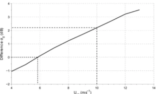
The mean difference of 2.2 dB observed in the frontal region was converted into wind speed variation, using M4S simulations. In order to obtain a reference proile representing the increase of NRCS values with wind speed, a series of 10 different M4S simulations were conducted, using 10 homogeneous wind ields of different speeds and a null
current ield. Wind ields with increasing speeds, from 4 ms-1
to 13 ms-1, at increments of 1 ms-1for each new simulation
were used. All simulations considered the imaging attributes of Image 1, such as: same polarization, mean incidence angle, azimuthal angle between wind direction and orientation of the front, as well as satellite sensor speciics.
Taking the mean wind speed of the study area
from QuikSCAT data (5.84 ms-1) as reference, which
corresponded to a NRCS of -12.21 dB, we plotted the NRCS differences from it for each simulation as a function of used wind speed (Figure 8). Thus, the zero value on the y axis corresponds to a simulated NRSC associated
with the mean wind speed of 5.84 ms-1. Regarding the
graphic analysis, an increment of 2.2 dB across the front, as observed in the RADARSAT-1 image, would indicate
an increase of 4.16 ms-1 in wind speeds (from 5.84 ms-1 to
Figure 8. Difference between simulated NRCS values obtained by
the M4S under varying homogeneous winds and that of the Reference proile versus wind speed. The black dashed line represents the NRCS
value for the mean wind intensity at the study area (5.84 ms-1); the
dash-dot line represents the wind intensity estimate when considering the increase in the NRCS at the BC front.
The spatially varying synthetic wind ields were then parameterized using the same method used in the parameterization of the surface current ields. Wind
gradients were also decomposed into normal (Ux) and
parallel (Uy) components (assuming the front as reference).
Where the constants U0 and δU represent the mean
wind speed and its variation at 10 m height, assuming a
neutral atmospheric stratiication. xw is the location of the
wind front along the x axis, while δxw is the width (m)
along which wind velocity changes occur.
An angle of 124º was assumed between the wind
direction and the x axis (See βvalue in Table 4). Hence,
the normal component Ux varied from -3.26 ms-1 to -5.59
ms-1, while the parallel component varied from 4.84 ms-1
to 8.29 ms-1. In such cases, we adopted mean wind speed
components of U0x = 4.43 ms-1 and U0y = 6.57 ms-1, while
the variations in wind components were of -2.33 ms-1 and
3.45 ms-1. A width of 5 × 10³ m was deined. Front locations
were centered at 12,500 m in the RADARSAT-1 Image. These simulations employed null current ields in order to reduce the inluence of current variability, since the main objective of the experiments was to evaluate the effects of aerodynamic modulation over the SAR signatures of the BC ocean front.
The experiments carried out in the sequence also incorporated the effects from shear and divergence, by using parameterized current ields, as had been done previously for the hydrodynamic modulation experiments. In the irst experiment for variable winds, we added a negative divergence of -3 × 10⁻⁵s-1, and a shear of -4 × 10⁻⁵ s-1.
In the second experiment, divergence was increased by one
order of magnitude (-1 × 10⁻⁴s-1), while shear remained
the same as in the previous experiment. Representations of the wind and current ields used as inputs on the ABL instability Experiments are summarized by the graphics of Figure 9.
All Experiments described in this section were repeated, now using a modiied relaxation rate, obtained by multiplying the original magnitude by a factor of 0.12. Such a procedure was suggested by BRANDT et al. (1999) in order to obtain better signal modulations to simulate the effects of solitary waves in SAR images.
Analysis of Results
Results were evaluated and interpreted based on a quantiication of the NRCS modulations for both real (SAR Images) and simulated (Experiments) frontal zones. As before, calculations were based on 11 transects perpendicular to the thermal front, from which real NRCS values were retrieved. Transect sizes differed for RADARSAT (12.5 km) and ASAR/ENVISAT (37.5 km) images due to their different pixel size (spatial resolution). To reduce the speckle noise present on each transect, a median NRCS from the 11 transects was calculated which was then iltered using a 5 pixel window. As a inal step, we removed the decaying effect related to variations on the radar incidence angles. The speckle noise reduction process was only applied to real images. Finally, the linear NRCS modulation was transformed into a dB scale, using
Where σ0i is the NRCS value at each point (i) of the
transect, and σ0mean is the mean NRCS at the outside sector
of the front (in this case the outer shelf region of the continental shelf).
RESULTS
Figure 9. Representation of the synthetic current (left) and wind (right) ields employed as inputs on the
Experiments for Image 1. Graphics depict current and wind velocity variations along an imaginary transect crossing the BC front. Vertical gray lines mark the center of the front (xc): the areas at the left side represent
the continental shelf area, while the right side represent the BC area. a) Experiment 1: null current ield with a spatially varying wind ield; b) Experiment 2: spatially varying wind ield and current ield assuming a divergence of -3 × 10⁻⁵ s-1, and a shear of -4 × 10⁻⁵ s-1; c) Experiment 3: spatially varying wind ield and current ield assuming
a divergence of 1 × 10⁻⁴ s-1 and a shear of -4 × 10⁻⁵ s-1. Dashed black lines represent the velocity components normal
to the front; solid black lines represent the velocity components parallel to the front.
Figure 10. Results from simulation experiments related to Image 1 (RADARSAT-1, solid black lines), without
modifying the original relaxation rates. Graphics represent sections of relative NRCS (vertical axis) along a normal transect crossing the BC front: a) Considering the effect of shear (-4 × 10⁻⁵ s-1) alone (dashed black line), while
assuming an homogeneous wind ield (5.84 ms-1); b) Considering the effects of shear and divergence values of -3 ×
10-5 s-1 (dashed black line), and -1 × 10⁻⁴ s-1 (gray line), while assuming an homogeneous wind ield; c) Considering
the effects of a spatially varying wind ield (5.84 ms-1 to 10 ms-1, assuming a direction ∅ = 131º) (dashed black
line); d) Considering the effects of shear and divergence values of -3 × 10⁻⁵ s-1 (dashed black line), and -1 × 10⁻⁴ s-1
(gray line), while assuming a spatially varying wind ield.
depicting a step-like pattern: colder waters in the inner sector of the continental shelf are characterized by lower values of relative NRCS, while higher values are related to the warmer BC waters, found offshore of the front. Maximum modulation was of approximately 3.5 dB, when ignoring the effects caused by speckle noise.
Figure 11. Same as Figure 10, considering an eighty-eight percent reduction of the relaxation rates.
When considering both shear and divergence
(-3 × 10⁻⁵s-1), the simulated NRCS modulation across the
front was again low when compared to the observed one in the original image (Figures 10b and 11b, dashed black line). The NRCS changes on the transect were characterized by a peak at the front (+0.05 dB modulation for simulation with no relaxation rate changes and +0.15 dB for relaxation modiied), dropping to negative modulations of NRCS in
the inside BC region. Themodulation was higher when
compared to the results from the previous experiment (having only a current shear), but were still well below the image benchmarks. With the inclusion of a higher
divergence (-1 × 10⁻⁴s-1), maximum modulations reached
approximately 0.30 dB (no relaxation rate changes) and 0.85 dB (relaxation modiied) with similar spatial patterns of NRCS modulations in both simulated results (no changing/changing the relaxation rate) and previous simulation (Figures 10b and 11b, gray line).
The experiments evaluating only the effects of ABL instabilities also produced step-like modulation patterns (Figures 10c and 11c). This time, simulated modulations were closer to those of the image, reaching +2.26 dB with unadjusted relaxation rates, and +2.39 dB with modiied relaxation rates. When considering the ABL instabilities,
with current shear (-4 × 10⁻⁵ s-1) and divergence
(-3 × 10⁻⁵s-1) (Figures 10d and 11d, dashed black line),
simulated modulations appeared as a step-like pattern, reaching +2.26 dB in the unadjusted case, and +2.37 dB in the decreased relaxation case. The insertion of a higher
divergence (-1 × 10⁻⁴s-1) (Figures 10d and 11d, gray line)
resulted in a step-like pattern and a lower modulation (+2.04 dB) for unadjusted relaxation rates. When the
relaxation rates were decreased a higher modulation (+2.43 dB) was observed at the center of the front, while the external areas were characterized by a decrease (+2.11 dB) in the relative NRCS.
Results from experiments based on Image 2 (ASAR/ Envisat) are represented in Figure 12 (using a non-modiied relaxation rate) and Figure 13 (88% reduction of the relaxation rate). Modulations in the Envisat image (Figures 12 and 13, solid black line) were characterized by a reduction of NRCS modulation at the front, reaching approximately -1dB, when speckle noise is not considered. The NRCS modulation returns to approximately zero value in inside the BC region.
As has already been stated, all the experiments involving Image 2 considered only hydrodynamic modulation effect, and homogeneous wind ields. In the
irst experiments, where only shear effects (-4 × 10⁻⁵s-1)
were considered, the simulated modulations showed a positive peak in the frontal region (Figures 12a and 13a), reaching approximately +0.13 dB under original relaxation rates, and +0.25 dB under the 88% reduction treatment.
When considering both shear (-4 × 10⁻⁵ s-1) and
divergence (3 × 10⁻⁵s-1) (Figures 12b and 13b, dashed black
line), modulations appeared at the front, reaching -0.06 dB (original relaxation rate). A decrease in the relaxation rates yielded modulations of -0.16 dB. The insertion of a more
intense divergence (1 × 10⁻⁴s-1) resulted in an increase of
Figure 12. Results from simulation experiments related to Image 2 (ASAR/Envisat, solid black lines), without
modifying the original relaxation rates. Graphics represent sections of relative NRCS (vertical axis) along a normal transect crossing the BC front: a) Considering the effect of shear (-4 × 10⁻⁵ s-1) alone (dashed black line),
while assuming an homogeneous wind ield (5.84 ms-1); b) Considering the effects of shear and divergence values
of 3 × 10⁻⁵ s-1 (dashed black line), and 1 × 10⁻⁴ s-1 (gray line), while assuming an homogeneous wind ield.
Figure 13. Same as Figure 12, considering an eighty-eight percent reduction of the relaxation rates.
DISCUSSION
Simulated results clearly show that hydrodynamic modulation could not fully explain the modulation behavior seen on the RADARSAT image (Image 1) transect across the BC front. Both experiments, considering shear and shear/divergence effects, yielded simulated modulations of the relative NRCS much lower than the real modulations of Image 1. Nonetheless, the introduction of divergence effects resulted in slightly higher modulations, but also created a peak in the center of the front that did not reproduce the NRCS behavior observed in Image 1.
Regarding simulations considering shear or divergence effects, the reduction of the relaxation rates increased the NRCS values and increased the modulation peak in the center of the front. Increasing the divergence by one order of magnitude (10-4) resulted in a further increase of the
relative NRCS peak.
The simulated NRCS modulations considering only the ABL effects or ABL effects in combination with shear
and lower divergence (3 × 10⁻⁵s-1) effects were closer to
modulation remained below the maximum original modulation in Image 1. The inclusion of a higher divergence
(1 × 10⁻⁴s-1) reproduced the same step-like pattern when
considering no change in relaxation rate. However, the maximum simulated modulation is lower than when using
a smaller order of magnitude divergence (10-5). A higher
divergence in combination with a decrease in the relaxation rate generates a NRCS modulation peak at the front and a decrease in NRCS modulation in the inner BC region; this modulation pattern is not compatible with that of the SAR image. The strong concentration of the divergence near the front in conjunction with the decreased relaxation rate value produces a peak in the NRCS modulation at the front. As we move away from the front, the divergence decreases
with the result that its effect on the NRCS is reduced as
compared with that on the frontal region.
These results show that the changes in NRCS seen on Image 1 were best explained by spatial changes in the wind speed ield, caused by atmospheric instabilities originated from the contrasts between warmer offshore waters (BC) and colder onshore waters with the overlying atmosphere. In this case, a step-like NRCS modulation pattern would be expected, as local increases in wind stress would increase Bragg wave height spectrum and ocean surface roughness, leading to higher NRCS modulations on the warmer side of the front (KUDRYAVTSEV et al., 2005). Although not accounted for in this study, wave breaking caused by higher wind speeds may also increase the NRCS signal at the warmer (internal BC) side of the front. When considering the case presented by Image 1, the relative contributions from hydrodynamic modulation are negligible; leading to non-acceptable modulation patterns even when higher divergence and lower relaxation rate are considered.
However, it is important to note that the variation of the wind speed across the front as calculated in this study
was relatively high (4.16 ms-1). It is possible that this high
wind variation across the BC front, determined using UFERMANN and ROMEISER (1999) methodology and M4S simulations, has been over-estimated. The M4S assumes a neutral stability ABL. As has been well documented by KUDRYAVTSEV et al. (2005), a higher ABL instability on the warm side of a front has
the effect of increasing the wind drag coeficient (Cd)
and consequently increasing the wind stress (τ) and the
friction velocity (u*). Therefore, if the ABL instability is
taken into account, a lower variability of the wind speed
in the frontal region could produce a similar u* change
associated with a higher variability of the wind speed in
a neutral ABL model. Hence, further studies should be conducted in order to validate this wind change across the BC frontal region.
Using simulation experiments based on SIR-C/X-SAR (operating on C, L and X band) images, UFERMANN and ROMEISER (1999) concluded that the SAR signatures of the Gulf Stream front were inluenced both by ABL instabilities and by variations in the surface current ields. Nonetheless, their results also show that HH and VV polarizations were more sensitive to wind speed variations than to shear and divergence effects in frontal regions. This is consistent with our results for Image 1 (HH Polarization), even though hydrodynamic modulation effects were small for SAR signatures at the BC front.
Simulations based on Image 2 (ASAR/Envisat) yielded positive modulations at the front center while assuming shear effects alone, leading to an inverse modulation pattern. The insertion of an ADCP derived divergence led to a more realistic pattern, even though the magnitude of the negative NRCS peak found at the front center remained well below the original peak observed on Image 2. The increase in the divergence input resulted in a further improvement of the results, reaching 47% of the NRCS amplitude found on Image 2. When reducing the relaxation rate, the simulated pattern of relative NRCS was very close to the original NRCS modulations found in the ASAR/Envisat image.
The best simulated results based on Image 2 were obtained only through the increase of divergence by one
order of magnitude (10-4 s-1). This value remains below
the divergence values found in some other oceanic surface frontal zones such as the Norwegian Coastal Current (up to
-4.5×-4s-1) (KUDRYAVTSEV et al., 2005), which were also
based on ADCP data. Results obtained by UFERMANN and ROMEISER (1999) for the Gulf Stream front also showed a better agreement with real data when introducing
a divergence of 5 × 10⁻⁴ s-1. Nonetheless, UFERMANN
and ROMEISER (1999) considered this value as an overestimate of the front divergence, and according to the authors this is a igure subject to further investigation.
between ADCP acquisition dates from the remote sensing imaging. Thus, real divergence at the BC front at the time of imaging might be one order of magnitude higher than our estimates. Divergence might also vary on shorter time scales, which would also justify the uneven appearance of SAR signatures at the BC front.
In all the experiments, as was expected, a reduction of the relaxation rate caused a general increase in the NRCS modulations and was more evident in the hydrodynamic modulation experiments. The relaxation rate determines the strength of the hydrodynamic modulation, following the Weak Hydrodynamic Interactions Theory (BRANDT et al., 1999). It is calculated as the inverse of the relaxation time. Hence, a strong decrease of the relaxation rate as was done in our simulation would increase the relaxation time by the same factor. The relaxation time measures the imbalance period caused by short-wave variations in the current ield, meaning that a longer relaxation time would allow the development of a stronger hydrodynamic modulation. The length of the relaxation time depends on the combination of wind excitation, the energy transfer caused by conservative wave-wave interactions, and energy losses due to dissipative processes, such as the wave breaking, for example (ALPERS; HENNINGS, 1984).
CONCLUSION
Under well controlled and speciied model conigurations, simulated NRCS anomalies at frontal zones showed good agreement with signals found on real SAR images, attesting the potential of the M4S SAR imaging simulation model in studies directed to examine physical mechanisms at ocean fronts. For the Brazil Current frontal zone observed in Campos Basin, both hydrodynamic and aerodynamic modulations may operate, creating distinct NRCS signatures. Nonetheless, current shear alone cannot explain NRCS modulations at the front. Realistic results might consider the joint effects from shear and divergence, as the interactions between both phenomena may inluence the signature of the BC thermal front in SAR images.
SAR image simulation studies for the BC front must include a reduction of the relaxation rate, as it may often intensify the resulting modulations, especially when the inluence of the hydrodynamic modulation is more pronounced. Conversely, when ABL instabilities dominate the signal modulations, a reduction of the relaxation rate may obliterate the modulation patterns when the hydrodynamic modulation is considered.
The good results observed in the ABL instability simulations may be related to the method employed to determine wind speed variations across the frontal zone, since simulations with the M4S model were also used to calculate reference wind speeds.
For future studies, we suggest the inclusion of wave breaking effects in the SAR imaging simulations, as the contribution from this phenomenon is enhanced under HH polarizations and incidence angles higher than 30º. We also suggest comparison studies using outputs from the Kudryavtsev SAR imaging simulation model (KUDRYAVTSEV et al., 2003a; 2003b; 2005), which may help to assess the effects of wave breaking, as well as from surfactant accumulations at the front. Such an approach may help to increase the correlations between real and simulated modulations, especially in cases where convergence zones are developed at the front.
ACKNOWLEDGMENTS
The authors would like to thank Dr. Roland Romeiser for freely providing the M4S SAR imaging simulation model. We also thank MSc. Tainá Santos Newton and Dr. Joseph Harari, of IOUSP, for providing the ADCP data employed in our divergence and shear calculations; Dr. Cristina M. Bentz, from PETROBRAS, for providing the RADARSAT-1 image, and the Image Generation Division (Divisão de Geração de Imagens - DGI) of INPE for providing the ASAR/Envisat Image. Dr. Luiz Eduardo de Souza Moraes helped with the English version of this manuscript. During the submission process valuable contributions to the manuscript were provided by an anonymous reviewer.
REFERENCES
ALPERS, W.; HENNINGS, I. A Theory of the imaging mechanism of underwater bottom topography by real and synthetic aperture radar. J. Geophys. Res., v.89, n. 20, p. 10529-10546, 1984.
ASKARI, F.; CHUBB, S. R.; DONATO, T.; ALPERS, W.; MANGO, S. A. Study of Gulf Stream features with a multi-frequency polarimetric SAR from the space shuttle. IEEE. Trans. Geosci. Remote. Sens., v. 4, p.1521-1523, 1997. BAKUN, A. Fronts and eddies as key structures in the habitat
of marine ish larvae: opportunity, adaptive response and competitive advantage. Sci. Mar., v. 70, p. 105-122, 2006. BRANDT, P.; ROMEISER, R.; RUBINO, A. On the determination
BRETHERTON, F. P. Linearized theory of wave propagation. Lect. Appl. Math., v. 13, p. 61-102, 1971.
CHELTON, D. B.; SCHLAX, M. G.; FREILICH, M. H.; MILLIFF, R. F. Satellite measurements reveal persistent small-scale features in ocean winds. Science, v. 303, 978-983, 2004.
CHELTON, D. B.; XIE, S. P. Coupled ocean-atmosphere interaction at oceanic mesoscales. Oceanography, v. 23, n. 4, p. 52-69, 2010
CHIN, T. M.; VAZQUEZ, J.; ARMSTRONG, E. A multi-scale, high-resolution analysis of global sea surface temperature. In: Algorithm Theoretical Basis Document, Version 1.3. Pasadena: Jet Propulsion Laboratory, 2013.
ELFOUHAILY, T.; CHAPRON, B.; KATSAROS, K.; VANDEMARK, D. A uniied directional spectrum for long and short wind-driven waves. J. Geophys. Res., v. 102, p. 15781-15796, 1997.
FORE, A. G.; STILES, B. W.; CHAU, A. H.; WILLIAMS, B. A.; DUNBAR, R. S.; RODRÍGUEZ, E. Point-wise Wind Retrieval and Ambiguity Removal Improvements for the QuikSCAT Climatological Data Set. IEEE. Trans. Geosci. Remote. Sens., v. 52, n. 1, p. 51-59, 2014.
JOHANNESSEN, J. A.; KUDRYAVTSEV, V.; AKIMOV, D.; ELDEVIK, T.; WINTHER, N.; CHAPRON, B. On radar imaging of current features: 2. Mesoscale eddy and current front detection. J. Geophys. Res., v. 110, p. 1-14, 2005. KUDRYAVTSEV, V. N. Simpliied model for the transformation
of the atmospheric planetary boundary layer overlying a thermal front in the sea. Phys. Oceanogr., v. 7, n. 2, p. 99-125, 1996.
KUDRYAVTSEV, V.; HAUSER, D.; CAUDAL, G.; CHAPRON, B. A semiempirical model of the normalized radar cross-section of the sea surface, 1. Background model. J. Geophys. Res., v. 108, n. 3, p. 1-24, 2003a.
KUDRYAVTSEV, V.; HAUSER, D.; CAUDAL, G.; CHAPRON, B. A semiempirical model of the normalized radar cross-section of the sea surface, 2. Radar modulation transfer function. J. Geophys. Res., v. 108, p. 3-16, 2003b.
KUDRYAVTSEV, V; AKIMOV, D.; JOHANNESSEN, J.; CHAPRON, B. On radar imaging of current features: 1. Model and comparison with observations. J. Geophys. Res., v. 110, n. 7, p. 1-27, 2005.
LORENZZETTI, J. A.; KAMPEL, M.; FRANÇA, G. B.; SARTORI, A. An assessment of the usefulness of SAR images to help better locating the Brazil Current surface inshore front. In: International Workshop on Advances of SAR oceanography from Envisat and ERS Missions. Frascati: Proceedings, European Space Agency, 2008. p. 1-42. LORENZZETTI, J. A.; STECH, J. L.; MELLO FILHO, W. L.;
ASSIREU, A. T. Satellite observation of Brazil Current inshore thermal front in the SW South Atlantic: Space/time variability and sea surface temperatures. Cont. Shelf. Res., v. 29, n. 17, p. 2061-2068, 2009.
LYZENGA, D. R.; MARMORINO, G. O.; JOHANNESSEN, J. A. Ocean currents and current gradients. In: JACKSON, C. R.; APEL, J. R. (Eds.). Synthetic aperture radar marine user’s manual. Washington: NOAA, 2004. p. 207-220.
LONGUET-HIGGINS, M. S.; STEWART, R. W. Radiation stresses in water waves; a physical discussion, with applications. Deep. Sea. Res., v. 11, n. 4, p. 529-562, 1964.
RADARSAT INTERNATIONAL. RADARSAT-1: Data products speciications. Richmond: RADARSAT International, 2004. 125 p.
ROBINSON, I. Measuring the Oceans from Space: the Principles and Methods of Satellite Oceanography. Berlin: Springer Praxis, 2004. 746 p.
ROMEISER, R.; ALPERS, W.; WISMANN, V. An improved composite surface model for the radar backscattering cross section of the ocean surface 1. Theory of the model and optimization/validation by scatterometer data. J. Geophys. Res., v. 102, n. 11, p. 25237-25250, 1997.
ROMEISER, R.; ALPERS, W. An improved composite surface model for the radar backscattering cross section of the ocean surface 2. Model response to surface roughness variations and the radar imaging of underwater bottom topography. J. Geophys. Res., v. 102, n. 11, p. 25251-25267, 1997. ROMEISER, R.; THOMPSON, D. R. Numerical study on the
along-track interferometric radar imaging mechanism of oceanic surface currents. IEEE. Trans. Geosci. Remote. Sens., v. 38, n. 1, p. 446-458, 2000.
ROMEISER, R.; UFERMANN, S.; ANDROSSOV, A.; WEHDE, H.; MITNIK, L.; KERN, S.; RUBINO, A. On the remote sensing of oceanic and atmospheric convection in the Greenland Sea by synthetic aperture radar. J. Geophys. Res., v. 109, C03004, 2004.
ROSICH, B.; MEADOWS, P. Absolute calibration of ASAR Level 1 products generate with PF-ASAR. Franscati: European Space Agency, 2004. 27 p.
SILVEIRA, I. C. A.; CALADO, L.; CASTRO B. M. On the baroclinic structure of the Brazil Current-Intermediate Western Boundary Current System at 22ºS-23ºS. Geophys. Res. Lett., v. 31, n. 14, L14308, 2004.
SILVEIRA, I. C. A.; LIMA, J. A. M.; SCHMIDT, A. C. K.; CECCOPIERI, W; SARTORI, A; FRANCISCO, C. P. F.; FONTES, R. F. C. Is the meander growth in the Brazil current system off Southeast Brazil due to baroclinic instability? Dyn. Atmos. Oceans., v. 47, n. 3/4, p. 187-207, 2008. SMALL, R. J.; DESZOEKE, S. P.; XIE, S. P.; O’NEILL, L.; SEO,
H.; SONG, Q.; CORNILLON, P.; SPALL, M.; MINOBE, S. Air-sea interaction over ocean fronts and eddies. Dyn. Atmos. Oceans., v. 45, n. 3/4, p. 274-319, 2008.
UFERMANN, S.; ROMEISER, R. A new interpretation of multifrequency/multipolarization radar signatures of the Gulf Stream front. J. Geophys. Res., v. 104, p. 25697-25705, 1999. VIANA, A. R.; FAUGERES, J. C.; KOWSMANN, R. O.; LIMA, J.
A. M.; CADDAH, L. F. G.; RIZZO, J. G. Hydrology, morphology and sedimentology of the Campos continental margin, offshore Brazil. Sediment. Geol., v. 115, n. 1/4, p. 133-157, 1998. WENSINK, G. J.; CALKOEN, C. J.; GERRITSEN, C;
GOMMENGINGER, H.; GREIDANUS, I; HENNINGS, K. D.; PFEIFFER, I.; ROMEISER, R.; STOLTE, S.; VERNEMMEN, J.; VOGELZANG, V. R.; WISMANN, V. Coastal Sediment Transport Assessment Using SAR Imagery, C-STAR. Brussels: Commission of the European Communities, 1999.
WHITHAM, G. B. A general approach to linear and nonlinear dispersive waves using a Lagrangian. J. Fluid. Mech., v. 22, n. 2, p. 273-283, 1965.