INTRODUCTION
In Rio Grande do Sul State, the formation of mesoscale convective systems (MCS) may be associated with different spatial and temporal scales, both in the planetary boundary layer (PBL) and mesoscale, with a wide range of mechanisms responsible for its formation.
Helfand and Schubert (1995) argue that low-level jets (LLJ) are the key processes in the transportation balance of moisture entering the mainland United States overnight.
Higgins et al. (1997) featured a daily cycle of precipita-tion using hourly observaprecipita-tions from 1963 to 1993, revealing D ZHOOGH¿QHG PD[LPXP QLJKW RQ WKH *UHDW 3ODLQV LQ spring and in summer.
During the summer, there was 25% more precipitation during the night than during the day. The impact of LLJ on the balance sheet total precipitation shows an increase of more than 45% in average at night. In summer, this increase is considerably enhanced by the transport of water vapor IURPWKH*XOIRI0H[LFRWRWKHFHQWUDOSDUWRIWKH8QLWHG
States of America (Whiteman et al7KHH[DPLQD-tion of radiosonde data in cases with and without jet has a GLIIHUHQWVSHFL¿FKXPLGLW\DYHUDJHRIDERXWJNJ7KH transport performed of the LLJ overnight associated with PDJQLWXGHVRIWKHVSHFL¿FKXPLGLW\RIDERXWJNJFDQ JHQHUDWHDYHU\LQWHQVHÀX[DQGVHYHUHSUHFLSLWDWLRQ&KHQ et al. (1991) studied cyclones in the lee of the mountains (shortwave) in East Asia, in the Eastern Tibetan Plateau, especially in the summer rainy season over Southeast China and Taiwan area, from May to June.
This period is characterized by severe rainfall and is DFFRPSDQLHGE\WKHGHYHORSPHQWDQGLQWHQVL¿FDWLRQRI//-1RUWKZDUG LQ WKH ORZHU WURSRVSKHUH &KHQ DQG<X analyzing data of precipitation during the rainy season on China DQG-DSDQIRXQGFDVHVRIGDLO\UDLQIDOODURXQGPPSHU day. These severe rainfalls are closely associated with LLJ. 7KHDXWKRUVIRXQGDOLNHOLKRRGRIZLWK//-ZLWK intensities of the order of 12.5 ms-1, which occurred at the OHYHO RI K3D DQG KRXUV LQ DGYDQFH RI WKH KHDY\ rainfall events.
When LLJ were present on the island of Taiwan, a prob-ability estimate had a likelihood of 91% between precipitation events and the LLJ.
Statistical Analysis of Spatial and Temporal Variability of
Maximum Precipitation Events on the Rio Grande do Sul
Cleber Souza Corrêa*
,QVWLWXWRGH$HURQiXWLFDH(VSDoR6mR-RVpGRV&DPSRV63±%UD]LO
Abstract: A statistical analysis of precipitation at Rio Grande do Sul State was presented in this article. The aim of this worN was to identify spatial and temporal patterns of maximum precipitation, which was achieved Ey ¿ttinJ a theoretical varioJram in maximum annual rainfalls and its times of occurrence. ,n the literature, it was found that this pattern occurs accordinJ to phenomena typical from middle latitude, such as low and hiJh level Met, and interactions Eetween them. Some years aJo, the relationship Eetween maximum annual rainfalls and synoptic predominant con¿Jurations was found. Therefore, this worN souJht on understandinJ the climatic characteristics that are important in Aerospace and Aeronautics, as extreme weather can cause numerous consequences in these activities. The use and validation of this proposed method would maNe possiEle its application in other reJions of interest in the %ra]ilian Aerospace. 8nderstandinJ these climatoloJical features of the atmospheric circulation dynamics, and analy]inJ maximum annual rainfall would allow a more ef¿cient and appropriate climate trend forecast and its application in aerospace activities.
Keywords: Geostatistics, Maximum Annual Rainfall, Low Level Jet.
5HFHLYHG$FFHSWHG
/DFNPDQQ GLVFXVVHV WKH FRQWULEXWLRQ WKDW WKH DGLDEDWLFSRWHQWLDOYRUWLFLW\SURGXFHGLQWKHPD[LPXPLQWHQ-sity of LLJ. This potential link between the bands of front precipitation and adiabatic redistribution of potential vortic-ity in the horizontal structure of the winds that accompany WKH//-DFWLQJGLUHFWO\RQWKHLQWHQVLW\RIWKHVH0DGGR[ and Doswell III (1992) showed that the PBL may produce heat by convection and by condensation, and heat advection in the lower troposphere.
This process is associated with the circulations of the type 6WUHDPV//-ZKLFKSHUIRUPWKDWWUDQVSRUWRIVHQVLEOHDQG latent heat in the lower atmosphere, dominating the differ-ential vorticity advection in the middle troposphere, forcing upward vertically, resulting in the organization of convective events and generating MCS.
Uccellini and Johnson (1979) show that the high level jet (HLJ) and LLJ can often be coupled by the adjustments of the vertical mass, which occurs with the spread of HLJ.
This transport in the lower troposphere helps creating a favorable environment for the development of severe thun-derstorms, especially when the interaction of the jets occurs WKURXJKWKHLQWHUVHFWLRQRIWKHD[HVSHUSHQGLFXODURFFXUULQJ within the region's output of HLJ.
In South America, the work of Abdoulaev et al. (1996) VKRZHGWKDWWKH0&6PD\EHUHVSRQVLEOHIRUDVLJQL¿FDQW portion of precipitation that occurs in Southern Brazil, occur-ring in at least 13 events per year, with intense rainfall and may be associated with LLJ intense.
Abdoulaev et alVWXG\LQJQRQOLQHDUV\VWHPV with mesoscale severe convection, observed the occur-UHQFHRIDKLJKUDLQIDOOSUREDELOLW\H[FHHGLQJPPKDW about 6 o’clock in the morning, with a seasonal variability between the beginning and end of the convective cells. In summer, on average, the precipitations have a cycle of 6 WRKRXUVDQGPRVW0&6HQGOLIHEHWZHHQDQG hours. This led Abdoulaev et alWRFRQFOXGHWKDW the cycle of night and early morning storms are amplified and modulated by the convergence of water vapor, which is mainly characterized by the LLJ.
,Q5LR*UDQGHGR6XO&RUUrDREVHUYHGLQUDGLR-sonde data held in Porto Alegre and Uruguaiana the dynamic VWUXFWXUHRI6WUHDPV//-LQWKHWUDQVSRUWSURFHVVDWORZOHYHOV
Flows in the vertical wind profile can be defined as streams that have varying speeds of the order of 5 ms-1 WR//-RQHVDERXWPV-1), and they do not also present the vertical structure of the jet. The flows are significant because they may be associated with the convergence of
mass and energy even with lower magnitude speeds than a LLJ acting on synoptic scales typical of mesoalpha (Į) and mesobeta (ȕ), corresponding to spatial scales between DQGNP
)ORZVDQG//-LQWKHYHUWLFDOZLQGSUR¿OHLQORZOHYHOV in the troposphere have different spatial and temporal scales, featuring a wealth of combinations of structures in PBL and the lower atmosphere, connecting with meso to continental scale. This dynamic structure at low atmo-sphere levels results in a layered structure, in which there LVERWKLWVLQÀXHQFHDWDQLQWHUPHGLDWHOHYHOK3DDV WKHORZHVWOHYHORIDURXQGK3DIRUFRQYHFWLYHV\VWHPV over Rio Grande do Sul. An important effect of LLJ is the daily cycle of moisture as water vapor, and the convergence of transport within the PBL implies a kind of moisture storage over large areas and basins. These can generate meteorological phenomena, such as restricted visibility by haze and fog and cloud layers and type as low stratus and stratucumulus. In cases where there is a positive balance, this moisture storage becomes a source of water vapor for future convection occurrence. Therefore, this structure GDLO\WUDQVSRUWSOD\VDQH[WUHPHO\LPSRUWDQWUROHLQZDWHU balance of a watershed in middle latitudes.
7KHUHDUHIHZVFLHQWL¿FVWXGLHVOLQNLQJWKH//-HYHQWVZLWK high rainfall, and the majority of studies on this topic are case ones with reanalysis data of global models, which according WR%HUEHU\DQG&ROOLQLOLPLWVWKHH[SORLWDWLRQRIUHVXOWV due to low resolution of the data.
'H %DUURV DQG 2\DPD DQDO\]HG WKH ZHDWKHU systems associated with the occurrence of precipitation in WKH$OFkQWDUDODXQFKEDVHEHWZHHQDQG,WDLPHG at characterizing the systems associated with precipitation HYHQWVLQWKH$OFkQWDUD/DXQFK&HQWHU&/$EHWZHHQ DQGXVLQJWRWDOKRXUVRISUHFLSLWDWLRQ1&(3UHDQDO\VLV GDWDRI1&(31&$5EULJKWQHVVWHPSHUDWXUHRIWKHVDWHOOLWH *2(6DQGORQJZDYHUDGLDWLRQ7RWKLVHQGZHGH¿QHG criteria to identify the weather systems of large, meso and local scale precipitation associated with the CLA, the results ZHUHWKDWRIWKHSUHFLSLWDWLRQSURFHVVHVZHUHVWUDWLIRUPHG GHULYHGDQGFRQYHFWLYH
DATA AND METHODOLOGY
)ORZVRIZDWHUYDSRUDUHLQWKHYHUWLFDOSUR¿OHRIZLQGDQG LLJ direction and they have variable frequency, are associated with weather systems, and may be responsible for generating part of the convection and, hence, rainfall. These precipita-WLRQVYDU\LQWLPHDQGVSDFHDVZHOODVWKHLUPD[LPXP 7RVWXG\WKHUHODWLRQVKLSEHWZHHQWKH//-DQGWKHPD[L -mum precipitation, precipitation data at 52 rainfall stations of the Agência Nacional de Águas (ANA) in the state of Rio Grande do Sul were analyzed. We attempted to use only observation stations with complete series.
It was calculated, using the statistical software GENSTAT© PD[LPXPUDLQIDOOLQRQHWZRWKUHHIRXUDQG¿YHGD\VIRU HDFKVWDWLRQFRPSULVLQJWKH\HDUVIURPWR$OVRWKH GD\ZKHQWKHHYHQWRIPD[LPXPSUHFLSLWDWLRQKDSSHQHGZDV determined, followed by a procedure similar to that used for the HYHQWVIRURQHWZRWKUHHIRXUDQG¿YHGD\VIRUHDFKVWDWLRQ
This statistical analysis used a model implemented in GENSTAT© that has the method of the semi-variogram, allow-ing a quantitative representation within the range of a localized SKHQRPHQRQ+XLMEUHJWVZKLFKFDQEHH[SUHVVHGDV(T
Z(x) ȝİ(x), (1)
where,
Z(x) is the value of the random variable,
ȝ is the mean of the variable Z(x),
and the term İ(x) is a self-correlated random function with
]HURPHDQDQGYDULDQFHGH¿QHGE\(T
var[İ(x) - İ(xh)] = E[{İ(x) - İ(xh)}2], (2)
and h is the distance between the point x and x h. It is
assumed that, on average, Z is constant in space such as Eq. 3: E[Z(x) - Z(xh@
The degree of dependence between points x and x h is
represented by the variogram Ȗ(hZKLFKLVGH¿QHGDVWKH
PDWKHPDWLFDO H[SHFWDWLRQ RI WKH VTXDUH RI WKH GLIIHUHQFH between the values given by Eq. 4:
var[Z(x) - Z(xh)] = E[{z(x) - Z(xh)}]2 = Ȗ(h) (4)
The variance depends not only on the distance h and the
position x. The amount is Ȗ semi-variance, which in turn is
a function of m that is used to estimate the variogram. It is
assumed the hypothesis "Matheron" and also that the process is second order stationary, in which the average random process LVJHQHUDOO\FRQVWDQWWKDWLVWKHH[SHFWHGYDOXHE[Z(x)] ȝ. It
is also assumed that the variance is constant (var[Z(x)] ı2),
WKHFRYDULDQFHH[LVWVDQGLWLVRQO\GHSHQGHQWRQWKHGLIIHU -ence between Z(x) and Z(x h), represented by Eq. 5 and 6: C(h) = E[{Z(x) - ȝ}{Z(xh) - ȝ}], (5)
and
C YDU>Z(x)] = E[{Z(x) - ȝ}2] (6) The covariance is correlated by the semi-variogram by Eq. 7:
Ȗ(h) = CC(h). (7)
To calculate the variogram, the "FVARIOGRAM" func-WLRQLVXVHGZKLFKFUHDWHVDVHPLYDULRJUDPH[SHULPHQWDOVHW of variable values Z(x) distributed into one or two dimensions,
XVLQJWKHIRUPXODGH¿QHGE\(T
) (
1
)} ( )-(
{ 2
) ( 2
1 mh
i =
+h x i Z x i Z h
m
^
Ȗ =
where:
Z(xi) and Z(xi h) are the values of the position xi h. The
term m(h) is the number of pairs for comparison, which
contributes to the estimate. As the data show scattering irregu-lar spatial precipitation, h is discretized in such a way that its
value is constant, the variation in the distance increase and the same change of direction are considered to be isotropic. 7KH)9$5,2*5$0IXQFWLRQFDOFXODWHVWKHH[SHULPHQWDO semi-variogram. With the estimated semi-variogram already GRQHZHKDYHWULHGWR¿WDPDWKHPDWLFDOPRGHOIRUWKHVHPL variogram obtained.
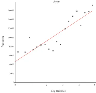
In this analysis, we used a semi-linear variogram, by using the "MVARIOGRAM" in GENSTAT©. Table 1 shows DQH[DPSOHRIWKHHVWLPDWHRIWKHFDOFXODWLRQRIWKHVHPL YDULRJUDPLQDSHULRGRID\HDUEDVHGRQREVHUYDWLRQSRVWV DQGDPD[LPXPVSDFLQJRIPDQGDOHQJWKRIZDV considered when calculating the semi-variogram, homogene-ity in all directions. Where N is the number of observations, h is the length and V is the estimated variance of the
Table 1. Estimations of computing the semi-variogram.
N h V
27 6715.9259
54
56
1.135
66 1.363
69 1.623
64
62 2.121 7393.1452
53
61 2.624
3.142
93
3.626
71 15791.6127
73 12657.9932
4.629
25
After this calculation is performed, an adjustment of a linear estimate of the semi-variogram, obtaining an estimate RIWKHSHUFHQWDJHRIYDULDQFHH[SODLQHGE\WKHPRGHOFDQEH VHHQLQWKHOLQHDU¿WRIWKHPRGHOLQ)LJ
16000
14000
12000
10000
8000
6000
4000
2000
0
0 1 2 3 4 5
Log Distance
V
ar
ia
n
ce
Linear
×
× × ×
× ×
×
×
× ×
× × × × × × × ×
×
Figure 1. Adjustment of the linear model to the semi-variogram.
This analysis uses a statistical hypothesis that performs the calculation of the ratio of the variance, showing how
WKHPRGHOH[SODLQVGDWDYDULDQFH7KXVDYDULDQFHRIDERXW ZRXOGEHLQWHUSUHWHGDVUHVXOWLQJIURPDVWURQJOLQHDU relationship, which can be interpreted as absence of spatial or temporal consistency of precipitation.
0RUHRYHU FORVH WR ]HUR ZRXOG EH W\SLFDO RI D low-linear relationship, which could be interpreted as the absence of spatially and temporal uniform precipitation. As the theoretical model has a linear adjustment, it is observed in the calculation of linear regression model that the best adjust-PHQWH[SODLQVPRVWRIWKHYDULDQFHRIWKHVSDWLDORUWHPSRUDO PD[LPXPSUHFLSLWDWLRQV
The method was used to perform a linear adjustment of WKHVHPLYDULRJUDP,QWKLVW\SHRIDQDO\VLVPRUHFRPSOH[ nonlinear models as model "boundedlinear" and Gaussian could be used. However, it was used the linear model, which although simple has good results. This analysis also tried to consider the spatial homogeneity of variance, however this could not be considered, which would bring the calculation of the semi-variogram with estimates of predominant directions. 7KHDQQXDOUHVXOWVRIWKHYDULDQFHH[SODLQHGE\WKHOLQHDU PRGHOIRUHDFK\HDUEHWZHHQDQGDUHFRPSDUHG ZLWK WKH VLJQDO RI (O 1LxR6RXWKHUQ 2VFLOODWLRQ (162 obtained on the website www.cpc.ncep.noaa.gov, with the aim of correlating changes in scale with the spatial and temporal WUHQGVRIWKHPD[LPXPSUHFLSLWDWLRQ
Figure 2 shows the spatial distribution of jobs and Table 2 shows the 52 rain gauge stations of the National Water Agency (ANA) on the state of Rio Grande do Sul.
Latitude (Deg
rees)
-28
-29
-30
-31
-32
-33
-57 -56 -55 -54 -53 -52 -51
Figure 2. Spatial distribution map of rainfall and weather stations
Table 2. Rainfall stations of ANA in Rio Grande do Sul.
Code Locality Latitude Longitude Network
Passo Tainhas ANA
Antonio Prado ANA
Passo do Prata -51.45 ANA
Passo Migliavaca ANA
Prata -51.62 ANA
Encantado -29.23 ANA
Nova Palmira -29.33 -51.19 ANA
Porto Garibaldi ANA
São Vendelino -59.19 -51.37 ANA
Sapucaia do Sul ANA
Guaiba Country Club -51.65 ANA
Quiteria ANA
São Lourenço do Sul -31.37 -51.99 ANA
Bouqueirão ANA
Passo do Mendonça ANA
Santa Clara do Ingai -53.19 ANA
Botucarai -29.72 ANA
Dona Francisca -29.63 -53.35 ANA
Canguçu -31.39 ANA
Granja São Pedro -31.67 ANA
Ponte Cordeiro de Farias -31.57 -52.46 ANA
Pedras Altas -31.74 -53.59 ANA
Pinheiro Machado ANA
Granja Coronel Pedro Osório -52.65 ANA
Granja Cerrito -32.35 -52.54 ANA
Granja Santa Maria -52.56 ANA
Arroio Grande -32.24 ANA
Granja Osório -32.95 -53.12 ANA
Herval ANA
Paim Filho -51.77 ANA
Sananduva -27.95 ANA
Erebango ANA
Linha Cescon ANA
Alto Uruguai -54.13 ANA
Porto Lucena ANA
Carazinho -52.79 ANA
Colonia Xadrez -52.75 ANA
Giruá -54.34 ANA
Conceição -53.97 ANA
Passo Major Zeferino -54.65 ANA
Passo Viola ANA
Garruchos -55.64 ANA
Passo do Sarmento -55.32 ANA
Fazenda S. Cecília de Butui ANA
Itaqui -29.12 -56.56 ANA
Cacequi ANA
Ernesto Alves -29.37 -54.73 ANA
Furnas do Segredo -29.36 ANA
Jaguarí -29.49 -54.69 ANA
Cachoeira Santa Cecília -55.47 ANA
Passo Mariano Pinto -29.31 ANA
RESULTS
7DEOHVKRZVWKHUHVXOWVRIWKHOLQHDU¿WRIWKHYDULRJUDP
models, calculated by presenting their respective percentages
RIYDULDQFHH[SODLQHGE\WKHOLQHDUPRGHO7KHUHVXOWVVKRZ WKHH[LVWHQFHRIVSHFL¿FVSDWLDODQGWHPSRUDOFRKHUHQFHRIWKH PD[LPXPUDLQIDOOLQVRPH\HDUVLQWKHSHULRGEHWZHHQ DQGRQWKHVWDWHRI5LR*UDQGHGR6XO
1RWHWKDWLQWKLVSHULRGWKHUHZHUHIRXU\HDUVZLWKVLJQL¿FDQW
FRKHUHQFHVSDWLDODQGWHPSRUDODQG 7KHVH\HDUVKDGDQH[SODLQHGYDULDQFHZLWKPRUHPHDQLQJIXO
values for intensities and scales of two, three, and four days. Such characteristics show weather systems, which cycles have a tendency of being timescale of the order of one week.
During the formation of a weather system with these features, in the timescale of a week, there is a combination of
Year Number of
Observations Percentage (%)
0D[,B 0D[,B 0D[,B 0D[,B 0D[,B 'LD0B 'LD0B 'LD0B 'LD0B 'LD0B
1971 33 24 75 71 59
1972 52 59 57 57 63 16
1973 42 53 47 57 32 36 32 25
1974 51 55 43 47 46 45 72 56 52 34
1975 35 39 39 43 49 71 26 33 35
1976 51 15 32 32 7 3 33
1977 49 16 19 14 11
52 42 65 74 79 76 67
1979 15 13 33 7
52 4 2
51 14 25 56 15
49 63 67 63 66 26 37
74 53 5 21 43
49 2 23 15
49 57 75 62 69 45 42 45 79
17 49 41 43 7
49 67 79 79 33 3
49 37 41 46 42 3 4 29
52 27 1 22 4 4
46 15 12
1991 42 13 26 33 33 32 19 5 9
1992 47 1
1993 45 2 7 16
1994 46 9 14 1 9
1995 44 27 46 66 62 3
1996 42 5 9 44 33 31 7
1997 32 36 25 61 15 52 46
47 2 12 64 56
1999 45 35 53 15 57 46 11 12 35 17
41 71 56 55 12
Average 26 32 34 36 13 16 21 21 19
SD 4 24 29 26 19 22 23 24 26
GLIIHUHQWW\SHVRIXSULJKWÀRZRU//-ZKLFKVKRZVPD[LPD
and minima patterns of behavior. They, when associated with
WKHYDOXHVRIDFHUWDLQPDJQLWXGHRI//-DQGPD[LPXPSUHFLSL
-tation, are connected to a particular group of weather systems (atmospheric waves, and locking systems MCS), which are part of a cascade structure comprising the variable climate in this respect, when this occurs, these structures can generate possible in-homogeneities, both spatial and temporal precipitations.
$FFRUGLQJWR7DEOHIRU DQGWKHUHLVVSDWLDOFRKHUHQFHLQ WKHPD[LPXPUDLQIDOOEXWWHPSRUDOFRKHUHQFHZDVQRWREVHUYHG
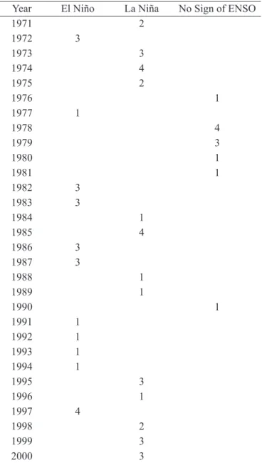
Table 4 shows that El Niño had two predominant situations,
WKHSUHGRPLQDQFHRIVSDWLDOFRKHUHQFH\HDUV¿YH\HDUVDQG \HDUVZLWKRXWVSDWLDODQGWHPSRUDOFRKHUHQFHV¿YH\HDUV,Q
La Niña years, there were three situations, namely: three years with temporal coherence, three years without spatial coher-ence, and temporal and spatial coherence in four years.
7KH\HDUVDQGVKRZHGVSDWLDODQG
temporal coherence and they are also from El Niño, La Niña, and ENSO unsigned.
The spatial coherence years were divided into years with El Niño and La Niña, but the El Niño years have been charac-terized by two predominant situations, with a spatial coherence and the other without spatial and temporal coherences. The weather systems of these periods had a dynamic, in which
WKHUHZDVWKHSUHGRPLQDQFHRIFHUWDLQVSHFL¿FPHWHRURORJLFDO
scales generating spatial coherence.
,Q(O1LxR\HDUVWKH+/-RQ6RXWK$PHULFDH[KLELWJUHDWHU
intensity and persistence than in other phases of ENSO, and, consequently, a greater intensity of LLJ in these periods. The passage of frontal systems, such as short-waves, mesoscale convective and other weather systems with organized
convec-WLYHVWUXFWXUHVWHQGWREHFKDUDFWHUL]HGZLWKPD[LPXPVSDWLDO
coherence, but these weather systems were not the same as the standard for consistency over time, which can be seen in
(O1LxR\HDUVLQ7DEOHVDQG1LFROLQLDQG6DXOR
Liebmann et alDQG6DXORet al
The physical processes that are involved in the generation of precipitations as in MCS have different spatial dimensions, and their formation is associated with different meteorological mechanisms, instabilities forming isolating or forming groups, as in cells Cumulunimbus (Cb) (a few miles) to clusters Cb in a PHVRVFDOHFRQYHFWLYHFRPSOH[0&&ZLWKWHQVWRKXQGUHGV RINLORPHWHUV7KHUHIRUHWKHPD[LPXPUDLQIDOOLQVSDFHPD\
vary from a few to hundreds of kilometers.
This is an important feature of the precipitation, since the generation mechanisms of MCS not always repeat in time,
KDYHGLIIHUHQWVL]HVDQGOLIHF\FOHV7KHH[LVWHQFHRIFOLPDWH
variability in the state of Rio Grande do Sul implies that rain-fall varies in the four seasons, both in intensity and duration
DQGLQDUHDRIFRYHUDJH5DRDQG+DGDGHPRQVWUDWHG WKHH[LVWHQFHRIVLJQL¿FDQWFRUUHODWLRQEHWZHHQSUHFLSLWDWLRQ
in the spring in Rio Grande do Sul and the ENSO signal during the same season or earlier, with the possibility of predicting seasonal rainfall.
7DEOH &RPSDULVRQRIWKHSHUFHQWDJHRIYDULDQFHH[SODLQHGE\ the adjustment of the linear model with the ENSO signal, EHWZHHQWR
Year El Niño La Niña No Sign of ENSO
1971 2
1972 3
1973 3
1974 4
1975 2
1976 1
1977 1
4
1979 3
1
1
3
3
1
4
3
3
1
1
1
1991 1
1992 1
1993 1
1994 1
1995 3
1996 1
1997 4
2
1999 3
3
Data from ENSO. Source: www.cpc.ncep.noaa.gov.
7KH PD[LPXP SUHFLSLWDWLRQ LQ DQG showed no spatial coherence, but showed consistency over time. This fact is interesting because it was La Niña years DQG±DQGPRGHUDWHWRVWURQJWKHFOLPDWLF situation characterizes periods of drought, causing a tendency to decrease frequency and intensity of weather phenomena with different scales on Rio Grande do Sul.
Another important point illustrated in Table 3 shows the situa-tion in which the lack of spatial and temporal coherence, namely, 1993, 1994, 1996, is distributed in all stages of ENOS signal. These periods have not showed characteristics of spatial and temporal coherences, which can result in characterizing the physi-FDOSURFHVVLQWKHJHQHUDWLRQRIPD[LPXPSUHFLSLWDWLRQRI\HDUV ,WVKRZVWKHH[LVWHQFHRIDZLGHYDULHW\RIZHDWKHUDQGVZLWFKLQJ scales of different types of weather structures in space and time.
The different types of weather systems had relations in space, and time variations can occur only at mesoscale, or act in concert with other scales (meso to meso, meso and macro, macro to macro scale), resulting in changes in the characteristics of weather systems, and may intensify them or diminish them in intensity.
The combinations of these structures show a trend of stabil-ity and uniformstabil-ity in growth, development, and persistence of weather systems, hence, an increase of spatial coherence, but these same relationships may or may not have temporal FRKHUHQFH$QH[DPSOHRIWKLVLVZKHQDUHDVDUHIRUPHGE\ divergent instabilities associated with HLJ, they may have irregularities on a spatial region of the order of mesoscale. ,W LV GH¿QHG 0D[,B 0D[,B 0D[,B 0D[,B DQG0D[,BZLWKDPD[LPXPRIRQHGD\RIUDLQDQGWKH PD[LPXPWKDWRFFXUUHGLQWZRWKUHHIRXUDQG¿YHGD\V 7KH'LD0B'LD0B'LD0B'LD0B'LD0BDUH GH¿QHGDVWKHGD\VRIWKH\HDULQZKLFKWKHVHHYHQWVPD[LPXP SUHFLSLWDWLRQRFFXUUHGWKXVH[DPLQHGWKHWHPSRUDOYDULDELOLW\ :KHQWKLVGLYHUJHQFHDVVRFLDWHGZLWK+/-LVLQWHQVL¿HGDQG deepened, generating a wave structure in the atmosphere (tropi-cal cyclones) with a higher spatial and temporal s(tropi-cales, the level of continental scale leads to a dynamic structure and a possibly PRUHKRPRJHQHRXV¿HOGRISUHFLSLWDWLRQ,Q(O1LxR\HDUVWKH HLJ are more intense and persistent and they are associated with //-FRQ¿JXUDWLRQVWKDWKDYHDWHQGHQF\WRVSDWLDOKRPRJHQHLW\
The physical mechanisms of weather systems are strongly baroclinic (turbulent), however, through their relationships between the different meteorological scales involved, their physical properties in space and time change, both intensify and weaken these systems. There is, within this dynamic system, a range of interaction between different synoptic structures, which
is very important in the maintenance and generation of baroclinic DQGFRQYHFWLYHSURFHVVHV7KLVUDQJHLVFKDUDFWHUL]HGE\ÀRZV WKDWRFFXULQWKH3%/ZKLFKLVWKHPD[LPXPWUDQVSRUWLQWKH YHUWLFDOZLQGSUR¿OHRIDVWUXFWXUHZLWK//-7KHUROHRI//-within this turbulent structure is to be a link between the different VSDWLDOVFDOHVRIPHVRPHVRDQGPHVRFRQWLQHQWDOVFDOHV ,QWKLVVLWXDWLRQLQHDFKVSDWLDOVFDOHPD[LPXPUDLQIDOOV are associated. Therefore, in heavy rainfall periods, they are associated with large-scale meteorological vertical develop-ment in the atmosphere, whether as locks, associated with the FRQ¿JXUDWLRQRI+/-ZKHWKHUDVYRUWLFHVFROGDWDOWLWXGHLQ the atmosphere and the years of ENSO (El Niño), with strong LLJ. This structure of continental scale and meso, with strong //-FDQJHQHUDWHPD[LPXPSUHFLSLWDWLRQZLWKUHJXODUGLVWUL-bution in space and time, the size of the spatial and temporal scale involved, as the year of 1997.
In other situations, the LLJ may be weaker and predomi-nant in the order and mesoscale, which can generate and maintain structures and baroclinic instabilities that can cause irregular or regular precipitations in space and time. In this FRQWH[WZLWKLQWKLVG\QDPLFVWUXFWXUHGHVFULEHGWKHÀRZRU LLJ always occurs, independent of whether there is spatial homogeneity or temporal variability of rainfall.
Therefore, the same weather scale may act differently in WKHJHQHUDWLRQRIPD[LPXPUDLQIDOOIHDWXULQJDYHU\FRPSOH[ structure that comprises a set of dynamic weather systems, DQG ZKLFK WRJHWKHU IRUP WKH ¿HOG RI SUHFLSLWDWLRQ DQG LV LQÀXHQFHGE\ORFDOIDFWRUVZLWKUHJLRQDODQGODUJHVFDOHV
CONCLUSIONS
REFERENCES
Abdoulaev, S. et al ³6LVWHPDV GH 0HVRHVFDOD GH Precipitações no Rio Grande do Sul. Parte 2: Tempestades em Sistemas não lineares de convecção severa”, Revista
%UDVLOHLUDGH0HWHRURORJLD9RO1RSS
Abdoulaev, S. et al³,QWHUQDO6WUXFWXUHRI1RQ/LQH Mesoscale Convective System in Southern Brazil”, In: Congresso Brasileiro De Meteorologia, Campos do Jordão,
$QDLVYSS
'H %DUURV 6 6 2\DPD 0 ' ³6LVWHPDV 0HWHR
-rológicos Associados à Ocorrência de Precipitação no Centro de Lançamento de Alcântara”, Revista Brasileira de Meteoro-logia, Vol. 25, No. 3, pp. 333-344.
%HUEHU\(+&ROOLQL($³6SULQJWLPHSUHFLSLWDWLRQ DQGZDWHUYDSRUÀX[FRQYHUJHQFHRYHUVRXWKHDVWHUQ6RXWK $PHULFD´0RQWKO\:HDWKHU5HYLHZ9ROSS
&RUUrD&6³(VWXGRHVWDWtVWLFRGDRFRUUrQFLDGHMDWRVQR SHU¿OYHUWLFDOGRYHQWRQDEDL[DDWPRVIHUDHDVXDUHODomRFRP
eventos de intensa precipitação pluvial no Rio Grande do Sul” (In Portuguese), PhD Thesis, Instituto de Pesquisas Hidráulicas, Universidade Federal do Rio Grande do Sul, Porto Alegre.
&KHQ *7- <X && ³6WXG\ RI ORZOHYHO MHW DQG H[WUHPHO\KHDY\UDLQIDOORYHUQRUWKHUQ7DLZDQLQWKH0HL<X VHDVRQ´0RQWKO\:HDWKHU5HYLHZ9RO1RSS
Chen, C. et al ³$ 6WXG\ RI D 0RXQWDLQJHQHUDWHG Precipitation System in Northern Taiwan during TAMEX IOP
´0RQWKO\:HDWKHU5HYLHZ9RO1RSS
+HOIDQG + 0 6FKXEHUW 6 ' ³&OLPDWRORJ\ RI
simulated great plains low-level jet and its contribuition to the continental moisture budget of the United States”, Journal of
&OLPDWH9RO1RSS
Higgins, R. W. et al³,QÀXHQFHRIWKHJUHDWSODLQV low-level jet on summertime precipitation and moisture transport over the central United States”, Journal of Climate,
9ROSS
+XLMEUHJWV&-³5HJLRQDOL]HGYDULDEOHVDQGTXDQWLWD
-tive analysis of spatial data”, In: Davis, J. C., McCullagh, M. J. (ed.), Display and analysis of spatial data, New York, John
:LOH\SS
/DFNPDQQ * 0 ³&ROGIURQWDO SRWHQWLDO YRUWLFLW\
PD[LPDWKHORZOHYHOMHWDQGPRLVWXUHWUDQVSRUWLQH[WUDWURSL
-FDOF\FORQHV´0RQWKO\:HDWKHU5HYLHZ9ROSS
Liebmann, B. et al³6XEVHDVRQDO9DULDWLRQVRI5DLQIDOO in South America in the vicinity of the Low-level Jet East of the Andes and Comparison to those in the South Atlantic
Conver-JHQFH=RQH´-RXUQDORI&OLPDWH9ROSS
0DGGR[5$'RVZHOO,,,&$³$QH[DPLQDWLRQRIMHW VWUHDPFRQ¿JXUDWLRQVPEYRUWLFLW\DGYHFWLRQDQGORZOHYHO WKHUPDODGYHFWLRQSDWWHUQVGXULQJH[WHQGHGSHULRGVRILQWHQVH FRQYHFWLRQ´0RQWKO\:HDWKHU5HYLHZ9ROSS
1LFROLQL0DQG6DXOR$&³(WDFKDUDFWHUL]DWLRQRI WKHZDUPVHDVRQ&KDFRMHWFDVHV´3UHSULQWVRI
the 6th International Conference on Southern Hemisphere
0HWHRURORJ\DQG2FHDQRJUDSK\&KLOHSS
5DR9%+DGD.³&KDUDFWHULVWLFVRI5DLQIDOORYHU %UD]LO±DQQXDOYDULDWLRQVDQGFRQQHFWLRQVZLWKWKHVRXWKHUQ
oscillation”, Theoretical and Applied Climatology, Vol. 42,
1RSS
Saulo, A. C. et al³6\QHUJLVPEHWZHHQWKH/RZOHYHO
-HWDQG2UJDQL]HG&RQYHFWLRQDWLWVH[LW5HJLRQ´0RQWKO\ :HDWKHU5HYLHZ9ROSS
8FFHOOLQL / : -RKQVRQ ' 5 ³7KH FRXSOLQJ RI
upper and lower tropospheric jet streaks and implications for the development of severe convective systems”, Monthly
:HDWKHU5HYLHZ9RO1RSS