INTRODUCTION
In the last four decades, a great number of numerical methods have been developed for computing solutions to optimal control problems. These methods are divided into two main classes: indirect and direct. The indirect ones involve the solution of a nonlinear two-point boundary value problem obtained from a set of necessary conditions for a local extre-mum of the objective function, provided by the Pontryagin’s Maximum Principle (Pontryagin et al., 1962) or the calculus of variations (Bliss, 1946; Hestenes, 1966). For instance, the quasilinearization method, also known as generalized Newton-Raphson method (McGill and Kenneth, 1964), and the shooting one (Sage and White, 1977) belong to this class of numerical methods. On the other hand, the direct methods use only equations of motion and terminal conditions and they attempt to minimize the objective function through an itera-WLYHGHVFHQWSURFHGXUH7KHGLUHFWDSSURDFKZDV¿UVWSURSRVHG by Kelley (1960) and is referred to as the gradient method.
Other direct methods are the steepest descent method (Bryson and Denham, 1962) and the ones based upon the second variation theory (Bullock and Franklin, 1967; Long-muir and Bohn, 1969; Bryson and Ho, 1975). These direct methods use the calculus of variations, but there is another class of direct methods that transform optimal control prob-lems into nonlinear programming ones, such as the direct transcription or collocation method (Betts, 1993; 1994) and the direct methods based on differential inclusion concepts (Seywald, 1994; Coverstone-Carroll and Williams, 1994).
In this paper, the steepest descent method and the direct method based upon the second variation theory, which will be referred to as second variation method, are discussed, considering different algorithms in comparison to the original ones proposed by Bryson and Denham (1962) and Longmuir and Bohn (1969). The steepest descent method was developed IRUD0D\HUSUREOHPRIRSWLPDOFRQWUROZLWKIUHH¿QDOVWDWH DQG¿[HGWHUPLQDOWLPHV7HUPLQDOFRQVWUDLQWVRQVWDWHYDUL-ables were considered through the penalty function method (Hestenes, 1969; O’Doherty and Pierson, 1974). A procedure to adjust the step size in control space is proposed to improve the convergence rate and avoid the divergence of the method
A Review of Gradient Algorithms for Numerical Computation
of Optimal Trajectories
Wander Almodovar Golfetto1,*, Sandro da Silva Fernandes²
1Departamento de Ciência e Tecnologia Aeroespacial – São José dos Campos/SP – Brazil 2Instituto Tecnológico de Aeronáutica – São José dos Campos/SP – Brazil
Abstract: In this paper, two classic direct methods for numerical computation of optimal trajectories were revisited: the steepest descent method and the direct one based upon the second variation theory. The steepest descent method was developed for a 0ayer problem of optimal control, with free ¿nal state and ¿[ed terminal times. Terminal constraints on the state variables were considered through the penalty function method. The second method was based upon the theory of second variation and it involves the closed-loop solutions of a linear quadratic optimal control problem. The algorithm was developed for a Bolza problem of optimal control, with ¿[ed terminal times and constrained initial and ¿nal states. 3roblems with free ¿nal time are also considered by using a transformation approach. $n algorithm that combines the main characteristics of these methods was also presented. The methods were applied for solving two classic optimization problems – Brachistochrone and Zermelo – and their main advantages and disadvantages were discussed. Finally, the optimal space trajectories transference between coplanar circular orbits for different times of Àight was calculated, using the proposed algorithm.
Keywords: Optimization of trajectories, Numerical methods, Steepest descent method, Second-order gradient method.
Received: 26/01/12 Accepted: 18/03/12
*author for correspondence: [email protected]
as the optimal solution is approached. On the other hand, the second order gradient method involves the determination of closed-loop solutions of a linear quadratic optimal control problem using the Riccati transformation. The algorithm was developed for a Bolza problem of optimal control, with ¿[HGWHUPLQDOWLPHVDQGFRQVWUDLQHGLQLWLDODQG¿QDOVWDWHV$ VOLJKWPRGL¿FDWLRQRIWKHDOJRULWKPZDVPDGHWRVDWLVI\WKH Legendre condition and avoid the divergence of the method (Bullock and Franklin, 1967). In both methods, problems with IUHH¿QDOWLPHDUHWUHDWHGE\XVLQJDWUDQVIRUPDWLRQDSSURDFK that introduces a new independent variable and an additional control one, and transforms a time-free problem in a new WLPH¿[HGRQH+XVVX4XLQWDQDDQG'DYLVRQ The methods are applied in solving two classic optimiza-tion problems – Brachistochrone and Zermelo problems –, and their main advantages and disadvantages are discussed. Finally, an algorithm that combines the main positive charac-teristics of these methods was presented and applied in space trajectories optimization for transference between coplanar circular orbits.
STEEPEST DESCENT METHOD
The steepest descent method is an iterative direct method widely used for computing a m-vector of control variables
f
t
t
t
t
u
(
),
0d
d
, which minimizes a scalar performance index in an optimization problem (Kelley, 1960; Bryson and Denham, 1962; McIntyre, 1968; McDermott and Fowler, 1977).$ VLPSOL¿HG YHUVLRQ RI WKH VWHHSHVW GHVFHQW PHWKRG was here presented for a Mayer problem of optimal control ZLWKIUHH¿QDOVWDWHDQG¿[HGWHUPLQDOWLPHV3UREOHPVZLWK FRQVWUDLQWVRQWKHVWDWHYDULDEOHVDWWKH¿QDO¿[HGWLPHZHUH treated by using the penalty function method (Hestenes, 2¶'RKHUW\DQG3LHUVRQDQGWKRVHZLWKIUHH¿QDO time were treated by using a transformation approach, which introduces new independent and additional control variables +XVVX4XLQWDQDDQG'DYLVRQ'HWDLOVRIWKLV WHFKQLTXHDUHIXUWKHUGHVFULEHG7KXVWKLVVLPSOL¿HGYHUVLRQ has two main features: the algorithm is very simple, requiring a single numerical integration of the adjoint equations at each step, and some of the typical divergence problems described by McDermott and Fowler (1977) are circumvented.
Consider the system of differential equations (Eq. 1):
n
i
u
x
f
dt
dx
i i
,...,
1
),
,
(
,
(1)where:
[ is a n-vector of state variables; u is a m-vector of control variables; f(.):Rn uRm oRn, fi (.) and wfi wxj, i and j = 1,...,nDUHGH¿QHGDQGFRQWLQXRXVRQRn × Rm. It is assumed that there are no constraints on the state or control variables.
The problem consists in determining the control u*(t) that transfers the system (Eq. 1) from the initial conditions (Eq. 2):
[(t0) = [0, (2)
WRWKH¿QDOFRQGLWLRQVDWtf (Eq. 3):
[(tf) = free, (3)
and minimizes the performance index (Eq. 4):
J[u] = g([(tf)), (4)
with g R: noR
and wg wxi, i =1,...,n, continuous on R n
. For completeness, a brief description of the steepest descent method is presented. The development of the algorithm was based on the classic calculus of variations (Bliss, 1946; Hestenes, 1966; Gelfand and Fomin, 1963; Elsgolts, 1977). Introducing the n-vector Ȝ of Lagrangian multipliers – adjoint variables –, the augmented performance index is formed as Eq. 5:
>
H x@
dt tx g J
f t
t
T
f
³
0
)) (
( O , (5)
where, H is the Hamiltonian function (Eq. 6),
)
,
(
)
,
,
(
x
u
f
x
u
H
O
O
T.
(6)Let u0(t), t
0 t tf be an arbitrary starting approximation of the control u*(t), t
0 t tf and [ 0(t), t
0 t tfthe correspond-ing trajectory, obtained by integratcorrespond-ing the system (Eq.1). Let
f
t t t t u t u t
u1( ) 0()
G
(), 0 d dbe the second iterate such that J[u1@ J[u0]. It is assumed that the control variation
f
t t t t
u( ), 0 d d
G
is small, in order that the linearity assump-tions are valid, and they satisfy the constraint as in Eq. 7:2
0
)
(
)
(
)
(
W
u
d
K
u
f tt T
³
G
W
W
G
W
W
,
(7)the step size in control space. Both W(IJ) and K must be chosen by the user of the algorithm.
The control variation įu(t),t0 t tfcauses perturbations in the state vector so that the corresponding trajectory to the control u1(t),t
0 t tf , can be expressed as [
1(t) [0(t)į[(t). Accordingly, the change in J¯, which is assumed to be
GLIIHUHQWLDEOHWR¿UVWRUGHULQWKHSHUWXUEDWLRQVLVJLYHQE\
Eq. 8 (McIntyre, 1968):
>
g t@
x t>
>
H@
x H u Jf
f
t
t
u T x f
f T
x
³
0 ) ( )
( G O G G
O
G , (8)
since į[(t0) = 0, taking the n-vector Ȝ of the Lagrangian
PXOWLSOLHUV ± DGMRLQW YDULDEOHV ± VXFK WKDW LW VDWLV¿HV WKH
system of differential equations (Eq. 9):
d
dt
H
xT
O
,
(9)and the boundary conditions (Eq. 10)
T x
f
g
ft
)
(
O
,
(10)Equation 8 reduces to Eq. 11:
³
ft
t
u
udt
H
J
0
G
G
.
(11)(TXDWLRQVDQGGH¿QHDQLVRSHULPHWULFSUREOHPRIWKH
calculus of variations, solution of which is given by Eqs. 12 and 13 (Gelfand and Fomin, 1963; Elsgolts, 1977):
T u
H
W
u
12
1
Q
G
,
(12)2 / 1
1
0
2 1
°¿ ° ¾ ½ °¯
° ®
³
ft
t
T u
uW H dt
H K
Q
, (13)where
Q
is the Lagrangian Multiplier corresponding to the constraint (Eq. 7).Thus, from Eqs. 11 to 13, it follows Eq. 14:
2 / 1
1
0
°¿
°
¾
½
°¯
°
®
³
ft
t
T u u
W
H
dt
H
K
J
J
G
G
,
(14)and the new value of the performance index will be smaller than the previous ones.
The step-by-step computing procedure to be used in the steepest descent method is summarized as:
,QWHJUDWHWKHGLIIHUHQWLDOHTXDWLRQV(TIURPWKHLQLWLDO
point [0 at t0WRDQXQVSHFL¿HG¿QDOSRLQW[(tf) at tf , with the nominal control u0(t), t
0 t tf ;
,QWHJUDWHWKHDGMRLQWGLIIHUHQWLDOHTXDWLRQV(TIURPtf to t0 , with the terminal conditions (Eq. 10);
&RPSXWHWKH/DJUDQJLDQPXOWLSOLHU
Q
from Eq. 13; &RPSXWHWKHFRQWUROµFRUUHFWLRQ¶
G
u(t),t0 dtdtf from Eq. 12; 2EWDLQDQHZQRPLQDOFRQWUROE\XVLQJu1(t) u0(t)Gu(t),
and repeat the process until the integral
³
f t
t
T u
u
W
H
dt
H
0
1
WHQGVWR]HURRURWKHUFRQYHUJHQFHFULWHULRQLVVDWLV¿HG
It should be noted that as the nominal control un(t)
approaches the optimal one u*(t), the integral
³
f t
t
T u
u
W
H
dt
H
0
1
approaches zero and the Lagrangian multiplier
Q
tends to]HURWKXVWKHFRQWUROµFRUUHFWLRQ¶įu(t), obtained from Eq. 12, can become too large and the process diverges. In order to avoid this drawback, the step size in control space K must
EHUHGH¿QHG7KHIROORZLQJKHXULVWLFDSSURDFKLVSURSRVHG
suppose that Km is the step size in control space at the m-th
iterate, if
³
f t
t
T u
u
W
H
dt
H
0
1
< L , where L is a critical value
for this integral, then KLVUHGH¿QHGDVKm1
E
Km, with0 < ȕ< 1 as a reduction factor. L and ȕ must be chosen by the user of the algorithm. Numerical experiments have shown that this approach provides good results.
SECOND VARIATION METHOD
The direct method based upon the second variation is also an iterative method used for computing a m-vector of control variables u(t),t0dtdtf, which minimizes a scalar performance index in an optimization problem (Bullock and Franklin, 1967; Longmuir and Bohn, 1969; Bryson and Ho, 1975; Imae, 1998). In the present work, this method will be simply referred to as a second variation method.
The second variation method is developed for a Bolza
SUREOHPRIRSWLPDOFRQWUROZLWKFRQVWUDLQHG¿QDOVWDWHDQG ¿[HGWHUPLQDOWLPHV7KHJHQHUDOL]HG5LFFDWLWUDQVIRUPDWLRQDV
with the accessory minimization problem obtained from the second variation of the augmented performance index of the original optimization problem. Therefore, the algorithm here presented is different from the one described by Bullock and Franklin (1967), which was developed for a Mayer problem and involves a different set of transformation matrices for solving the linear two-point boundary value problem associated with the accessory minimization problem. The present algorithm is also different from the one proposed by Bryson and Ho (1975), since it does not include the stopping condition for time-free problems, which are treated by a transformation approach as mentioned. However, the algorithm is closely based on the approach for second variation methods described by Longmuir DQG%RKQDQGLQFOXGHVDQLPSRUWDQWPRGL¿FDWLRQDGRSW -ed by Bullock and Franklin (1967) in their algorithm in order to assure the convergence and to satisfy Legendre’s condition.
For completeness, a brief description of the development of the second variation method is presented. Consider the system of differential equations (Eq. 15):
n
i
u
x
f
dt
dx
ii
(
,
),
1
,...,
,
(15)where, [ is a n-vector of state variables and u is a m-vector of control variables, f(.):RnuRm oRn, fi(.) e wfi wxj, i and j =1,...,nDUHGH¿QHGDQGFRQWLQXRXVRQRn×Rm. It is assumed that there are no constraints on the state or control variables.
The problem consists in determining the control u*(t), which
transfers the system (Eq. 15) from the initial conditions (Eq. 16):
[(t0) = [0, (16)
WRWKH¿QDOFRQGLWLRQVDWtf (Eq. 17):
ȥ([(tf )) = 0, (17)
and minimizes the performance index (Eq. 18):
)
,
(
))
(
(
]
[
0dt
u
x
F
t
x
g
u
J
f t tf
³
,
(18)with g: Rnĺ R and g[i, i =1,...,n, continuous on Rn. F(.) and F[i , i =1,...,n DUH DOVR GH¿QHG DQG FRQWLQXRXV RQ Rn×Rm, and ȥ:Rn ĺ Rq, q<n, ȥ
i (.) and ȥi [j, i=1,...,q, and j=1,...,nDUHGH¿QHGDQGFRQWLQXRXVRQRn. Furthermore, it is
assumed that the matrix »¼ º «¬ ª w w x
\ has maximum rank.
The second variation method is an extension of the steepest descent one already presented and it is also based on the classic calculus of variations. The main difference is the inclusion of the second-order terms in the expansion of the augmented performance index about a nominal solution. By virtue of this fact, the method is also known as second-order gradient method (Bryson and Ho, 1975).
Introducing the n-vector Ȝ of Lagrangian multipliers – adjoint variables – and the q-vector ȝ of Lagrangian multipliers, the augmented performance index is formed by Eq. 19:
>
@
³
f t t T f Tf xt H xdt
t x g J 0 )) ( ( )) (
( P \ O . (19)
Here, the Hamiltonian function H is defined as H([,Ȝ,u) = -F([,u) + ȜTƒ[,u.
In order to derive the algorithm of the second variation method, one proceeds as in the steepest descent method. Let u0(t), t
0ttƒ be an arbitrary starting approximation of the control u*(t), t
0ttƒ ; [0(t), t
0ttƒ , the corresponding trajectory, obtained by integrating the system (Eq. 1) and ȝ0 be an arbitrary starting approximation of the Lagrange multiplier ȝ. And, u1(t) = u0(t) + įu(t), t
0ttƒ, be the second iterate such that J[u1@J[u0]. The control variation įu(t), t0ttƒ causes perturbations in the state vector [(t), as well in the adjoint vector Ȝ(t) and in the Lagrange multiplier ȝ, so that the nominal values of [(t), Ȝ(t) and ȝ, corresponding to the control u1(t), t
0ttƒ can be expressed as Eq. 20:
[1(t) = [0(t) + į[(t), t 0ttƒ Ȝ1
(t) = Ȝ0(t) + įȜ(t), t 0ttƒ
ȝ1 ȝ0įȝ. (20)
It is assumed that the perturbations į[,įȜ, įu and įȝ are small. Therefore, the change in ¯J, which is assumed to be twice differentiable, to second order in the perturbations, is given by Eq. 21 (Longmuir and Bohn, 1969):
Considering that the state equations (Eq. 15) is as in Eq. 22:
T
H
dt
dx
O
,
(22)with the initial conditions [(t0)=[0LVVDWLV¿HGDVZHOODVWKH
adjoint equations (Eq. 23)
d
dt Hx
T
O , (23)
with the boundary conditions (Eq. 24)
Ȝ(tf) = -(gx + ȝTȥ
[)T; (24)
and taking Eq. 25
ȥxįx(tf) = -ȥ([(tf)), (25)
Eq. 21 reduces to 26:
, 2 1 2 1 ) ( ) ( 2 1 0 dt x u H u u H u H x H x x H x u H t x g t x J T uu T u T t t xu T x T xx T u f xx T xx T f f ¸ ¹ · ¨ © §³
G GO G G G GO G G GO G G G G G \ P G ' O O (26)since į[(t0) = 0. Notice that į[(tVDWLV¿HVWKHOLQHDUSHUWXUEDWLRQ
equation (Eq. 27):
į[ʞ = HȜ[į[ HȜuįu. (27)
The change in the performance index, including the second order terms, can be written as Eq. 28:
, 2 1 2 1 ) ( ) ( 2 1 0 dt u H u u H x x H x u H t x t x J f t t uu T xu T xx T u f xx T f
³
¸ ¹ · ¨ © § G G G G G G G G ) G ' (28)Where (Eq. 29):
ĭ[[ = g[[ + ȝTȥ
[[. (29)
7KH SUREOHP RI GHWHUPLQLQJ įu(t LV WKHQ GH¿QHG E\
the following new problem of optimal control, known as accessory problem (Bullock and Franklin, 1967): determine
įu(t), t0ttƒ to minimize the performance index ǻ ¯JGH¿QHG
by Eq. 28, subject to Eqs. 30 to 32:
į[ʞ = HȜ[į[ HȜuįu, (30)
į[(t0)= 0, (31)
ȥxįx(tf) = -ȥ([(tf)). (32)
Following the Pontryagin’s Maximum Principle
(Pontryagin et al., 1962), the n-vector p of adjoint variables
is introduced and the Hamiltonian function H˾(į[, p, įu) is
formed by using Eq. 30:
H x H up u H u u H x x H x u H u p x H u x T uu T xu T xx T u G G G G G G G G G G G O O ¸ ¹ · ¨ © § 2 1 2 1 ) , , ( ~ . (33)
The optimal control įu*(t) (Eq. 34) must be chosen to
maximize the Hamiltonian H˾(Eq. 33):
]. [ 1 p H x H H H
u uu uT uxG uO
G (34)
The adjoint vector p(t) must satisfy the differential Eq. 35:
pʞ=-H[Ȝp - (H[[į[ H[uįu), (35)
with the boundary conditions (Eq. 36):
p(tf) = -ĭ[[į[(tf)-ȥT
[ı, (36)
where ı is the Lagrangian multiplier corresponding to the
constraint (Eq. 32). Note that Equations 35 and 36 are the linear perturbation ones corresponding to Eqs. 23 and 24,
respectively; thus, p(t)=įȜ(t) and ı = įȝ.
Substituting įȝ*(t) into Eqs. 30 and 35, the following
two-point boundary value problem is obtained (Eq. 37):
į[ʞ = $į[ BįȜ'
įȜʞ = Cį[ - $TįȜ(, (37)
where the matrices $, B, C, ', ( are given by Eq. 38:
$ = HȜ[ - HȜuHuu-1Hu[
B = -HȜ[Huu-1HuȜ
C = H[uHuu-1Hu[ - H[[ (38)
' = - HȜuHuu-1Hu
with the boundary conditions (Eqs. 39 to 41):
į[(t0) = 0, (39)
ȥ[į[(tf) = -Nȥ([(tf)), (40)
įȜ(tf) = -ĭ[[į[(tf) - ȥT[įȝ, (41)
with 0 < k < 1.
Equation 40 means that on each step, “partial corrections” are obtained. The parameter k must be chosen by the user of the algorithm. Numerical experiments show that this parameter can be used to avoid the method diverges.
The solution of the two-point boundary value problem DERYH GH¿QHG LV REWDLQHG WKURXJK D EDFNZDUGVZHHS method, which uses the generalized Riccati transformation (Longmuir e Bohn, 1969; Bryson and Ho, 1975), as in Eqs. 42 and 43:
įȜ(t) = R(t)į[(t) + L(t)įȝ + s(t), (42)
0 = LT(t)į[(t) + Q(t)įȝ + r(t), (43)
where:
R is a n × n symmetric matrix,
L is a n × q matrix,
Q is a q × q symmetry matrix,
s is a n × 1 matrix, and r is a q × 1 matrix.
In order that Eqs. 42 and 43 be consistent with Eqs. 37 WR WKH 5LFFDWL FRHI¿FLHQWV PXVW VDWLVI\ WKH IROORZLQJ differential equations (44 to 48):
-Rʞ = R$ + $TR + RBR - C, (44)
-Lʞ = ($T + RB)L, (45)
-Qʞ = LTBL, (46)
-sʞ= ($T +RB)s + R' - (, (47)
-rʞ= LT(' + Bs), (48)
with the boundary conditions (49 to 53):
R(tf )=-ĭ[[, (49)
L(tf )=-ȥ[T, (50)
Q(tf )=0, (51)
s(tf )=0, (52)
r(tf )=-k ȥ. (53)
The step-by-step computing procedure to be used in the second variation (or second order gradient) method is summarized as follows:
,QWHJUDWHWKHGLIIHUHQWLDOHTXDWLRQVIURPWKHLQLWLDO point [0 at t0WRDQXQVSHFL¿HG¿QDOSRLQW[(tf) at tf, with the starting nominal control u0(t),t
0 t tf ; &KRRVHDVWDUWLQJ/DJUDQJHPXOWLSOLHUȝ0;
,QWHJUDWHWKHDGMRLQWGLIIHUHQWLDOHTXDWLRQVIURPtf to
t0, with the boundary conditions (24);
&RPSXWHWKHSDUWLDOGHULYDWLYHVRIWKH+DPLOWRQLDQIXQF-tion H - Hu, Huu, H[u, H[Ȝ, H[[ and HȜu ;
,QWHJUDWH(TVWREDFNZDUGIURPtf to t0, with the ERXQGDU\FRQGLWLRQVGH¿QHGE\(TVWR&RPSXWH
R(t), L(t), Q(t), s(t) and r(t); &RPSXWHįȝ=-Q(t0)-1[LT(t
0)į[(t0)+r(t0)];
,QWHJUDWH WKH OLQHDU SHUWXUEDWLRQ HTXDWLRQ
į[ǜ=($+BR)į[+BLįȝ+Bs+', obtained from Eqs. 37 and 42; &RPSXWHįȜ(t) using Eq. 42;
&RPSXWHįu* using Eq. 34;
&RPSXWHWKHQHZFRQWUROu1(t)=u0(t)+įu(t), t
0 t tf, and the Lagrange multiplier ȝ1=ȝ0+įȝ;
7HVWWKHFRQYHUJHQFH5HSHDWWKHSURFHVVXQWLOLWFRQYHUJHV
It should be noted that the algorithm of the second variation method diverges if the Legendre condition Huu < 0, computed for the nominal solution over the whole time interval t0 t tf LVQRWVDWLV¿HG+RZHYHUE\DGGLQJDWHUP
³
tf tTW udt
u u
0 2 2
2 1
2 1
G
G
G
, which further constraints thecontrol effort, the resulting functional ǻJĀ
THE COMBINED ALGORITHM
As discussed in the book by Bryson and Ho (1975), the main characteristic of the steepest descent method is the great
LPSURYHPHQWVLQWKH¿UVWIHZLWHUDWLRQVEXWLWKDVSRRUFRQYHU -gence as the optimal solution is approached. On the other hand, the second variation method presents excellent convergence characteristics as the optimal solution is approached, but it
UHTXLUHVWKHQRPLQDOVROXWLRQWREHµFRQYH[¶$OWKRXJKWKH PRGL¿FDWLRQLQWURGXFHGLQWKHDOJRULWKPSURYLGHVWKHUHTXLUHG
convexity conditions, numerical experiments have shown that the accuracy of the solution is very sensitive to the choice of matrix W2LIWKH¿UVWDSSUR[LPDWLRQRIWKHFRQWUROLVSRRU
Considering these remarks, an algorithm that combines the best characteristics of each method is implemented: at the
¿UVWVWHSWKHVWHHSHVWGHVFHQWPHWKRGLVDSSOLHGWRLPSURYHWKH
nominal solution to a point where it is convex; then, at the second one, the second variation method is applied, using the value of u
REWDLQHGDVWKHVROXWLRQRIWKH¿UVWDOJRULWKPDVWKHLQLWLDOJXHVV
of the second one. The point where the algorithm commutes
IURPWKHVWHHSHVWGHVFHQWWRWKHVHFRQGRUGHUPHWKRGLVGH¿QHG
by the user and is based on the value desired for the integral:
HuW-1HuTdt.The resulting algorithm will be simply referred to as the combined algorithm and its implementation is a combination of the step-by-step computing procedure. As it will be later presented,
WKHFRPELQHGDOJRULWKPEDVHGRQWKHVLPSOL¿HGYHUVLRQVRIWKH
steepest descent and second variation methods described in the preceding sections provides good results, which have motivated its application to the analysis of optimal low-thrust limited-power transfers between coplanar circular orbits.
SIMPLE NUMERICAL EXAMPLES
In order to clarify some of the algorithms aspects of the methods described, two classical examples were considered: the Zermelo and the Brachistochrone problems.
Zermelo problem
It is a classical minimum-time navigation problem (Leitmann, 1981). Consider a boat moving with velocity v of constant magnitude v =1 relative to a stream of constant velocity s. The problem consists in determining the steering
program that transfers the boat from a given initial position to a given terminal position in minimum time. The statement of the optimization problem is as follows: determine the control ș(t) that transfers the system described by differential equations (54):
s dt
dx
T
cos
1 2 sinT
dt dx
1
3 dt dx
, (54)
from the initial (55)
[i(t0)=[i
0 ,i = 1,2,3, (55)
WRWKH¿QDOFRQGLWLRQV
[1(tf )= [1
f [ 2(tf )= [2
f, (56)
and minimizes the performance index (57)
J= [3(tf ). (57)
In order to solve this time-free problem by means of the algo-rithms of the steepest descent and the second variation methods, a transformation approach must be used. This time-free problem
ZLOOEHWUDQVIRUPHGLQDQHZWLPH¿[HGSUREOHPWKURXJKDVLPSOH GHYLFH+XVVX4XLQWDQDDQG'DYLVRQ
,QWURGXFLQJ QHZ LQGHSHQGHQW IJ IJ[0,1] and auxiliary control variables Į through the Eq. 58
t = ĮIJ, (58)
WKHWLPHIUHHSUREOHPGH¿QHGE\(TVWRLVFRQYHUWHGWR DWLPH¿[HGSUREOHPZLWKVWDWHHTXDWLRQVJLYHQE\
sd dx
T D W cos
1
T D W sin
2
d dx
D W
d dx
3
(59)
In order to apply the algorithm of the steepest descent method
GHULYHGIRUD0D\HUSUREOHPZLWKIUHH¿QDOVWDWHWKHSHQDOW\
function method (Hestenes, 1969; O’Doherty and Pierson,
PXVWEHXVHG7KHQHZWLPH¿[HGSUREOHPLVWKHQGH¿QHG
by the state equations (59), the initial conditions (55), and a new performance index obtained from Eqs. 56 and 57:
>
2@
2 2 2 2 1 1 1
3(1) (1) (1)
f
f k x x
x x k x
J
,
(60)where k1,k2 >> 1 must be chosen by the user of the algorithm. In the penalty function method as described by O’Doherty and Pierson (1974), the penalty constants k1 and k2 are
value for these constants as adopted by Lasdon et al. (1967) in the conjugate gradient method.
Both methods use the partial derivatives of the Hamiltonian function H, which is given by H=Į[Ȝ1(cosș+s)+Ȝ2sinș+Ȝ3].
As an example, consider s=WKHLQLWLDODQG¿QDO
SRLQW7KHH[DFWVROXWLRQZLWKVHYHQVLJQL¿FDQW¿JXUHV
of this problem is tf=7KH¿UVWDSSUR[LPDWLRQRIWKH
control variables is chosen as Eqs. 61 and 62 for both algorithms:
ș(IJ) = 0.5,IJ[0,1], (61)
Į(IJ) = 2.0,IJ[0,1], (62)
The numerical results are shown in Table 1 and Figs. 1 to 3. In both cases, the convergence criterion is given by |I3n+1-I3n| < 1.25×10⁻⁷.
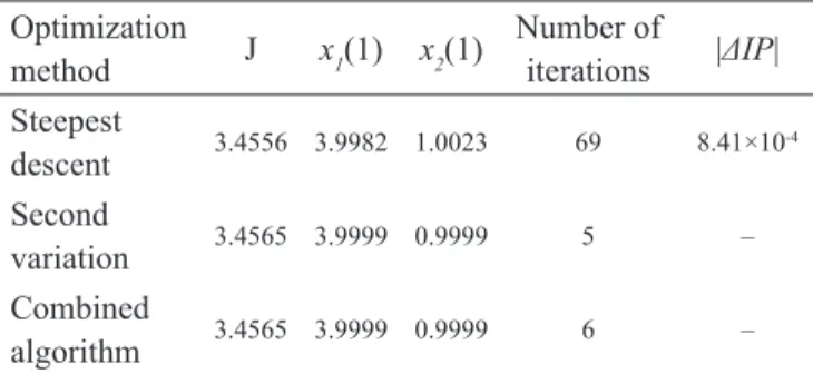
Table 1. Numerical results for Zermelo problem.
Optimization
method J [1(1) [2(1)
Number of
iterations |ǻI3|
Steepest
descent 3.4556 3.9982 1.0023 69 8.41×10
-4
Second
variation 3.4565 3.9999 0.9999 5 –
Combined
algorithm 3.4565 3.9999 0.9999 6 –
For the steepest descent method, the numerical results are obtained with the following set of parameters: weights of the
penalty function, k1=k2=500; reduction factor for the step size in
control space, ȕ=0.50; initial step size in control space K0=0.05;
critical value of the integral
³
f t
t
T u uW H dt
H
0
1
, L=1000. For the
second variation method, the numerical results are presented with the following set of parameters: reduction factor for partial
FRUUHFWLRQVRIWKHWHUPLQDOFRQVWUDLQWGH¿QHGLQ(Tk=1.0;
reduction factor for įuDQGįȝ corrections (0< İ 1), İ=1.0;
elements of the diagonal matrix W2, Wii,2= -2000. For simplicity,
W2 has been chosen as a diagonal matrix. For this set of
param-eters, the second variation method requires less iterations than the steepest descent method and the accuracy of the solution is much better. The last column provides a difference between the value of the performance index obtained through the algorithms and the exact solution. In Fig 1, the rates of convergence for steepest descent and second variation methods are presented. Figures 2 and 3 show the time history of the optimal control and
trajectory for both methods.
The results of the combined algorithm are also presented in
7DEOHWDNLQJWKHVDPHSDUDPHWHUVDOUHDG\GH¿QHG7KHDOJR -rithm provides a very accurate solution in few iterations. In this example, the performance is the same of the second variation method. We could note that the algorithm will be more effective in the next example, in which the Brachistochrone problem is solved.
The number of iterations obtained in all algorithms is closely related to the choice of the starting approximation, which is “poor”.
7KHQXPEHURILWHUDWLRQVFDQEHUHGXFHGLIDJRRG¿UVWDSSUR[LPDWLRQ
is chosen. For instance, when one takes the starting approximation
as ș(IJ)=0.3 and Į(IJ)=3.0, IJ>@, the number of iterations obtained
by the steepest descent method with the same set of parameters
SUHYLRXVO\GH¿QHGZLOOEHZKLFKLVPXFKEHWWHUWKDQ
0 20 40 60 80
Number of iterations 2.00
2.40 2.80 3.20 3.60
Pe
rf
o
rm
a
n
ce
in
d
e
x
-x3
(t
f)
Second variation
Combined algorithm
Steepest descent
Figure 1. Convergence rates of the steepest descent and second variation methods for Zermelo problem.
0.00 0.20 0.40 0.60 0.80 1.00
Normalized time 2.90E-1
2.92E-1 2.94E-1
Co
n
tr
o
lv
a
ri
a
b
le
(r
a
d
ia
n
s)
Steepest descent Second variation
Combined algorithm
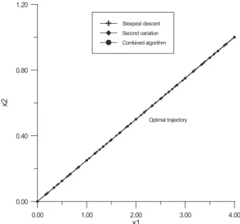
0.00 1.00 2.00 3.00 4.00 x1
0.00 0.40 0.80 1.20
x2
Optimal trajectory Steepest descent Second variation Combined algorithm
Figure 3. Optimal trajectory for Zermelo problem.
Brachistochrone problem
One of the most famous issue in the Mathematics history is the Brachistochrone problem, which consists of determining
the curve y([) that a m mass particle will slide from point $ to a
lower B, without friction, in the minimum time. The statement
of the problem is as follows (Williamson and Tapley, 1972;
Bryson and Ho, 1975). Determine the control u(t) that transfers
the system described by the differential equations:
u x dt dx
cos
2 1
u x dt dx
sin 2 2
1 3
dt dx
(63)
from the initial conditions:
[i(t0 ) = [i
0 ,i = 1, 2, 3, (64)
WRWKH¿QDORQHV
[1(tf) = [1
f [
2(tf) = free, (65)
and minimizes the performance index:
J = [3(tf). (66)
In order to solve this time-free problem by means of the algorithms of the steepest descent and the second variation methods, one proceeds as described in the previous section.
Introducing a new independent variable IJ, IJ[0,1] and an
auxiliary control variable Į through the equation 67
t = ĮIJ, (67)
WKHWLPHIUHHSUREOHPGH¿QHGE\(TVWRLVFRQYHUWHG WRDWLPH¿[HGSUREOHPZLWKVWDWHHTXDWLRQVJLYHQE\(T
u x d
dx
cos
2 1
D
W d x u
dx
sin
2 2
D
W dW D
dx3
. (68)
The penalty function method (Hestenes, 1969; O’Doherty and Pierson, 1974) must be used in order to apply the algorithm of the steepest descent method derived for a Mayer problem
ZLWK IUHH ¿QDO VWDWH 7KH QHZ WLPH¿[HG SUREOHP LV WKHQ GH¿QHGE\WKHVWDWHHTXDWLRQVWKHLQLWLDOFRQGLWLRQV
and a new performance index obtained from Eqs. 65 and 66:
21 1 1 3(1) (1)
f
x x k x
J , (69)
where k1>>1 must be chosen by the user of the algorithm.
Both methods use the partial derivatives of the Hamiltonian
function H, which is given by Eq. 70:
>
@
>
2 O1cos O2sin O3@
D x u u
H
.
(70)As an example, consider the following boundary conditions (Williamson and Tapley, 1972):
[1(0) = 0.015134313 [2(0) = 0.059647112
[3(0) = 0.5 [1(1) = 1.0 .
The exact solution to these boundary conditions is
[2(tf)=0.634974 and [3(tf 7KH¿UVWDSSUR[LPDWLRQ
of the control variables is chosen as Eqs. 71 and 72 for the two algorithms.
u(IJ) = 0.5, IJ[0,1], (71)
Į(IJ) = 1.5, IJ[0,1], (72)
The numerical results are shown in Table 2. In both cases,
the convergence criterion is given by
|
I3n+1 - I3n|
< 1.0×10⁻⁶.The numerical results are obtained taking: k1 = k2 = 1000;
ȕ = 0.95; K0 = 0.02; L = 400, for the steepest descent method,
and k = 0.25; İ = 0.75; Wii,2 = -2000, for the second variation
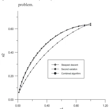
method requires less iterations than the steepest descent method, but the accuracy of the solution is worse. In Fig 4, the rates of convergence for steepest descent and second varia-tion methods are presented. For the steepest descent method, Fig. 4 shows an oscillatory behaviour, which is produced by the change of the step size in control space. Figures 5 and 6 shows the time history of the optimal control and trajec-tory for both methods. For the sake of simplicity, [2- axis is upwards. The results for the combined algorithm are also presented in Table 2. It should be noted that the algorithm converges in less iterations and presents a good accuracy of
WKHVROXWLRQ7KHRVFLOODWRU\EHKDYLRXULQWKH¿UVWLWHUDWLRQV
shown in Fig. 4 is produced by the change of the step size
LQFRQWUROVSDFHLQWKH¿UVWVWDJHRIWKHDOJRULWKPVWHHSHVW
descent method).
Table 2. Numerical results for Brachistochrone problem. Optimization
method J [1(1) [2(1)
Number of iterations |ǻI3| Steepest
descent 2.0063 0.9993 0.6382 477 5.97×10 -4
Second
variation 2.0363 0.9999 0.6463 59 2.94×10 -2
Combined
algorithm 2.0070 1.0000 0.6293 20 6.00×10 -5
0 40 80 120 160
Number of iterations 1.40
1.60 1.80 2.00 2.20
Pe
rf
o
rm
a
n
ce
in
d
e
x
-x3
(t
f)
Second variation
Combined algorithm
Steepest descent
Figure 4. Convergence rate of the steepest descent method
for Brachistochrone problem.
0.00 0.20 0.40 0.60 0.80 1.00
Normalized time
0.00 0.40 0.80 1.20
Co
n
tr
o
lv
a
ri
a
b
le
(r
a
d
ia
n
s)
Steepest-descent Second variation Combined algorithm
Figure 5. Time history of optimal control for Brachistochrone
problem.
0.00 0.40 0.80 1.20
x1
0.00 0.20 0.40 0.60
x2
Steepest descent Second variation Combined algorithm
Figure 6. Optimal trajectory for Brachistochrone problem.
APPLICATION TO SPACE TRAJECTORIES OPTI-MIZATION TRANSFER BETWEEN COPLANAR CIRCULAR ORBITS
Low-thrust limited power propulsion systems are
char-DFWHUL]HGE\ORZWKUXVWDFFHOHUDWLRQOHYHODQGKLJKVSHFL¿F
dt J
t
t
³
02
2 1
J , (73)
where Ȗ is the magnitude of the thrust acceleration vector Ȗ, used as a control variable. The consumption variable J is a monotonic decreasing function of the mass m of the space
vehicle:
¸¸¹ · ¨¨©
§
0 max
1 1
m m P
J , where 3
max is the maximum
power and m0 is the initial mass. The minimization of the
¿QDOYDOXHJf is equivalent to the maximization of mf or the minimization of the fuel consumption.
The optimization problem concerning simple transfers (no rendezvous) between coplanar orbits is formulated as: at time
t, the state of a space vehicle MLVGH¿QHGE\WKHUDGLDOGLVWDQFH r from the center of attraction, the radial and circumferential components of the velocity, u and v, and the fuel consumption
J. In the two-dimensional formulation, the state equations are given by Eq. 74:
(74)
R r r v
dt du
2
2
P
S
r
uv
dt
dv
u
dt
dr
2 22
1
S
R
dt
dJ
,where, ȝ is the gravitational parameter, R e S are, respectively, radial and circumferential thrust acceleration vectors, from initial conditions t0
u(0) = 0 v(0) = 1 r(0) = 1 J(0) = 0, (75)
WR¿QDOVWDWHVLQtf
0
)
(
t
fu
f f
r t
v( )
P
r
(
t
f)
r
f, (76)such that Jf be minimum. The performance index is given by Eq. 77:
I3 = J(tf). (77)
All variables are taken nondimensionally and we suppose there are no restrictions in the acceleration vector.
As an example of the application of the proposed method for orbit transfer problem described, consider Figs. 7 and 8, which present the consumption variable J as function of
1
0 ! r rf
U and ȡ<1, respectively, for nondimensional times of
ÀLJKWWZRWR¿YH
t=4
t=5 t=2
t=3
U
Proposed algorithm Linear theory
0.01 0.10 1.00
0.00
0.00
0.00
1.00 1.20 1.40 1.60
Jf (log)
Figure 7. Consumption for ȡ>1DQGQRQGLPHQVLRQDOWLPHRIÀLJKW
from 2 to 5.
t=2
t=3
t=4
t=5
U
Proposed algorithm Linear theory
0.01 0.10
0.00
0.00
0.00
0.70 0.80 0.90 1.00
Jf (log)
Figure 8. Consumption ȡ >1 and non-dimensional time of
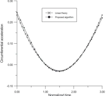
7KHVH¿JXUHVSUHVHQWDOVRDFRPSDULVRQEHWZHHQWKHUHVXOWV
obtained with the proposal algorithm (combined algorithm) and a linear theory (Silva Fernandes and Golfetto, 2007). One can verify that the curves match almost precisely, presenting good agreement between the numerical and analytical results. The method provides a good approximation for the solution of low-thrust limited power transfer to coplanar circular orbits in a central Newtonian gravitational
¿HOGSUREOHPV,WFDQEHQRWHGWKDWWKHELJJHUWKHGLIIHUHQFHEHWZHHQ LQLWLDODQG¿QDOUDGLLWKHELJJHULVWKHIXHOFRQVXPSWLRQ
In Figs. 9 and 10, respectively, one can verify the radial and circumferential acceleration evolutions for tf - t0 = 3 and
ȡ= 1.523 (Earth-Mars).
0.00 1.00 2.00 3.00
Normalized time -0.40
-0.20 0.00 0.20 0.40
Ra
d
ia
la
cc
e
le
ra
tio
n
Linear theory
Proposed algorithm
Figure 9. Radial acceleration history for ȡ=1.523 and tf-t0= 3.
0.00 1.00 2.00 3.00
Normalized time -0.10
0.00 0.10 0.20 0.30
Ci
rc
u
m
fe
re
n
tia
la
cc
e
le
ra
tio
n
Linear theory
Proposed algorithm
Figure 10. Circumferential acceleration history forȡ=1.523 and
tf-t0= 3.
CONCLUSIONS
In this paper, two classic direct methods – steepest descent and second variation – for computing optimal trajectories are reviewed, and the main advantages and disadvantages of these methods are discussed. An algorithm that combines the good characteristics of each method is also presented. The algorithms are applied for solving two classic optimization problems: Zermelo and Brachistochrone problems. Finally, the proposed algorithm is used to solve the problem of optimization of space trajectories transference between coplanar circular orbits with
D¿[HGWLPH,WKDVEHHQGHPRQVWUDWHGWKHJRRGDSSUR[LPDWLRQ
that the algorithm can provide.
ACKNOWLEDGEMENTS
This research has been supported by the Brazilian National Counsel of Technological and Scientific Development (CNPq), under contract 302949/2009-7.
REFERENCES
Betts, J.T., 1994, “Optimal Interplanetary Orbit Transfers by Direct Transcription”, The Journal of the Astronautical Sciences, Vol. 42, No. 3, pp. 247-268.
Betts, J.T., 1993, “Using Sparse Nonlinear Programming to Compute Low Thrust Orbit Transfers”, The Journal of the Astronautical Sciences, Vol. 41, No. 3, pp. 349-371.
Bliss, G.A., 1946, “Lectures on the Calculus of Variations”, University of Chicago Press, Chicago, 296 p.
Bryson, A.E., Ho, Y.C., 1975, “Applied Optimal Control”, John Wiley & Sons, New York, 481 p.
Bryson, A.E., Jr., Denham, W.F., 1962, “A Steepest Ascent Method for Solving Optimum Programming Problems”, Journal of Applied Mechanics, Vol. 84, No. 3, pp. 247-257.
Coverstone-Carroll, V., Williams, S.N., 1994, “Optimal Low Thrust Trajectories Using Differential Inclusion Concepts”, The Journal of the Astronautical Sciences, Vol. 42, No. 4, pp. 379-393.
Elsgolts, L., 1977, “Differential Equations and the Calculus of Variations”, Mir Publishers, Moscow, 440 p.
Gelfand, I.M., Fomin, S.V., 1963, “Calculus of Variations”, Prentice-Hall, New Jersey, 232 p.
Hestenes, M. R., 1969, “Multiplier and gradient methods”, Journal of Optimization Theory and Applications, Vol. 4, No. 5, pp. 303-320.
Hestenes, M. R., 1966, “Calculus of Variations and Optimal Control Theory”, John Wiley & Sons, New York, 405 p.
Hussu, A., 1972, “The Conjugate-gradient Method for Optimal Control Problems with Undetermined Final Time”, International Journal of Control, pp. 79-82.
Imae, J., 1998, “A Riccati-equation-based Algorithm for Continuous Time Optimal Control Problems”, Optimal Control Applications & Methods, Vol. 19, No. 5, pp. 299-310.
Kelley, H.J., 1960, “Gradient Theory of Optimal Flight Paths”, ARS Journal, Vol. 30, pp. 947-953.
Lasdon, L.S. et al., 1967, “The Conjugate Gradient Method
for Optimal Control Problems”, IEEE Transactions on Auto-matic Control, Vol. AC-12, No. 2, pp. 132-138.
Leitmann, G., 1981, “The Calculus of Variations and Optimal Control – An Introduction”, Plenum Press, New York, 311 p.
Longmuir, A.G. and Bohn, E.V., 1969, “Second-Variation Methods in Dynamic Optimization”, Journal of Optimization Theory and Applications, Vol. 3, No. 3, pp. 164-173.
Marec, J. P., 1976, Optimal space trajectories. New York, Elsevier, 329 p.
McDermott, Jr., M., Fowler, W.T., 1977, “Steepest-Descent Failure Analysis”, Journal of Optimization Theory and Appli-cations, Vol. 23, No. 2, pp. 229-243.
McGill, R., Kenneth, P., 1964, “Solution of Variation Prob-lems by Means of a Generalized Newton-Raphson Operator”, AIAA Journal, Vol. 2, No. 3, pp. 1761-1766.
McIntyre, J.E., 1968, “Guidance, Flight Mechanics and Trajectory Optimization. Vol. XIII – Numerical Optimization Methods”, NASA CR – 1012, 105 p.
O’Doherty, R.J., Pierson, B.L., 1974, “A Numerical Study of Augmented Penalty Function Algorithms for Terminally Constrained Optimal Control Problems”, Journal of Optimi-zation Theory and Applications, Vol. 14, No. 4, pp. 393-403.
Pontryagin, L.S. et al., 1962, “The Mathematical Theory
of Optimal Control Processes”, John Wiley & Sons, New York, 357 p.
4XLQWDQD9+'DYLVRQ(-³$QXPHULFDOPHWKRG IRUVROYLQJFRQWUROSUREOHPVZLWKXQVSHFL¿HGWHUPLQDOWLPH´
International Journal of Control, Vol. 17, No. 1, pp. 97-115.
Sage, A.P., White, C.C., 1977, “Optimum Systems Control”, 2nd edition, Prentice – Hall Inc., Englewood Cliffs, New Jersey, 413 p.
Seywald, H., 1994, “Trajectory Optimization Based on Differ-ential Inclusion”, Journal of Guidance, Control and Dynamics. Vol. 17, No. 3, pp. 480-487
Silva Fernandes, S., Golfetto, W. A., 2007, “Numerical computation of optimal low-thrust limited-power trajectories-transfer between coplanar circular orbits”, Mathematical Problems in Engineering.