Braz. J. Chem. Eng. vol.28 número2

(1)

ISSN 0104-6632 Printed in Brazil

www.abeq.org.br/bjche

Vol. 28, No. 02, pp. 325 - 332, April - June, 2011

Brazilian Journal

of Chemical

Engineering

VAPOR-LIQUID EQUILIBRIUM MEASUREMENTS

FOR THE BINARY SYSTEM METHYL

ACETATE+ETHANOL AT 0.3 AND 0.7 MPa

P. Susial

*

, R. Rios-Santana and A. Sosa-Rosario

Escuela Técnica Superior de Ingenieros Industriales, Phone: 928-458658, Universidad de Las Palmas de Gran Canaria, 35017 Tafira Baja,

Las Palmas de Gran Canaria - Islas Canarias, España. E-mail: psusial@dip.ulpgc.es

(Submitted: February 3, 2010 ; Revised: February 7, 2011 ; Accepted: February 11, 2011)

Abstract - This paper reports experimental data of the isobaric vapor-liquid equilibria (VLE) for the mixture

methyl acetate + ethanol at 0.3 and 0.7 MPa, determined using a copper still ebulliometer. The activity coefficients obtained from the experimental data were correlated by using different thermodynamic mathematical models. All the binary systems show a positive consistency when subjected to the point-to-point test of Van Ness. The prediction of VLE data obtained with the UNIFAC and ASOG methods has been verified with experimental data.

Keywords: VLE isobaric data; Activity coefficient; Methyl ester; Ethanol.

INTRODUCTION

Previous papers (Ortega and Susial, 1990; Ortega and Susial, 1993) have reported VLE data for methyl esters and alkanols at different pressures. The methyl acetate + ethanol binary system was reported at isothermal conditions of 323.15 K, 333.15 K, 343.15 K and 353.15 K by Perelygin and Volkov (1970) (see Gmehling and Onken, 1986). This system has also been reported at isobaric conditions by Perelygin and Volkov (1970) and Nishi (1972) (see Gmehling and Onken, 1986) and by Ortega et al. (1990) at 101.3 kPa, while Ortega and Susial (1990) have published data for the methyl acetate + ethanol system at 114.66 kPa and 127.99 kPa. In the present work, VLE measurements of methyl acetate + ethanol at 0.1, 0.3 and 0.7 MPa obtained with a copper still are presented.

The experimental data of this paper at 0.1, 0.3 and 0.7 MPa were verified thermodynamically using the point-to-point test of Van Ness (Van Ness et al., 1973) and by applying the procedure of Barker

(Barker, 1953) implemented in the computer program of Fredenslund et al. (1977).

All data included in this work have passed the consistency test according to the Fredenslund criteria (Fredenslund et al., 1977). These data were used to check the reliability of UNIFAC (Fredenslund et al., 1977; Fredenslund et al., 1975; Gmehling et al., 1993; Larsen et al., 1987) and ASOG (Kojima and Tochigi, 1979) group contribution models in order to expand the applicability of these predictive models.

EXPERIMENTAL

Materials and Apparatus

(2)

326 P. Susial, R. Rios-Santana and A. Sosa-Rosario

Brazilian Journal of Chemical Engineering

point at 0.1 MPa was determined with the copper ebulliometer. A Kyoto Electronics DA-300 vibrating tube density meter with an uncertainty of ±0.1 kg•m-3 and a Zusi model 315RS Abbe refractometer with an uncertainty of ±0.0002 units were used for density and refractive index determinations, respectively. The measures of the pure substance properties are compared with literature values.

VLE Equipment and Procedure

A still ebulliometer developed and built in copper, with all its different pieces assembled with silver-weldings is presented in Figure 1. The still has a configuration similar to the apparatus made of glass by de Afonso et al. (1983). The equipment has a double-walled inverted vessel where a boiling mixture of liquid and vapor is generated by an electric heater. This boiling mixture rises in a tube that works like a Cotrell pump. The Cotrell tube is connected to a vessel that acts like an equilibrium

chamber. The liquid and vapor phases are carried out on separate paths from this equilibrium chamber. A tube connected to a funnel collects and circulates the liquid phase in the equipment. This tube has a lateral path that ends in a valve. The vapor phase is carried out to the cooler. The cooler has a coaxial tube that returns the condensate to the still and it has a lateral path with a finishing valve. Therefore, both phases are refluxed.

The equilibrium equipment has been designed to work at moderate pressures. Therefore, slight modifications were made to this copper still in order to ease sampling of both phases at the working pressures (see Figure 1). Some airtight outer vessels must be used. In addition, it was necessary to prepare J-type thermocouples with a ring silver-soldered to both its cover and the ebulliometer. Thermocouples of Thermocoax (range 1073 K) with 0.1% precision were used for the temperature measurements. The working pressure was measured with a NuovaFima manometer with a range from 0 to 1.0 MPa and 1% precision.

Table 1: Physical properties of pure compounds at atmospheric pressure

Tbp/K ρ (298.15 K)/(kg•m-3) nD (298.15 K)

purity/mass%

exp lit exp lit exp lit

ethanol puriss. p.a. > 99.9 351.35

351.443 (A) 351.45 (B) 351.44 (C)

785.2 784.93 (A)

785.2 (B) 1.3600

1.35941 (A) 1.3594 (B,C)

methyl acetate puriss. > 99 330.05

330.018 (A) 329.95 (B) 330.09 (C)

927.3 927.90 (A)

927.30 (B) 1.3590

1.3589 (A,C) 1.3587 (B)

(A) Riddick et al., 1986; (B) Nagata et al., 1976; (C) Yaws, 2003

T1,T2 - Thermocouples A - boiling flask B - outlet valve C - vapor sampler D - liquid sampler E - heater F - cooler G - inlet valve

(3)

The copper still described in this paper showed good agreement with the ebulliometer previously used, the operation procedure also being similar (de Afonso et al., 1983; Ortega et al., 1990; Susial et al., 1989). The procedure differs in the residence time of the mixture inside the ebulliometer and the sampling method. The ebulliometer has a 400 cm3 mixture capacity, the reason why a 90 min recirculation time is necessary for the mixture. This was evaluated by a previous test of operation time vs. mole fraction of both phases (de Afonso et al., 1983). Samples of the liquid and vapor phases were removed from the airtight vessels with syringes and the compositions of the equilibrium phases were obtained by densimetry at 298.15 K, using a composition-density standard curve prepared for the mixture studied in this paper,

2 3

1 1 1

785.2 181.1 x• 51.5 x• 12.5 x•

ρ = + − + (1)

As in previous works (Ortega et al., 1990; Ortega and Susial, 1990; Susial et al., 1989), the values of the data pairs composition-density were correlated by using the Nelder and Mead (1967) procedure. Therefore, considering the different apparatus used, the estimated accuracy in the determination of both the liquid and vapor phase was better than ±0.002 units of mole fraction.

RESULTS AND TREATMENT

With the copper still ebulliometer, the experimental T-x1-y1 data (Table 2) for methyl acetate+ethanol were obtained at 0.1, 0.3 and 0.7 MPa. Also included in Table 2 are the activity coefficients of the liquid phase for each system, calculated by using the following equation:

( )

o L

i i i i

i o o i i i

p p v

y p exp

RT

x p

⎡ ₋ ⎤

ϕ _⎢ _⎥

γ =

⎢ ⎥

ϕ _⎣ _⎦ (2)

The fugacity coefficients were calculated by using the virial state equation truncated at the second term, and from the following equation:

i i ij i j ij j i j

p

exp 2 y B y y B

RT

⎡ ⎛ ⎞⎤

⎢ ⎜ ⎟⎥

ϕ = _⎢ _⎜ − _⎟_⎥

⎝ ⎠

⎣

∑

∑∑

⎦

(3)

The second virial coefficients were calculated by the Hayden and O’Connell (1975) method. The liquid molar volumes of the pure compounds were estimated by the equation of Yen and Woods (1966).

VLE experimental data in this paper were verified by using the thermodynamic consistency test of Van Ness et al. (1973). The proposed computer program

of Fredenslund et al., (1977) was applied using physical properties from the literature (Fredenslund et al., 1977; Riddick et al., 1986; Yaws, 2003) and the correlations of the vapor pressures from a previous paper (Susial et al., 2010).

All the systems included in this work passed the point-to-point test because they have an average deviation of δ(y1) < 0.01 (Fredenslund et al., 1977). The experimental data (Table 2) were correlated by using the calculated activity coefficients in the form of GE/RT vs. x1 with the Redlich-Kister, Van Laar, Margüles, Wilson, NRTL and UNIQUAC models. To calculate the constants of each model, a non-linear regression procedure was employed (Nelder and Mead, 1967), considering a minimization of the objective function (OF) (Holmes and Winkle, 1970; Postigo et al., 2009):

(

)

2

(

)

2

n n

exp calc exp calc

1 2

1 1

OF=

∑

γ − γ +

∑

γ − γ (4)

The results of the correlations with thermodynamic mathematical models are presented in Table 3. The models give good fit to the experimental data and show acceptable mean deviations for the prediction of the vapor phase composition.

In addition, as in previous papers (Ortega et al., 1990; Ortega and Susial, 1990; Susial et al., 1989), the experimental data of each system were correlated to a fitting function (FF) with a polynomial form (see Table 4). Results of the experimental data treatment with the different FF, using the Nelder and Mead (1967) procedure to minimize the summation of the square of the deviations, are shown in Table 4.

A mathematical treatment similar to literature data (Ortega et al., 1990; Ortega and Susial, 1990) was made for the parameter of interest (y1-x1) or T. The fits of the experimental data of this paper (Table 4) are plotted in Figure 2 and 3, respectively).

(4)

Table 2: VLE experimental data and calculated values of activity coefficients of the liquid phase

T/K x1 y1 γ1 γ2

methyl acetate (1) + ethanol (2) at 0.1 MPa

351.35 0.000 0.000 1.000

349.05 0.038 0.127 1.789 0.979 345.95 0.079 0.254 1.892 0.991 341.35 0.168 0.418 1.691 1.037 339.75 0.211 0.496 1.681 1.014 337.25 0.291 0.577 1.538 1.056 336.75 0.335 0.602 1.417 1.083 336.05 0.372 0.635 1.377 1.084 334.45 0.441 0.686 1.323 1.125 333.75 0.488 0.703 1.254 1.199 332.95 0.569 0.738 1.160 1.302 331.95 0.643 0.773 1.112 1.425 331.55 0.686 0.791 1.081 1.519 331.15 0.720 0.809 1.068 1.586 330.45 0.855 0.874 0.995 2.085 330.25 0.874 0.892 1.000 2.075 330.15 0.902 0.911 0.993 2.208 330.15 0.911 0.921 0.994 2.158 329.95 0.959 0.959 0.990 2.453 330.05 1.000 1.000 1.000

382.05 0.000 0.000 1.000

380.65 0.018 0.064 2.387 0.985 378.65 0.058 0.162 1.972 0.980 375.15 0.141 0.313 1.715 0.989 374.15 0.168 0.350 1.652 0.999 372.35 0.225 0.418 1.544 1.020 371.45 0.254 0.449 1.504 1.034 370.45 0.291 0.481 1.444 1.061 370.35 0.320 0.512 1.402 1.043 367.75 0.465 0.610 1.233 1.159 367.45 0.496 0.635 1.213 1.164 366.95 0.536 0.652 1.168 1.226 365.65 0.627 0.703 1.115 1.363 365.05 0.703 0.756 1.088 1.436 364.15 0.892 0.892 1.037 1.802 364.45 0.950 0.940 1.018 2.138 364.55 0.979 0.969 1.015 2.619 365.25 1.000 1.000 1.000

410.75 0.000 0.000 1.000

(5)

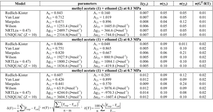
Table 3: Correlation parameters of GE/RT vs. x1, mean deviations and standard deviations

Model parameters δ(y1) σ(γ1) σ(γ2) σ(GE/RT)

Redlich-Kister A0 = 0.843 A1 = 0.160 0.007 0.05 0.05 0.01

Van Laar A12 = 0.712 A21 = 1.019 0.007 0.06 0.05 0.01

Margules A12 = 0.671 A21 = 0.896 0.008 0.04 0.12 0.01

Wilson Δλ12 = 1253.4 (J•mol-1) Δλ21 = 1605.0 (J•mol-1) 0.006 0.05 0.05 0.01

NRTL(α = 0.47) Δg12 = 2489.7 (J•mol-1) Δg21 = 366.6 (J•mol-1) 0.007 0.05 0.05 0.01

UNIQUAC (Z = 10) Δu12 = 2316.8(J•mol-1) Δu21 = -744.0 (J•mol-1) 0.007 0.05 0.05 0.01

Redlich-Kister A0 = 0.806 A1= 0.048 0.005 0.09 0.011 0.02

Van Laar A12 = 0.751 A21 = 0.865 0.005 0.10 0.10 0.02

Margules A12 = 0.820 A21 = 0.667 0.006 0.06 0.21 0.02

NRTL(α = 0.47) Δg12 = 1800.2 (J•mol-1) Δg21 = 1084.1 (J•mol-1) 0.006 0.09 0.10 0.03

UNIQUAC (Z = 10) Δu12 = 1836.6 (J•mol-1) Δu21 = -419.8 (J•mol-1) 0.005 0.10 0.10 0.02

Redlich-Kister A0 = 0.607 A1 = 0.205 0.012 0.09 0.12 0.02

Van Laar A12 = 0.426 A21 = 0.899 0.012 0.09 0.09 0.02

Margules A12 = 0.441 A21 = 0.570 0.009 0.08 0.24 0.01

NRTL(α = 0.47) Δg12 = 4244.0 (J•mol-1) Δg21 = -970.3 (J•mol-1) 0.014 0.10 0.08 0.02

UNIQUAC (Z = 10) Δu12 = 3604.5 (J•mol-1) Δu21 = -1607.4 (J•mol-1) 0.012 0.09 0.10 0.02 n

exp cal 1

1

(F) F F n

δ =

∑

− ;

(

)

n 2

exp cal

1 F F

(F)

n m −

σ =

∑

₋ ; _{( )} n exp cal

exp 1

F F 100

ē F

n F −

=

∑

Table 4: Fittings coefficients for FF and standard deviations

FF RT A0 A1 A2 A3

[ ]₁

{

[ ]₁

}

k

1 1 1 1 k 1 1 T 1

k 0

(y x ) x (1 x )− A x x R (1 x )− =

− − =

∑

+ − 0.758 2.865 -5.896 5.620 -2.677 σ(y1-x1) <0.01

[ ]₁

{

[ ]₁

}

k

1 bp1 1 bp2 1 1 k 1 1 T 1

k 0

T x T (1 x )T x (1 x )− A x x R (1 x )− =

⎡ − − − ⎤ − = + −

⎣ ⎦

∑

0.267 -62.708 43.235 σ(T)/K = 0.25

[ ]₁

{

[ ]₁

}

k

1 bp1 1 bp2 1 1 k 1 1 T 1

k 0

T y T (1 y )T y (1 y )− A x x R (1 x )− =

⎡ − − − ⎤ − = + −

⎣ ⎦

∑

2.807 4.393 -35.974 σ(T)/K = 0.22

(

)

[ ]₁

{

[ ]₁

}

k

E

1 1 k 1 1 T 1

k 0

G / RT x (1 x )− A x x R (1 x )−

=

− =

∑

+ − -0.018 1.764 -0.939 σ(GE_{/RT) < 0.01}

[ ]₁

{

[ ]₁

}

k

1 1 1 1 k 1 1 T 1

k 0

(y x ) x (1 x )− A x x R (1 x )− =

− − =

∑

+ − 0.344 2.621 -5.178 5.505 -3.107 σ(y1-x1) < 0.01

[ ]₁

{

[ ]₁

}

k

1 bp1 1 bp2 1 1 k 1 1 T 1

k 0

T x T (1 x )T x (1 x )− A x x R (1 x )− =

⎡ − − − ⎤ − = + −

⎣ ⎦

∑

1.226 -46.930 80.540 -71.950 σ(T)/K = 0.17

[ ]₁

{

[ ]₁

}

k

1 bp1 1 bp2 1 1 k 1 1 T 1

k 0

T y T (1 y )T y (1 y )− A x x R (1 x )− =

⎡ − − − ⎤ − = + −

⎣ ⎦

∑

2.285 -2.199 -36.419 σ(T)/K = 0.18

(

)

[ ]

{

[ ]

}

k

1 1

E

1 1 k 1 1 T 1

k 0

G / RT x (1 x )− A x x R (1 x )− =

− =

∑

+ − 6.640 0.608 0.768 σ(GE/RT) = 0.01

[ ]₁

{

[ ]₁

}

k

1 1 1 1 k 1 1 T 1

k 0

(y x ) x (1 x )− A x x R (1 x )− =

− − =

∑

+ − 1.181 1.180 -3.331 4.182 -2.557 σ(y1-x1) < 0.01

[ ]₁

{

[ ]₁

}

k

1 bp1 1 bp2 1 1 k 1 1 T 1

k 0

T x T (1 x )T x (1 x )− A x x R (1 x )− =

⎡ − − − ⎤ − = + −

⎣ ⎦

∑

0.239 -9.833 -98.281 199.718 -116.830 σ(T)/K = 0.18

[ ]₁

{

[ ]₁

}

k

1 bp1 1 bp2 1 1 k 1 1 T 1

k 0

T y T (1 y )T y (1 y )− A x x R (1 x )− =

⎡ − − − ⎤ − = + −

⎣ ⎦

∑

2.864 -4.576 -53.990 39.147 σ(T)/K = 0.18

(

)

[ ]₁

{

[ ]₁

}

k

E

1 1 k 1 1 T 1

k 0

G / RT x (1 x )− A x x R (1 x )− =

(6)

0 0.2 0.4 0.6 0.8 1

x1

0 0.1 0.2 0.3

y1 -x1

0.1 0.3 0.5 0.7 0.9

x1

340 360 380 400

T/

K

0 0.2 0.4 0.6 0.8 1

x1

330 340 350

T/

K

T/K = 610.35 -288.89_•x

1

Figure 2: Experimental values and fitting curves for the mixture of methyl acetate (1) + ethanol (2) at 0.1 MPa (z), 0.3 MPa () and 0.7 MPa (S). Fitting curves and the literature values for methyl acetate (1) + ethanol (2) at different pressures: (+) 101.3 kPa (Ortega et al., 1990), and (฀) 127.99 kPa (Ortega and Susial, 1990).

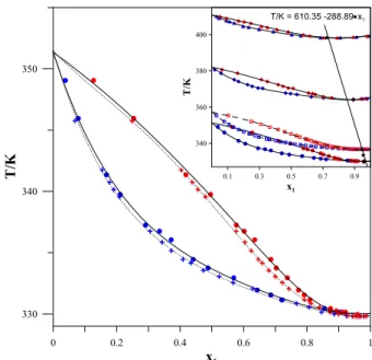
Figure 3: Experimental values and FF curves of T vs. x1 and T vs. y1 for methyl acetate (1) + ethanol (2) at 0.1 MPa (z), 0.3 MPa () and 0.7 MPa (S) compared with FF curves and the literature values for methyl acetate (1) + ethanol (2) at different pressures: (+) 101.3 kPa (Ortega et al., 1990), and (฀) 127.99 kPa (Ortega and Susial, 1990).

The experimental data from this paper at 0.1 MPa show that the methyl acetate + ethanol binary system has an azeotrope at x1az100 = y1az100 = 0.959 and Taz100 = 329.95 K. This result does not differ significantly with the literature data (Gmehling et al., 2004) due to the fact that the small difference in temperature is within the range of error of the thermocouple used in this work. On the other hand, for 0.3 and 0.7 MPa a modification in the azeotropic data is verified. For these isobaric conditions, the location of the singular point is x1az300 = y1az300 = 0.892, Taz300 = 364.15 K at 0.3 MPa; and x1az700 = y1az700 = 0.723, Taz700 = 398.25 K at 0.7 MPa. A representation of the experimental azeotropic data of this paper and the bibliografic data (Gmehling et al., 2004) shows a relation between both (Figure 3). Azeotropic data at 0.1 and 0.7 MPa show a suitable position regarding the correlation equation; however, the azeotropic data at 0.3 MPa present an error of less than 5%, as shown in the inset in Figure 3.

The UNIFAC (Fredenslund et al., 1977; Fredenslund et al., 1975; Larsen et al., 1987) group contribution method and the ASOG (Kojima and

Tochigi, 1979) model were used in previous papers (Ortega et al., 1990; Ortega and Susial, 1990; Susial et al., 1989) for the prediction of the VLE of isobaric data at pressures near atmospheric. This paper evaluates the behaviour in the prediction of VLE data by the different versions of UNIFAC and the ASOG group contribution models with respect to the experimental data obtained in this study at moderate pressures. Results are presented in Table 5.

(7)

Table 5: Mean deviations and average errors in the prediction of VLE data. Experimental and predicted azeotropic data

UNIFAC 1975 (A) COH/COO

UNIFAC 1977 (B) CCOH/COOC

UNIFAC 1987 (C) OH/COOC

UNIFAC 1993 (D) OH/COOC

ASOG 1979 (E) OH/COO methyl acetate (1) + ethanol (2) at 0.1 MPa

δ(y1) 0.01 0.01 0.01 0.01 0.01

ē(γ1) 2.71 3.23 3.55 2.42 4.39

δ(T)/K 0.36 0.76 0.33 0.38 0.45

Azeotropic data

x1az exp = 0.959 0.910 0.907 0.914 0.908 0.915

Taz exp = 329.95 K 329.83 329.79 330.14 329.83 330.17

δ(y1) 0.01 0.01 0.02 0.01 0.01

ē(γ1) 2.79 4.08 7.47 3.79 3.59

δ(T)/K 0.38 1.29 1.52 0.44 0.83

Azeotropic data

x1az exp = 0.892 0.829 0.780 0.926 0.844 0.796

Taz exp = 364.15 K 364.95 364.45 365.96 365.17 365.58

δ(y1) 0.01 0.02 0.02 0.01 0.01

ē(γ1) 5.75 11.26 7.27 3.67 8.25

δ(T)/K 1.74 3.18 1.16 1.03 2.12

Azeotropic data

x1az exp = 0.723 0.726 0.678 0.886 0.748 0.689

Taz exp = 398.25 K 396.67 395.37 399.57 397.48 397.17

(A) Fredenslund et al., 1975; (B) Fredenslund et al., 1977; (C) Larsen et al., 1987; (D) Gmehling et al., 1993; (E) Kojima and Tochigi, 1979

CONCLUSIONS

VLE data at moderate pressures have been obtained with a copper ebulliometer. Data for the methyl acetate + ethanol binary system at 0.1, 0.3 and 0.7 MPa are presented. The experimental data passed positively the consistency test of Van Ness and showed satisfactory agreement with literature data. This binary system forms an azeotrope at 0.1 MPa, which has been verified via good agreement with literature data.. It has been also verified that the azeotropic data expressed as ester mole fraction decreases with a pressure increase.

The new isobaric data obtained at moderate pressures have been used to verify the predictive behavior of several group contribution models. The predictions achieved using the UNIFAC and ASOG models were verified by the determination of the mean deviations in the vapor phase mole fraction and the mean error in the estimation of the liquid phase activity coefficient. Results show that the predictions are good for the VLE at atmospheric pressure, while higher deviations were obtained with the pressure increase. When the UNIFAC and ASOG models were used for the azeotropic data prediction, the calculated values did not show a good agreement with the experimental data from this work at moderate pressures.

NOMENCLATURE

Ak Parameter

Bij Cross second virial coefficient

m3•mol-1

ē Average error %

F Property (F = y1; F = (y1-x1); F = γ1; F = γ2; F = T/K; F = GE/RT)

GE Excess free energy J•mol-1

m Number of equation

parameters

n Number of experimental

data

nD Refractive index

pi o

Vapor pressure kPa

p Total pressure kPa

R Universal gas constant J•K-1•mol-1

RT Parameter

T Temperature K

viL Liquid molar volume m3•mol-1 x Liquid-phase mole fraction

y Vapor-phase mole fraction

Subscripts

az Azeotrope

(8)

cal Calculated exp Experimental i, j Chemical substances lit Literature 1 Ester

Greek Letters

δ Mean deviation

φ Fugacity coefficient

γ Activity coefficient

ρ Density kg•m-3

σ Standard deviation

REFERENCES

Barker, J. A., Determination of Activity Coefficients from Total Pressure Measurements. Australian J. Chem, 6, 207-210 (1953).

de Afonso, C., Ezama, R., Losada, P., Calama, M. A., Llanas, B., Pintado, M., Saenz de la Torre, A.F., Equilibrio Isobárico Líquido.Vapor. III Desarrollo y ensayo de un aparato de equilibrio de pequeña capacidad. Anales de Química de la RSEQ, 79, 243-253 (1983).

Fredenslund, Aa., Gmehling, J. and Rasmussen, P., Vapor-liquid Equilibria Using UNIFAC. A Group Contribution Model. Elsevier, Amsterdam (1977). Fredenslund, Aa., Jones, R. L. and Prausnitz, J. M., Group-Contribution Estimation of Activity Coefficients in Nonideal Liquid Mixtures. AIChE J., 21, 1086-1099 (1975).

Gmehling, J., Li, J. and Schiller, M., A Modified UNIFAC Model. 2. Present Parameter Matrix and Results for Different Thermodynamic Properties. Ind. Chem. Eng. Res., 32, 178-193 (1993). Gmehling, J., Menke, J., Krafczyk, J. and Fischer,

K., Azeotropic Data. Ed. Wiley-VCH Verlag, 2 ed. Part. 1, p. 317, Weinheim (2004).

Gmehling, J. and Onken, U., Vapor-Liquid Equilibrium Data Collection. Chemistry Data Series. Vol. I, Part. 2, pp. 330-335, Dechema, Frankfurt (1986).

Hayden, J. G. and O’Connell, J. P., A generalised method for predicting second virial coefficients. Ind. Eng. Chem. Process Des. Dev., 14, 209-216 (1975).

Holmes, M. J. and Vanwinkle, M., Prediction of Ternary Vapor-Liquid. Equilibria from Binary Data. Ind. Eng. Chem., 62, 21-31 (1970).

Kojima, K. and Tochigi, K., Prediction of Vapor-Liquid Equilibria by the ASOG Method. Kodansha Ltd., Tokyo (1979).

Larsen, B. L., Rasmussen, P. and Fredenslund, Aa., A modified UNIFAC Group-Contribution Model for Prediction of Phase Equilibria and Heats of Mixing. Ind. Eng. Chem. Res., 26, 2274-2286 (1987).

Nagata, I., Ohta, T. and Nakagawa, S., Excess Gibss Free Energies and Heats of Mixing for Binary Alcoholic Liquid Mixtures. J. of Chem. Eng. Japan, 9, 276-281 (1976).

Nelder, J. and Mead, R., A Simplex Method for Function Minimization, Comput. J., 7, 308-313 (1967).

Ortega, J., Susial, P. and de Afonso, C., VLE Measurementes at 101.32 kPa for Binary Mixtures of Methyl Acetate+ Ethanol or 1-Propanol. J. Chem. Eng. Data, 35, 350-352 (1990).

Ortega, J. and Susial, P., VLE at 114.66 and 127.99 kPa for the Systems Methyl Acetate + Ethanol and Methyl Acetate + Propan-1-ol. Measurements and Prediction. J. of Chem. Eng. Japan, 23, 621-626 (1990).

Ortega, J. and Susial, P., Vapor-Liquid Equilibria Behavior of Methyl Esters and Propan-2-ol at 74.66, 101.32 and 127.99 kPa. J. of Chem. Eng. Japan, 26, 259-265 (1993).

Postigo, M. A., Mariano, A. B., Jara, A. F. and Zurakoski, N., Isobaric Vapor-Liquid Equilibria for the Binary Systems Benzene + Methyl Ethanoate, Benzene + Butyl Ethanoate and Benzene + Methyl Hepthanoate at 101.31 kPa. J. Chem. Eng. Data, 54, 1575-1579 (2009).

Riddick, J. A., Bunger, W. B. and Sakano, T. K., Organic Solvents. 4th ed., Wiley-Interscience. New York (1986).

Susial, P., Ortega, J., de Afonso, C. and Alonso, C., VLE Measurements for Methyl Propanoate-Ethanol and Methyl Propanoate-Propan-1-ol at 101.32 kPa. J. Chem. Eng. Data, 34, 247-250 (1989).

Susial, P., Sosa-Rosario, A. and Rios-Santana, R., VLE with a New Ebulliometer: Ester+Alcohol System at 0.5 MPa. Chinese J. Chem. Eng., 18, 1000-1007 (2010).

Van Ness, H. C., Byer, S. M. and Gibbs, R. E., Vapor-Liquid Equilibrium: I. An Appraisal of Data Reduction Methods. AIChE J., 19, 238-244 (1973).

Yaws, C. L., Yaw’s Handbook of Thermodynamic and Physical Properties of Chemical Compounds. Ed Knovel, Norwich-New York (2003).