An algorithm developed for the design of reinforcement in concrete shells is presented in this text. The formulation and theory behind the develop-ment is shown, as well as results showing its robustness and capability of application on fairly large-scale structures. The design method is based on the three-layer model for reinforced concrete shell elements. A material model is also proposed in order to improve the numerical stability of the algorithm. Comparisons of single element design show that the modiications made to the material model don’t effect signiicantly the inal results while making for better numerical stability.
Keywords: reinforced concrete; shell elements; plate elements; structural design.
Um algoritmo desenvolvido para o dimensionamento de armaduras para cascas de concreto armado é apresentado neste artigo. A formulação e aspectos teóricos que fundamentam o método são apresentados assim como, os resultados que mostram a robustez e capacidade de apli-cação do algoritmo em estruturas de grande porte. O método de dimensionamento é baseada no modelo das três chapas para elementos de casca em concreto armado. Um modelo constitutivo é proposto para obter melhor estabilidade numérica no algoritmo. Comparações feitas do dimensionamento de um único elemento mostram que as modiicações do modelo constitutivo não apresentam mudanças signiicantes nos resultados enquanto proporcionam melhor estabilidade numérica.
Palavras-chave: concreto armado, dimensionamento, cascas, chapas.
An algorithm for the automatic design of concrete
shell reinforcement
Um algoritmo para o dimensionamento automático
de cascas em concreto armado
A. B. COLOMBO a
J. C. DELLA BELLA a [email protected]
T. N. BITTENCOURT a [email protected]
a Departamento de Estruturas e Geotécnica, Escola Politécnica da Universidade de São Paulo, SP, Brasil.
Received: 31 Jan 2013 • Accepted: 10 Sep 2013 • Available Online: 13 Feb 2014
Abstract
inforced concrete structures, these elements can be found in structures such as nuclear power plants, offshore structures, and tunnel linings. This document focuses on inding the necessary reinforcement for a shell or plate element subjected to membrane forces Nx, Ny, Nxy and lexural forc -es Mx, My and Mxy. In the last decades many researchers (Baumann [1], Brodum-Nielsen [2] and Gupta [3]) have proposed solutions for this type of problem. The basic idea behind these solutions is that the forces and moments are resisted by the resultant tensile forces of the reinforcement and the resultant compressive forces of the concrete blocks.
More complex models, which focus on the behavioral analysis of rein-forced shell elements, have also been developed (Scordelis [4], Hu [5], Cervera [6], Polak [7], Wang [8], Liu [9], Schulz [10] and Hara [11]). These formulations are fundamental for the development of new design techniques, on the other hand the complexity of the material models and analysis procedures involved in these, make them very dificult to apply in practical design situations.
For these situations a simpler procedure is more favorable. Gupta [3] pre-sented a general solution procedure and an automatic solution algorithm based on it and on the CEB [12] formulation was presented by Lourenço [13], these authors proposed a general method of solution, including cas-es where there is no need for reinforcement. Tomás [14] used optimiza-tion techniques to design elements using this formulaoptimiza-tion. More recently Fall [15] suggested the same algorithm to reinforce tailor-made concrete structures. The algorithm presented here is proposed as an alternative to the one presented by Lourenço [13], it diverges on the algorithm structure and some modiications were made to the material model adopted.
2. Formulation
This section will discuss the basic theoretical concepts necessary in order to comprehend the proposed algorithm.
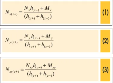
of internal stresses in the shell can be described in function of eight resultant force components shown in Figure 1. An ideal-ized shell composing of three layers is proposed by CEB [12], in this idealization the outer layers resist the bending moments and membrane forces acting on the shell and the inner layer resists the transverse shear.
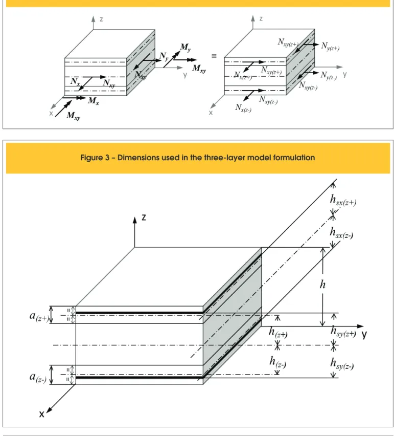
The membrane forces for the outer layers of the model can be found by applying equilibrium between the shell’s membrane forces and bending moments and the membrane forces for the outer layers, as shown in Figure 2. Equations (1) - (6) are obtained through this equilibrium, in these equations, h(z+), h
(z-), hsx(z+), hsy(z+), hsx(z-) and hsy(z-) are the indicated dimensions in
Figure 3.
(1)
(2)
)
(
( ) ( )) ( )
(
-+
-+
+
+
=
z z
y z
y z
y
h
h
M
h
N
N
(3)
(
6)
As shown in Figure 2, the three-layer model can be thought of as being comprised of two membrane elements that resist the acting forces of the shell. A problem with this idealization is that, for this to be true, the reinforcement must always be in the mid-plane of the membranes, which is often not the case. This issue is overcome by correcting the reinforcement values
(4)
(5)
Figure 2 – Equilibrium between membrane forces in the outer layers and the shell active forces
2.2 Reinforcement for membrane elements
As shown in the previous item, determining the necessary reinforce-ment for membrane elereinforce-ments is an essential part of the solution for the three-layer model. Reinforcement in membrane elements has been studied by many authors including Baumann [1], Brodum-Nielsen [2] and Gupta [16]. The design method proposed by the structural code CEB [12] incorporates the main ideas proposed by these authors. The formulation shown below is derived for a generic membrane element shown in Figure 5, of thickness a. These equa-tions can be applied to both the top (z+) and bottom (z-) membranes. Gupta [16] shows that by using the principal of minimum resis-tance it’s possible obtain the following governing equations for the and membrane forces in order to account for the real
reinforce-ment depth.
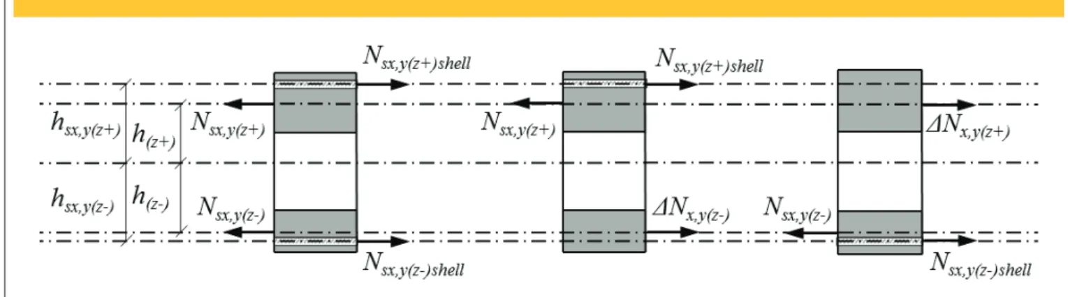
The real forces acting on the reinforcement can be found by impos-ing equilibrium between the calculated values at the mid-plane of the membrane and the values at the real position of the reinforce-ment, as shown in Figure 4, this provides the following equations for the real reinforcement values.
(7)
(
)
(
)
(
,( ) ,( ))
) ( ) ( , ) ( , ) ( ) ( , ) ( , ) ( , + -+ -+ ++
-×
+
+
×
=
z y sx z y sx z z y sx z y sx z z y sx z y sx shell z ysx
h
h
h
h
N
h
h
N
N
(8)
shell z y sx z y sx z y sx shell z ysx
N
N
N
N
, (-)=
, ( +)+
, ( -)-
, ( +)In the case where there is no membrane reinforcement in one of the layers, it’s possible to ind a correction value for the membrane forces as shown in Figure 4, based on this we ind the following equations.
(9)
(
)
(
( ) , ( ')
) ( ) ( ) ( , ) ( , -+ + ++
+
×
=
x y sx z z z z y sx shell z ysx
h
h
h
h
N
N
(10)
These equations are an important part of the proposed algorithm because the correction factor ΔN changes the membrane forces in a given layer, making it necessary to ind new reinforcement values for this layer. These new values need to be corrected again to ac-count for the real reinforcement position, creating in some cases an iterative process, this will be discussed in a latter part of this text.
Figure 4 – Equilibrium conditions used to find the correct reinfocement force
mechanical behavior of membrane elements with reinforcement in two orthogonal directions.
(13)
(1
4)
(1
5)
The optimal design is obtained for θ = 45°, so long as Nsx > 0 and Nsy > 0, meaning that the reinforcement is needed in both x and y directions. This case will be referred to as Case I, applying the θ
value above to eq. (13)-(15) yields the following equations.
(16)
(1
7)
(18)
Where Nsx and Nsy are the force by unit length in the reinforcement in the x and y directions, Nc is the force per unit length, acting on the concrete parallel to the crack. If eq.(16) gives a negative value for Nsx, setting Nsx = 0 to this equation gives the following equations which constitute Case II.
(1
9)
(
2
0)
(21)
(22)
In a similar form if eq. (14) yields a negative value for Nsy, its’ pos -sible to obtain the following equations for Case III.
(2
3)
(24)
(2
5)
(2
6)
If eq. (20) or (23) result in a negative value no reinforcement is needed. This case will be referred to as Case IV. The concrete force Nc in this case is the minimum principal force Nc2, also the maximum principal stress Nc1 has to be less than or equal to zero. The equations for the principal forces acting on the membrane are stated below.
(27)
(28)
(2
9)
(30)
When working with the three-layer model, the solution to the nec-essary reinforcement problem is inding the thickness of the outer layers. This thickness is found by dividing the compression force acting parallel to the crack direction of the concrete membrane Nc by a limit stress, the evaluation of this limit stress will be described in the next item. Eq. (31) may be used to ind the thickness of the layer.
(3
1)
2.3 Material properties
Due to the high complexity of concrete a full description of the ma-terial behavior would imply in the use of a great amount of vari-ables. For design purposes CEB [12] suggests values for average concrete strength based on the state of cracking of the structural element. In uncracked zones, the average concrete strength is given by fcd1 in eq.(32).
(3
2)
For concrete subjected to biaxial compression, fcd1 may be in-creased by the factor K given below,
(33)
where α = σ1/σ2 and σ1 and σ2 are the principal stresses at failure. For cracked zones the average strength is given by fcd2 in eq. (34).
(34)
The simplicity of the above model makes it ideal for practical use in structural design. A more complex model that represents the behavior of concrete in a better manner was presented by
Vec-chio [17]. This model was based on experimental results from re-inforced concrete panels. In this model the maximum compressive strength decreases as the maximum tensile strain ε1 increases, this compression softening equation is shown in eq. (35).
(3
5)
The material model proposed in this paper adapts the above ex-pression to interpolate between the values given by the CEB. In this model as ε
1 increases, the compressive strength is reduced
from the value given by eq. (32) down to a minimum value given by expression (34). When the element is subjected to biaxial com-pression the increase in the concrete strength given by eq. (33) is considered. Equations (36)-(38) give a mathematical representa-tion of the proposed model.
(36)
(
0
.
6
0
.
85
)
1
.
0
,
)
(
34
.
0
8
.
0
0
.
1
1
£
£
×
-=
b
b
e e
cp
(37)
1
III
-I
Cases
f
c= b
×
f
cd(38)
/IV
Case
f
c=
K
�
f
cdIn order to use this model, it is necessary to be able to estimate
ε1 at failure for a membrane element. The study of the state of
strain in membrane elements had great contributions by Gupta [16], the author presents equations (39) and (40) where the strains in the x and y reinforcements are related to the principal strains, ε1 and ε2, and the crack angle,θ. For more information
on the development of these equations the reader may refer to Chen [18].
(39)
(40)
Using these equations it’s possible to ind ε1 by estimating values
where the reinforcement is needed in both the directions, setting
ε2 = εcp (where εcp is the concrete peak compression strain), εsx= εyi
(where εyi is the steel yield strain), θ = 45°, and substituting these values in eq. (39) yields eq. (41). The same result is obtained using a similar approach with eq. (40).
(41)
For Case II setting ε2= εcp and εsx= εyi in eq. (39) yields eq. (42). Working in a similar form with Case III we obtain eq.(43) from eq. (40). The ε1 value in the equations below can be obtained from equations (22) and (26) for Case II and Case III, respectively.
(42)
(43)
Finally for Case IV ε1 is set to zero, this is done in order to obtain concrete strength value equal to fcd1.
3. Algorithms
The main objective of this procedure is inding the thickness of the outer layers of the three-layer model. In Appendix A three algo-rithms are presented, Algorithm 1 is the main algorithm and it calls the other two algorithms.
Algorithm 1 establishes an initial value for a(z+) and a(z-), cal-culates membrane forces acting on the outer layers and uses Algorithm 2 to evaluate the reinforcement forces for the outer membranes. These initial estimates for the reinforcement forc-es are inputted into Algorithm 3, this procedure reevaluatforc-es the membrane forces and reinforcement forces to take into ac-count the difference between the position of the mid-plane of the outer layers and the actual reinforcement position. Using the values of Nc(z+) and Nc(z-), new thickness values a(z+) and a(z-) are obtained. This procedure is repeated until the thickness values converge.
To better illustrate the algorithms a numerical example is given in Appendix B. A complete iteration for element 3 from Table 2 is shown in the appendix.
4. Results
A computer routine that implements the algorithm shown in the previous item was developed using the Java programming lan-guage. Elements A and B, described below, were processed by Lourenço [13]. Comparisons between the results presented by these authors with the results obtained by the algorithm proposed here are shown in Table 1.
Element A
Element B
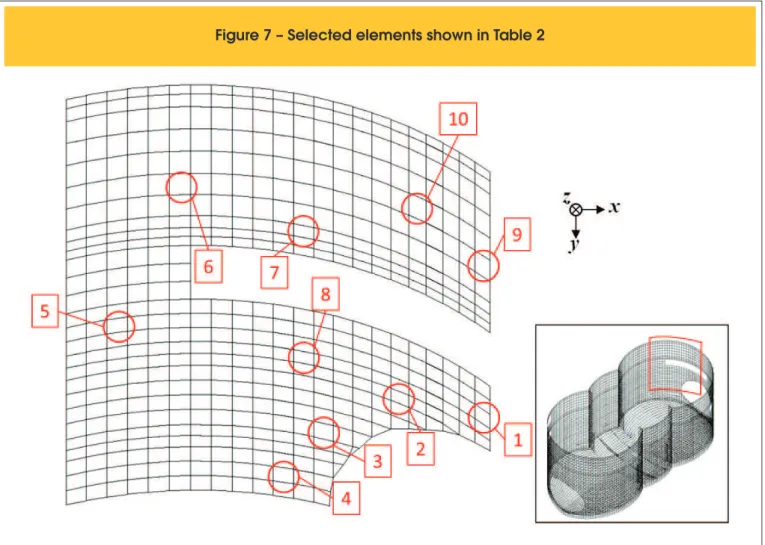
With the computer program developed it is also possible to ind reinforcement values for processed inite element models. The program was used to design the reinforcement for a model of a subway station. The contour maps in Figure 6 show the reinforce-ment results for this model, in order to present numerical results for this model, some elements were chosen (see Figure 7) and the results for these elements are shown in Table 2.
5. Conclusions
Shell-type elements can be used to model a large number of struc-tures, for a designer, being able to determine the necessary rein-forcement and check the concrete tension for these elements is fundamental. The three-layer model is a simpliied model that has been adopted by structural codes such as the CEB Model Code 1990 [12]. The fundamental concept of this model is that internal forces of two outer membranes resist the shell’s active forces. The presented procedure calculates trough an iterative method the thickness of these outer membranes, and therefore the necessary reinforcement.
The material model presented incorporates aspects of the CEB model and the compression softening model by Vec-chio [17]. This was done in order to improve convergence of the algorithm, since the discontinuity introduced by the CEB model when the material goes from an uncracked state to a cracked state caused numerical difficulties. Using the com-pression softening equation it was possible to introduce some continuity to the material model which resulted in a much more stable behavior.
Results on Table 1 show a comparison between this algorithm and the one presented by Lourenço [13]. Both results are in equilibrium with the applied forces and the reinforcement values are consis-tent. For practical use in engineering the two methods yield basi-cally the same results.
2
Figure 6 – Reinfocement area results for finite element model (Units: cm /m)
problems signiicantly but there is still plenty of room for improve -ment. Another aspect that should be mentioned is the lack of displacement compatibility in the shell formulation. These issues should be studied in future works on the area.
6. References
[01] T. Baumann, “Zur Frage der Netzbewehrung von Flächen-tragwerken,” Der Bauingenieur, vol. 47, no. 10, pp. 367-377, 1972.
[02] T. Brodum-Nielsen, “Optimum Design of Reinforced Con-crete Shells and Slabs,” Copenhagen, 1974.
[03] A. K. Gupta, “Combined Membrane and Flexural Reinforce-ment in Plates and Shells,” Journal of Structural Engineering - ASCE, vol. 112, no. 3, pp. 550-557, March 1985.
[04] A. C. Scordelis and E. C. Chan, “Nonlinear Analysis of Rein-forced Concrete Shells,” Computer Applications in Concrete Technology, SP-98, pp. 25-57, 1987.
[05] H. T. Hu and W. C. Schnobrich, “Nonlinear Finite Element Analysis of Reinforced Concrete Plates and Shells under
Monotonic Loading,” Computers and Structures, vol. V. 38, no. No. 5/6, pp. 637-651, 1991.
[06] M. Cervera, E. Hinton and O. Hassan, “Nonlinear Analysis of Reinforced Concrete Plate and Shell Structures Using 20-Noded Isoparametric Brick Elements,” Computers and Structures, vol. V. 25, no. No. 6, pp. 845-869, 1987. [07] M. A. Polak and F. J. Vecchio, “Reinforced Concrete Shell
Elements Subjected to Bending and Membrane Loads,” ACI Structural Journal, vol. V.91, no. No.3, pp. 261-268, May-June 1994.
[08] W. Wang and S. Teng, “Finite-Element Analysis of Rein-forced Concrete Flat Plate Strucutres by Layered Shell Ele-ment,” Journal of Structural Engineering - ASCE, vol. 134, no. 12, pp. 1862-1872, December 2008.
[09] Y. Liu and S. Teng, “Nonlinear Analysis of Reinforced Con-crete Slabs Using Nonlayered Shell Element,” Journal of Structural Engineering - ASCE, vol. 134, no. 7, pp. 1092-1100, July 2008.
Figure 7 – Selected elements shown in Table 2
Structural Engineering - ASCE, pp. 837-848, July 2010. [11] T. Hara, “Application of Computational Technologies to R/C
Structural Analysis,” Computers and Concrete, vol. 8, no. 1, pp. 97-110, 2011.
[12] Comité Euro-Internacional du Béton, Model Code 1990, London: Thomas Telford, 1990.
[13] P. B. Lourenço and J. A. Figueiras, “Automatic Design of Reinforcement in Concrete Plates and Shells,” Engineering Computations, vol. 10, pp. 519-541, 1993.
Table 1 – Comparison results with Lourenço & Figueiras (1993)
Algorithm
A
sx(z+)2
(cm /m)
(cm /m)
A
sy(z+)2(cm /m)
A
sx(z-)2(cm /m)
A
sy(z-)2(deg)
q
(z+)(deg)
q
(z-)(m)
a
(z+)(m)
a
(z-)(MPa)
f
c(z+)(MPa)
f
c(z-)Element
A
B
Lourenço et. al.
Proposed algorithm
D
(%)
Lourenço et. al.
Proposed algorithm
D
(%)
1.00
0.00
N/A
10.85
11.23
3.51
12.14
12.10
-0.35
14.19
14.34
1.09
15.14
13.56
-10.45
0.00
0.00
N/A
2.27
1.99
-12.51
0.00
0.00
N/A
-79.6°
-79.1°
-0.65
-45.0°
-45.0°
0.00
45.0°
45.0°
0.00
N/A
N/A
N/A
0.0816
0.0584
-28.42
0.0236
0.0244
3.42
0.0495
0.0464
-6.18
0.0474
0.0536
13.13
7.34
8.88
21.0
57.3
47.3
90.6
7.34
7.39
0.62
10.40
10.46
0.61
[14] A. Tomás and P. Martí, “Design of reinforcement for concrete co-planar shell,” MECCANICA, pp. 657-669, 2010.
[15] D. Fall, K. Lundgren, R. Rempling and K. Gylltoft, “Reinforc-ing tailor-made concrete structures: Alternatives and chal-lenges,” Engineering Structures, p. 372–378, 2012. [16] A. K. Gupta, “Membrane Reinforcemnt in Shells,” Journal of
the Structural Division - ASCE, pp. 41-56, January 1981. [17] F. J. Vecchio and M. P. Collins, “The Modiied
Shear,” ACI Journal, pp. 219-231, 1986.
[18] R. Chen and J. C. Della Bella, “Design of Reinforced Con-crete Two-dimensional Structural Elements: Membranes, Plates and Shells,” IBRACON Structural Journal, vol. 2, no. 3, pp. 320-344, September 2006.
7. Symbols
) (z+
a
,a
(z−)= thickness of the (z+) and (z-) layers (Fig. 3);f
ck = characteristic strength for concrete;f
cd1 = average concrete strength for uncracked concrete;f
cd2 = average concrete strength for cracked concrete;c
f
= average concrete strength given by material model;h
= shell thickness;) (z+
h
= distance from the shell mid-plane to the (z+) layer mid-plane;) (z−
h
= distance from the shell mid-plane to the (z-) layer mid-plane;h
sx(z+) = distance from the shell mid-plane to the x direction (z+) reinforcement;h
sy(z+) = distance from the shell mid-plane to the y direction (z+) reinforcement;Table 2 – Numerical results from the finite element model
Element
1
2
3
4
5
6
7
8
9
10
N (tf/m)
xN (tf/m)
yN (tf/m)
xyM (tf.m/m)
xM (tf.m/m)
yM (tf.m/m)
xyh (m)
h
sx(z+)(m)
h
sy(z+)(m)
h
sx(z-)(m)
h
sy(z-)(m)
f (MPa)
cdf (MPa)
syd 2A
sx(z+)(cm /m)
A
sy(z+)(cm /m)
22
A
sx(z-)(cm /m)
2
A
sy(z-)(cm /m)
q
(z+)q
(z-)f
c(z+)(MPa)
f (MPa)
c(z-)a (m)
(z+)a (m)
(z-)-1494.1
-116.2
-29.5
291.3
36.4
-86.5
1.30
0.400
0.450
0.400
0.450
25
434.8
0.00
22.85
0.00
0.00
-53.9°
0.0°
12.9
18.3
0.1837
0.7360
-1063.2
101.1
57.5
32.2
72.4
-64.0
1.30
0.400
0.450
0.400
0.450
25
434.8
0.00
30.46
0.00
0.00
-85.8°
0.0°
15.8
18.3
0.3170
0.3176
-263.6
276.4
83.6
-148.1
-209.0
113.3
1.30
0.400
0.450
0.400
0.450
25
434.8
0.00
0.00
16.75
98.35
0.0°
-45.0°
18.3
12.9
0.1943
0.0898
-117.1
-191.4
-371.5
-107.8
-295.9
31.8
1.30
0.400
0.450
0.400
0.450
25
434.8
0.00
0.00
67.95
99.86
0.0°
-45.0°
18.3
12.9
0.2588
0.3508
-648.7
-68.6
-114.2
-95.4
-32.0
56.1
1.30
0.400
0.450
0.400
0.450
25
434.8
0.00
0.00
0.00
11.61
0.0°
-65.1°
18.3
14.0
0.2278
0.2014
-482.1
23.6
30.1
25.0
8.4
-13.3
0.80
0.250
0.300
0.250
0.300
25
434.8
0.00
5.97
0.00
0.55
-88.1°
82.9°
15.9
15.7
0.1196
0.1891
-682.2
-2.6
30.4
37.7
7.6
-11.5
0.80
0.250
0.300
0.250
0.300
25
434.8
0.00
2.74
0.00
0.00
-88.9°
0.0°
15.9
18.3
0.1630
0.2336
-872.8
41.7
190.2
-61.5
1.2
59.2
1.30
0.400
0.450
0.400
0.450
25
434.8
0.00
16.47
0.00
5.01
73.1°
85.3°
15.0
15.8
0.3897
0.2143
-541.7
-5.3
10.4
-0.1
-1.7
2.2
0.80
0.250
0.300
0.250
0.300
25
434.8
0.00
0.00
0.00
0.00
0.0°
0.0°
18.3
18.3
0.1485
0.1481
-327.5
0.6
13.1
-0.7
-1.7
0.6
0.55
0.125
0.175
0.125
0.175
25
434.8
0.00
0.00
0.00
1.09
0.0°
88.1°
18.3
15.9
0.0891
0.1042
h
sx(z-) = distance from the shell mid-plane to the x direction (z-) reinforcement;h
sy(z-) = distance from the shell mid-plane to the y direction (z-) reinforcement;x
M
= bending moment per unit length in the x direction (Fig. 1);y
M
= bending moment per unit length in the y direction (Fig. 1);M
xy = twisting moment per unit length (Fig. 1);x
N
= normal force per unit length in the x direction (Fig. 1);y
N
= normal force per unit length in the y direction (Fig. 1);N
xy = shear force per unit length (Fig. 1);1 c
N
= maximum principal tensile force per unit length;2 c
N
= minimum principal tensile force per unit length;) (z+
x
N
,N
y(z+),N
xy (z+) = membrane forces per unit length act-ing in (z+) layer (Fig. 2);) (z−
x
N
,N
y(z−),N
xy (z-) = membrane forces per unit length acting in (z-) layer (Fig. 2);reinforce-ment in (z+) layer (Fig. 2);
N
sx,y (z-) = resisting forces per unit length for the x and y reinforce-ment in (z-) layer (Fig. 2);N
sx,y (z+)shell = resisting forces per unit length for the x and y rein-forcement in the real reinrein-forcement position in the (z+) layer (Fig. 4);N
sx,y (z-)shell = resisting forces per unit length for the x and y rein-forcement in the real reinrein-forcement position in the (z-) layer (Fig. 4);) ( , +
∆
z y xN
= correction force per unit length for the (z+) layer (Fig. 4);) ( , −
∆
z y xN
= correction force per unit length for the (z-) layer (Fig. 4);x
ε
,ε
y= strain in the x and y directions;1
ε
= maximum principal strain;ε
cp= concrete strain at peak strength;
ε
3rd iteration for Element 3 from Table 2:
The previous iteration yielded the following thickness values:
3rd iteration for Element 3 from Table 2:
The previous iteration yielded the following thickness values:
From eq. (27)
Reinforcement is needed in at least one direction.
X-Direction:
Y-Direction: Since
Since
it is necessary to find the correct reinforcement forces for using eq. (7)-(8).
a correct reinforcement force for the (z-) membrane will be calculated as well as a correction to the membrane force for the (z+) membrane. Using eq. (11)-(12):
The new forces in the (z+) membranes are:
Recalculating the reinforcement for the (z+) membrane with these new values yield:
and
and Since
reinforcement is needed in both directions. and
Since
reinforcement is needed in the y direction only. Reinforcement is needed in at least one direction.
Calculating Reinforcement for the (z+) membrane:
Calculating Reinforcement for the (z-) membrane:
Calculate Reinforcement considering real depth:
m
a
h
h
m
a
m
a
h
h
m
a
z z z z z z6045
.
0
2
2
0910
.
0
5525
.
0
2
2
1949
.
0
) ( ) ( ) ( ) ( ) ( ) (=
-=
Þ
=
=
-=
Þ
=
-+ + +m
tf
N
m
tf
N
m
tf
N
x(z+)=
-
265
.
71
/
y(z+)=
-
36
.
23
/
xy(z+)=
141
.
55
/
m
tf
N
m
tf
N
m
tf
N
x(z-)=
.2
09
/
y(z-)=
312
.
59
/
xy(z+)=
-
58
.
00
/
Þ
>
=
+)
31
.
24
/
0
(1
tf
m
N
c z) ( )
(z+
<
-
xy z+y
N
N
m
tf
N
m
tf
N
m
tf
N
sx(z+)=
0
/
sy(z+)=
39
.
17
/
q
(z+)=
61
.
95
°
c(z+)=
-
341
.
12
/
Þ
>
=
-)
323
.
07
/
0
(1
tf
m
N
c z) ( )
(z-
>
-
xy z-x
N
N
N
y(z-)>
-
N
xy(z-)m
tf
N
m
tf
N
m
tf
N
sx(z-)=
60
.
09
/
sy(z-)=
370
.
59
/
q
(z-)=
-
45
°
c(z-)=
-
116
/
0
) (z+
=
sxN
N
sx(z-)>
0
m
tf
N
m
tf
N
sx(z-)shell=
72
.
98
/
D
x(z+)=
-
12
.
90
/
m
tf
N
m
tf
N
m
tf
N
x(z+)=
-
278
.
61
/
y(z+)=
-
36
.
23
/
xy(z+)=
141
.
55
/
m
tf
N
m
tf
N
m
tf
N
sx(z+)=
0
/
sy(z+)=
35
.
68
/
q
(z+)=
63
.
06
°
c(z+)=
-
350
.
52
/
0
) (z+
>
syN
N
sy(z-)>
0
m
tf
N
m
tf
N
sy(z+)shell=
-
23
.
87
/
sy(z-)shell=
430
.
14
/
Calculate new thickness values:
A negative reinforcement force in this case indicates that using the real reinforcement depth leads to no need for reinforcement in the (z+) shell to correct the force acting in the (z+) membrane in the y-direction.
The new membrane forces in the (z+) membrane are:
For the (z+) membrane:
For the (z-) membrane: For the (z-) membrane:
Applying this to eq.(36) and (37):
Convergence was not achieved, further iterations are needed.
Recalculating the necessary reinforcement yields:
Since the change in the (z+) membrane did not affect the forces in the x direction (
N
sx(+z) was already zero), we have a stable solution in the x and y directions and therefore it's possible to calculate new thickness values.No reinforcement is needed Since acts in the mid-plane of the membrane it's necessary to substitute in eq. (7).
) ( +
D
N
y z) ( ) (z+
=
z+sy
h
h
(
)
(
)
(
)
m
tf
N
m
tf
h
h
h
h
N
h
h
N
N
shell z sy z z sy z z sy memb z sy z z y z sy z y/
70
.
427
/
11
.
57
) ( ) ( ) ( ) ( ) ( ) ( ) ( ) ( ) ( ) (=
-=
+
-×
+
+
×
=
D
-+ -+ -+ +m
tf
N
m
tf
N
m
tf
N
x(z+)=
-
278
.
61
/
y(z+)=
-
93
.
34
/
xy(z+)=
141
.
55
/
Þ
<
-=
+)
21
.
11
/
0
(
1
tf
m
N
c z0
0
( ))
(z+
=
syx+?
sx
N
N
( )m
tf
N
N
c(z+)=
c2(z+)=
-
355
.
14
/
m
a
MPa
f
c(z+)=
18
.
27
Þ
(z+)=
0
.
1943
m
tf
N
c(z-)=
-
116
/
Using