http://dx.doi.org/10.1590/0103-6513.174214
Received: Mar. 5, 2014; Accepted: July. 17, 2014
Valuing flexibility in electro-intensive industries:
the case of an aluminum smelter
Carlos de Lamare Bastian-Pintoa,Luiz Eduardo Teixeira Brandãob*,Luiz de Magalhães Ozórioa
aInstituto Brasileiro de Mercado de Capitais, Rio de Janeiro, RJ, Brasil b*Pontifícia Universidade Católica, Rio de Janeiro, RJ, Brasil, [email protected]
Abstract
Electro-intensive industries account for a significant proportion of the total industrial electricity consumption, and these industries usually possess co-generation assets, which can supply at least part of their energy needs. However, due to price uncertainty, it may be optimal for the firm to temporarily suspend production and sell the available energy. If this strategy creates value, governments can create incentives through price signals for these firms to take their plants offline and increase the supply of electricity during times of shortage. This study analyzes the case of an aluminum plant that has the choice of temporarily suspending operations and models its managerial flexibility as a bundle of European switch options. The suspension and modeling would occur under two simultaneous situations, uncertainty and asymmetric state switching costs under the real options approach, to determine whether the changes add value to the firm. The results indicate that this flexibility can add significant value to the firm.
Keywords
Switch options. Asymmetric switching costs. Managerial flexibility. Aluminum industry.
1. Introduction
In selected industries such as aluminum, copper and steel production, cement, paper and cellulose, electricity represents the main source of energy and input cost of the production process and thus are classified as electro-intensive industries, which, in Brazil, account for approximately 40% of the total industrial electricity consumption. Most electro-intensive plants usually possess co-generation assets which can supply a portion or all of their energy needs, with the balance provided by long term contracts with power utilities firms. In 2013, co-generation amounted to 21,639 GWh, or 23% of all industrial electricity consumption in the country (Berger, 1988).
These plants require significant capital investment expenditures where the returns depend on the highly volatile prices of electric energy, and of the specific output they produce. On the other hand, different operation strategies may allow these plants to reduce the risk of input and output price volatility by minimizing costs and maximizing revenues. Due
to price uncertainty, there may be times when the cash inflows from output sales may be insufficient to cover production costs, or lower than the revenues which could be derived from the sale of the electricity available through co-generation or from long term supply contracts. In this case, the firm may benefit by temporarily suspending production and selling the available energy. This managerial flexibility has option like characteristics and thus can only be valued through option pricing methods, as traditional valuation techniques such as the discounted cash flow method do not capture this value. If this strategy creates value for electro-intensive firms, governments or grid operators can create incentives through price signals for these firms to take their plants offline and increase the supply of electrical energy in times of shortage.
aluminum stands out as the one with the highest proportion of electricity costs relative to the gross value added, at 55% (Fontoura et al., 2014), and thus, one that has the potential to derive the greatest benefit from this form of flexible operation. But temporary suspension of the production also involves both stopping costs, associated with labor layoff expenses, and restarting costs for the refurbishing or replacement of the thermal lining of the smelters that are damaged during the stoppage. Thus, these asymmetric costs must be taken into account when deciding whether to suspend production or not.
In this article we analyze the case of an aluminum plant that has the choice to temporarily suspend operations and model this managerial flexibility as a bundle of European switch options under two simultaneous sources of uncertainty, and price them by simulation methods in order to determine if the option to temporarily shut down the plant adds value to the firm. We model the prices of aluminum as a geometric mean reversion stochastic diffusion process, and the price of electricity as mean reverting with positive jumps. We also incorporate the asymmetrical costs of suspending and restarting operations and determine its impact on the value of the associated options. We assume that the exercise of the option to suspend production is decided at the beginning of each semester and apply the model to an aluminum smelter using typical industry data and parameters, considering a 500,000 tons per year capacity.
This article is structured as follows. In the next section we present a review of the literature on real options and flexibility in the aluminum industry, and in section 3 we discuss the stochastic modeling of the uncertainties involved. In section 4 we apply the model to the case of a typical aluminum plant and next we present the results. Finally, in section 6 we conclude.
2. Theoretical background
Black & Scholes (1973) and Merton (1973) were the pioneers in the development of option pricing methods for financial assets, and a few years later their use was extended to the problem of valuation of real assets. Since then real options models have been broadly applied to oil, gas, energy, mining and other industries by authors such as Brennan & Schwartz (1985), Morck et al., (1989), Paddock et al. (1988), Schwartz (1997), Siegel et al. (1987), Trigeorgis (1990) and Tufano (1998), among others.
Brennan & Schwartz (1985) apply real options theory to the valuation of a mine, modeling the
flexibility of changing output production according to price evolution along with the possibility of abandoning the project. These authors also consider the possibility of change in the risk of the project during its lifetime due to the possible exhaustion of natural reserves and random variation of prices. Kulatilaka (1993) analyses the value of the flexibility available in an industrial boiler that can switch between oil or natural gas use and shows that the gains obtained from cost reduction from this operational flexibility are significantly greater than the investment for a bi-fuel boiler. Slade (2001) values the managerial flexibility in investments in copper mining in Canada. His study focuses on flexible operations, stressing the fact that temporary suspension is more common than permanent shutdowns. Price behavior is modeled as a Mean Reverting diffusion process (MRM) as opposed to the more commonly used Geometric Brownian Motion (GBM), an assumption also adopted by Bessembinder et al. (1995) and Schwartz (1997). A similar approach is used by Bastian-Pinto et al. (2009) to analyze the flexibility available in the production of biofuels in Brazil, as sugarcane ethanol producing plants can easily switch from outputting ethanol or sugar as market conditions change. They use a bivariate binomial discrete model for both stochastic prices and show that GBM models tend to overestimate the switch option value when modeling commodity prices.
Bastian-Pinto et al. (2010) analyze the switch option available to flex fuel car owners, who can choose between the use of ethanol or gasoline as auto fuel for their vehicles. The authors use both GBM and MRM models and find that this flexibility has a significant value with either one. In an approach similar to ours but applied to a different industry, Dockendorf & Paxson (2013) develop a real options model to value a firm which has the option to switch outputs and show that under temporary suspension and in the presence of operating costs the option value increases. Adkins & Paxson (2012) also provide a model for flexible energy facilities that have stochastic inputs and outputs with switching costs and apply this model to a heavy crude oil production field that has shutdown and restart switching costs and uses natural gas as an input.
[ ]
( 0)( )
(
( 0))
0
2
ln ln 1
2
t t t t
t t
E x S eη S s e η
η
− − − −
= + − −
,
and
( )
[ ]
(
( ))
2 2
var ln var 1
2
o t t
t t
S x s e η
η
− −
= = −
.
For simulation of the real process we use the following discrete time equation which is obtained through the log-normal property of the St process
[ ] ( ) 2
(
)
2 ( )1
1
exp ln ln 1 0,1
2 2
t
t t
t t
e
S S e S e N
η
η s η s
η η
− D
− D − D
− − = + − − +
(3)
Parameter estimation can be derived by regressing the lagged historical price series, where the log return of Equation 3 can be written as:
( )
(
)(
2) (
)
1 1
1
1 1
ln 1 ln 2 1 ln , :
( 1)
t t
t t t t
a b
t t t t
S S e S e S or
x x a b x
η s η η e
e
− D − D
− −
−
− −
= − − + − +
− = + − +
(4)
Running a simple linear regression on this equation we arrive at
ln( ) /b t
η = − D (5)
The volatility parameter s2
e can be estimated
using the variance of errors e of the same regression
as shown by equation
(
)
22 1 2
2 t e η e s s η − D
= − , and using: b2 = e–2ηDt we obtain:
2 2 ln ( 1) b b t e
s s=
− D (6)
Also, since a = (1 – e–ηDt)[lnS – s2/2η] and
1 – b = 1 – e–ηDt, we have a/(1 – b) = [lnS – s2/2η]
and arrive at
(
)
(
)
2
exp
1 2 ln
a t
S
b b
s
D
= − + −
(7)
Valuation of real option projects must be done under the risk neutral approach. With MRM modeling, aside from discounting at the risk free rate, this is achieved by adjusting the drift parameter (Dixit & Pindyck, 1994). Let µ be the risk adjusted discount rate, α the drift of the process, δ the dividend yield of the process, or for commodities, the convenience yield and r the risk free rate. For a risk adjusted process we have: µ = α + δ or α = µ – δ. In the risk neutral form the process drift α is replaced by r – δ. The drift rate is α = η(ln[S] – ln[S])S, and the dividend yield is not constant but a function of S: δ = µ – η(ln[S] – ln[S])S. The final risk free simulation form is shown in Equation 8
[ ] ( ) 2
(
)
2 ( )1
1
exp ln ln 1 0,1
2 2
t
t t
t t
e
S S e S e N
η
η s π η s
η η η
− D
− D − D
− − = + − − − +
(8)
where: π = (µ − r) is the risk premium of the process. aluminum demand, when aluminum producers shut
down their plants in order to switch from aluminum to energy sales. In a model more closely related to this work, Ozorio et al. (2013) value both a temporary and a partial plant shutdown in a semi-integrated steel mills, but provide no consideration of switching costs. None of these studies, on the other hand, discuss the case where the firm has asymmetric switching costs.
3. Model
In this section we show how the uncertainties of aluminum and electricity prices can be modeled as stochastic diffusion processes and define the basic valuation model for switch options with asymmetric costs.
3.1.
Modeling uncertainty with mean
reversion
Mean Reversion Models (MRM) tend to revert to a long term equilibrium price or mean, and are more commonly applied to commodity prices. The rationale behind this model derives from basic microeconomic theory: a prices fall, demand will rise, which in turn will drive prices up again. The opposite happens when prices become higher than the long term equilibrium level. We adopt a single factor Geometric Mean Reverting model based on Schwartz (1997) model 1, described by Equation 1:
[ ]
( ln )
dS=η α− S Sdt+sSdz (1)
where:
• S is the stochastic variable,
• α is the log of the long term equilibrium level
• η is the mean reversion speed parameter
• s is the volatility if the process
• dz is a standard Weiner increment, with normal distribution dz=e dt,e~N(0,1), and dt the time increment of the process.
We adapt this model to a more intuitive form for our application, by assuming that α is the log of the long term equilibrium level: α = ln[S], so Equation 1 can be written as:
ln ln
dS= η S− S Sdt +sSdz (2)
stabilizes around 0.3. This indicates a characteristic mean reversion behavior where the variance at first increases with the lag then stabilizes at certain level, therefore confirming the adequacy of an MRM modeling for such prices (Pindyck, 1999).
The MRM aluminum price model was calibrated using Equations 4 to 7. The regression described by Equation 4 can be seen in Figure 3. The risk premium of the process was estimated by numerical procedure from the base case cash flow under both the risk adjusted and risk free discount rates. Parameters of the model are shown in Table 1.
Figure 4 shows 250 paths based on the calibrated process based on Equation 8.
3.2.
Modeling mean reversion with jumps
Dias & Rocha (1999) study the behavior of oil prices and point out that these tend to show discrete jumps related to atypical information or events. These authors propose a stochastic model based on a geometric MRM coupled with random jumps. We use a similar model for energy prices in the Brazilian unregulated market, which clearly appears to have a jump component. This mixed diffusion process associates softer variations described by the MRM component, along with positive random jumps which result from atypical events and are modeled through a Poisson process. This model is best described by Equation 9.
ln ln
dS= η S− S Sdt +sSdz+dq (9)
where dq is the Poisson process, which is assumed uncorrelated to the Wiener dz process and has the following properties:
0 1
1
with probability dt dq
with probability dt
λ
φ λ
−
−
where λ is the frequency of jumps occurrence and
φ is the distribution of jump size. Since the jumps in energy prices are uncorrelated to the market they have a null risk premium. With this assumption all the risk adjustment of the energy price process are made through its mean reversion component, as described previously.
3.3.
Stochastic modeling of aluminum price
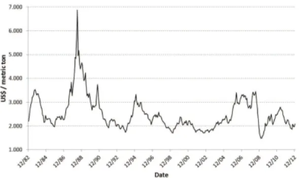
In order to define and calibrate the stochastic behavior of aluminum prices, historical prices in US$/metric ton from December 1982 to April 2013 (monthly basis) were used. This series was adjusted for US inflation rate using Consumer Price Index – CPI obtained from Bloomberg at April 2013 prices. Figure 1 shows the historical behavior of aluminum prices in April 2013 US$/Ton.
In order to verify the adequacy of a MRM for this series an Augmented Dickey-Fuller (ADF) test was run on the log of the series to verify its stationarity and the resulting t-statistic was –2.7570. Although this value rejects the presence of a unit root (therefore rejecting the adequacy of a Geometric Brownian Motion) at a 10% level (–2.5710), it does not reject it at a 5% level (–2.8694). Therefore a Variance Ratio test was also applied to the series, as suggested by Pindyck (1999). The result can be observed in Figure 2.
Although it increases initially, the Variance Ratio quickly drops below 1 as the time lag increases and
Figure 1. Monthly aluminum prices in 04/2013 in US$. Source:
London Metal Exchange. https://www.lme.com/metals/reports/ averages/.
Figure 2. Variance ratio test on aluminum log prices.
series suggest that electric energy prices long term mean appears to be closer to the lower level of PLD scenarios and jumps occur only upwards. We model the jump size as a triangular distribution with a minimum of US$ 100/MWH, mean of US$ 150/ MWh and maximum of US$ 200/MWh. These values are obtained by filtering all series of PLD simulation
3.4.
Stochastic modeling of energy prices
We use the PLD (Settlement Price Difference) to model energy prices in the Brazilian unregulated market, which is the price used for energy sales in the short term market. PLD prices are determined by considering the equilibrium between the benefits of future use and storage of water in the reservoirs and the cost of immediate generation through the dispatch of thermal plants in order to optimize the integrated grid system in Brazil. This is done with the use of computational models that estimate a Marginal Cost of Operation (CMO) by an optimization method equivalent to Lagrange’s multiplier associated to a demand restriction. The trade-off in this market consists in the choice of the best time for hydro or thermal generation. This is due to the fact that an excessive use of hydro power today might imply in a high future cost of thermal generation if there is low rainfall in the future. On the other hand, if water is saved and rainfall inflows are high in the future, a spillover of the reservoirs may be necessary representing wastage of energy and increase in operational costs. Historical values for PLD for most representative sub-market (South East-Center West: SECO) are shown in Figure 5.
Again we verify the adequacy of a MRM for this series using an ADF test. The t-statistic returned was –5.0477, which rejects the unit root at a 1% level (–3.4475), strongly confirming a mean reversion behavior. Although, the historic PLD series shown in Figure 5 suggest the presence of jumps along with a mean reversion behavior, it nevertheless does not allow a robust calibration of the jump behavior process since very few jump events can be observed in the 12 year period (2001/6, 2007/8 and 2012/3). PLD price simulation is done with a complex computational system called NEWAVE that calculates the optimum price policy based on current and future costs and takes into account a planning horizon of five years. The simulated prices present a stochastic behavior suggesting the presence of jumps, as can be observed in Figure 6.
In order to determine the jump parameters of the energy price diffusion process we use two thousand simulations of PLD from the NEWAVE system from January 2013 to September 2017, with a few simplifying assumptions. To determine the frequency of the jumps, we established an arbitrary threshold of US$125/Mwah above which the price is assumed to be a jump. This provided a frequency of 5.27% for each month of simulation.
Differently from the approach used by Dias
& Rocha (1999) for oil prices where direction of the jumps is also random, observation of the PLD
Figure 4. Aluminum price scenarios (250).
Table 1. MRM parameters for aluminum prices.
Mean Reversion Parameters for Aluminum Prices
Parameter Value
Aluminum Initial Price 1,861.02 (US$/ton)
Long term mean SA 2,513.16 (US$/ton)
Volatility per year - sA 20.39 (%)
Mean Reversion Speed per year - ηA 0.332
Normalized risk premium – π/η 0.0450 (%) Risk Adjusted Long term mean - S*
A 2,304.65 (US$/ton)
Figure 5. Historical PDL for SE-CO sub market.
sales contracts have been fulfilled through the acquisition of scrap aluminum in the metal market.
We assume that the default operating mode
q1 of the smelter is the production of aluminum,
and that the alternate mode q2 is the suspension of
aluminum production and sales of electric energy. In addition, the firm incurs in a switching cost λ12 every time it changes from operating mode q1 to q2,
and an asymmetric switching cost λ21 every time it changes back from q2 to q1. If operating in mode q1
(aluminum production), and the expected cash flows for the next period in mode q1 are still greater than
the mode q2 expected cash flows (energy sales) plus
the switching costs λ12, then the firm will maintain the current operating mode q1. On the other hand
if the expected cash flows from mode q2, including
the switching cost λ21, are greater, then the firm will switch modes from q1 to q2. Thus in this situation
(mode q1) the optimal operation mode decision for
nest period is given by: qt+1 = max{q1 t+1; q
2
t+1 – λ12}.
Similarly if the firm is already operating in mode q2 (energy sale), the next period mode will
be determined by the comparison of that period cash flow: qt+1 = max{q2
t+1; q
1
t+1 – λ21}, whichever
is higher.
3.6.
Model assumptions
We model a typical aluminum smelter plant in Brazil based on market parameters and industry above US$ 125/MWh, and fitting these values with a
symmetrical triangular distribution after rounding to integer values. Table 2 summarizes the assumptions and values used for the jump model of PLD.
In order to calibrate the Mean Reversion component of the PLD, the historical series of PLD price was used with a barrier at U$S 125/MWh in order to filter for the jumps effect. Also only values after April 15, 2005 were used, when the series began to behave in a more random or stochastic way, without long periods of fixed minimum values, as can be observer in Figure 4. These series and all parameters where converted to a monthly base.
Using the same approach as with aluminum prices, the parameters shown in Table 3 were obtained. The simulation process of PLD values are restricted to a range between US$ 8.16/Mwh and US$ 316.69/MWh, since these are the minimum and maximum values accepted by the Regulatory Agency (ANEEL) for the time sample studied. These prices are issued in Brazilian R$ and converted to US$ at the prevailing rate of 2.00 R$/US$ of time of the study.
The risk premium of the process for the PLD was obtained through numerical methods in order to discount the projects cash flows at the risk free rate. It was still necessary to compensate the long term mean of the MRM process for the added jumps which are only positive in this study in order to have a process that will return the same value of the deterministic process in a simulation analysis. This was done using a numerical approach and the risk neutral and compensated long term mean S**
E
to be used in Monte Carlo simulations is also listed in Table 3.
3.5.
Application to an aluminum smelter
In an aluminum smelter, alumina (aluminum oxide) is transformed into metal aluminum through an electrolytic reduction process. The main operating cost is the price of the electricity needed for the reduction reaction. Therefore there is an opportunity to maximize the smelter´s cash flows by taking into account the volatilities of aluminum and energy prices and the managerial flexibilities embedded in the operation of the plant.
One possibility available to the smelter in times of high energy prices is to temporarily suspend the alumina reduction process and sell the energy already contracted through long term contracts or from co-generation. In regions where the cost of energy is relatively high, aluminum producing plants have opted to close smelters and or move to regions with greater supply and lower costs of energy. In the case of temporary suspension, pre-established aluminum
Table 2. Assumptions – jump parameters.
Jump parameters for the MRM with Jumps model for PLD
Parameter Value
Price Level above which is considered
Jump 125.00 (US$/MWh)
Frequency of Jumps per time period 5.27 (%/semester) Size of Jumps triangular
distribution - minimum 100.00 (US$/MWh)
Size of Jumps triangular
distribution - medium 150.00 (US$/MWh)
Size of Jumps triangular
distribution - maximum 200.00 (US$/MWh)
Table 3. MRM parameters for energy prices – PLD.
Mean Reversion Parameters for PLD
Parameter Value
Initial value * 109.97 (US$/MWh)
Long Term Mean of Energy - SE 77.605 (US$/MWh)
Standard Deviation of Energy - sE 127.82 (% /year)
Mean Reversion Speed of Energy - ηE 1.007 (per year)
Normalized Risk Premium - PLD 0.0269
Risk Neutral Long Term Mean PLD - S*
E 72.16 (US$/MWh)
Risk Neutral Long Term Mean compensated for positive jumps - S**
E
57.61 (US$/MWh)
possibly retrain its workforce at an estimated cost of $1 million dollars. In addition, the useful life and reactivation cost of the electrolytic furnaces depend on the length of time the interruption lasted. For short production interruption periods each furnace can be reactivated at an estimated cost of $10,000 dollars, but this implies in a loss of 30% of its useful life. In case of a longer interruption time, it is necessary to change the lining at a cost of $100,000 per furnace. Considering the different time usage of the furnaces, we assume that 30% of the furnaces will have their linings reused. Therefore, for a plant with 500 smelting furnaces, production restart cost assuming that all furnaces are idle will imply in a cost of: 500 x (70% x US$ 100,000 + 30% x US$ 10,000) = US$ 37.5 million dollars.
3.7.
Model structure
The cash flow model of the smelter considers the cash flows of each of the operation modes and incorporates the uncertainties of both stochastic processes of energy and aluminum prices, while the temporary suspension option exercise also considers the asymmetric costs of mode change. The cash flow of operation mode q1 considers the production
of metallic aluminum through catalytic reduction for commercialization. Costs involved are those of alumina consumption, energy usage and other data available from public sources. Tables 4 and 5
represent the main assumptions adopted for the model. We also assume that plant productivity is constant over the life of the unit through continuous capital expenditure reinvestments.
The cost of pre-contracted energy was assumed to be US$ 34/MWh considering the average sales contracts from a distribution company. For simplification we also assume that this is also the opportunity cost equivalent of energy from a self-sufficient smelter from co-generation. This price level is equivalent to the average of long term contracts in Brazil, and must not be confused with the short term spot energy price (PLD), with is much more volatile and not applicable to large supply contracts, such as a smelter.
Switching costs derive from the following: Switching costs λ12:
As the change from the default mode q1 to q2
implies shutting down the reduction units, these costs involve the layoff or relocation of the working force. This cost is estimated at US$ 2 million and also brings about a decrease in other production costs to US$440/t, (from US$ 640/t when in mode q1), aside
from the costs related to alumina consumption. Switching costs λ21:
Involves the cost of changing back from mode
q2 to q1. Once the firm suspends operations, in order
to reactivate the reduction units it must rehire and
Table 4. Assumptions for operation mode q1 – Aluminum production.
Assumptions Quantity / Values
Installed capacity 500,000 (tons per year of metallic aluminum)
Operation Plant Lifetime 20 (years)
Reduction units 500 (units)
Energy consumption 15.88 (MWh/ton of aluminum produced)
Pre-contracted energy cost 34 (US$/MWh)
Alumina cost 14.5 (% of aluminum price at LME + 37 US$/ton)
Alumina consumption 1.92 (tons alumina per ton of aluminum)
Aluminum price (US$) Stochastic variable based on LME indicators.
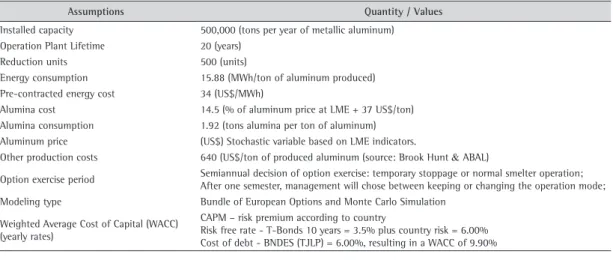
Other production costs 640 (US$/ton of produced aluminum (source: Brook Hunt & ABAL)
Option exercise period Semiannual decision of option exercise: temporary stoppage or normal smelter operation;After one semester, management will chose between keeping or changing the operation mode;
Modeling type Bundle of European Options and Monte Carlo Simulation
Weighted Average Cost of Capital (WACC) (yearly rates)
CAPM – risk premium according to country
Risk free rate - T-Bonds 10 years = 3.5% plus country risk = 6.00% Cost of debt - BNDES (TJLP) = 6.00%, resulting in a WACC of 9.90%
Table 5. Assumptions for operation mode q2 – energy sales.
Assumptions Quantity/ Values
Contracted energy consumption 15.88 (MWh/ton of installed capacity)
Pre-contracted energy cost 34 (US$/MWh)
Energy spot price (US$) Stochastic variable based PLD price.
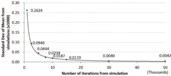
thousand for each of the sensitivity analysis values using the risk neutral approach. Such number of iterations is sufficient for the required precision, as can be observed in Figure 8.
The decision to switch operating modes is taken considering the maximization of cash flows together with the switching costs. This decision is based on the prices available to management at the moment of the decision and we assume the firm can immediately enter into a six month (one period) contract at those prices. Therefore this decision is based on the assumption that the firm can sell for the next six months a contract based on the values prices available at this moment. This approach is similar to that adopted in studies such as Bastian-Pinto et al. (2010) where the decision coincides with the realization of prices of the uncertain variables. Figure 9 and 10 illustrates a single realization of the simulation showing the switch of operation mode through maximization of cash flows and considering conversion costs.
The value of the aluminum smelter with the option to switch operating modes under price uncertainty and asymmetric switching costs as described increases to US$ 2,079.7 million, an increase of 48.8% over the base case q1. The
simulation indicates that the plant, in average, remains in temporary suspension mode q2 35.55%
of the time, which is significantly higher than the 5.27% jump frequency of energy prices. This may operation costs. Cash flow of operation mode q2
on the other hand, comes exclusively from selling at PLD price the pre-contracted (or co-generated) available energy. Once the operation mode that maximizes cash flow is determined, the algorithm values if the option to switch is still advantageous when considering the switch costs. If not, the smelter continues to operate in the current mode.
The value of the temporary suspension of the smelter is estimated by calculating the present value of semiannual cash flows for 20 years of operation for each case considering the future price uncertainties of aluminum and energy under the risk neutral measure and no residual value. A third hybrid mode is also considered, in which aluminum production is set a level of 80% of the installed capacity and 20% of the energy is available for commercialization. In this mode, q3, there are no reduction in fixed costs,
but only 80% of the alumina of q1 is used. There
are also no costs of switching between q1 and q3 or
back, since the operation level of the plant decreases but is not shut down.
The base case values for each of the three modes provide the following deterministic Present Values (PV) considering a WACC of 9.90% per year:
q1 = US$ 1,397 million, q2 = US$ 1,010 million and
q3 = US$ 1,203 million. These base case values will
be used as comparison with the results of the Real Options valuation.
The cash flows corresponding to the deterministic valuation in each period are shown in Figure 7, where we also show possible switches between the three available modes. We arbitrarily assume the firm starts in mode q3. Given that initial energy prices, at
the time of this study, are high (approximately US$ 180/Mwh) and that aluminum prices are relatively low, the firm will immediately switch to energy sales mode q2 in the next period. As expected cash flow
revert to their mean value, it becomes increasingly profitable for the firm to switch to mode q1 (100%
aluminum production), but this will not occur immediately due to the high conversion costs λ21. Only when the difference is greater than the cost to switch will the firm exercise this option. It is also worth noting that from a deterministic analysis q3
will never be the mode of choice as its long term cash flows are lower than that of q1.
4. Results
The model was run using Monte Carlo Simulation with @Risk software from Palisade Decision Tools. Fifty thousand iterations were performed to determine the value of the switch options and twenty
Figure 7. Deterministic cash flows for the different possible
operation modes.
Figure 8. Sensitivity of the standard deviation of results to
1,672 million, an increase of 19.73% above the base case. This mode is chosen 25.4% of the time. If we assume that there are no switching costs at all, the value of the plant increases to US$ 2,204 million, or 57.81% above the base case, and a frequency of full stoppage is 32.13%. In this case in 9.7% of semesters mode q3 will be the optimal choice. As expected, the
switching costs influence the results, but this effect is not as significant as one would expect.
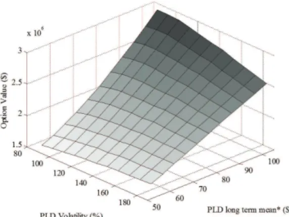
As usual, the results depend on the parameters used in the model. A sensitivity analysis on the most relevant ones was done in order to check their significance and impact on the smelter value with the option. We analyze the long term mean of PLD energy prices SE and the PLD energy volatility sE.
Results are shown in Figure 11. In the z axis: option value, refers to the total value of the smelter, with the switch option. As can be observed, the change of parameters of energy prices do influence option value, but, PLD volatility (sE) is less influent than the long term mean (SE) to which PLD reverts. It is also interesting to note that for low values of SE, a rise in volatility (sE) brings higher value of the option, whereas for high values of SE, the opposite happens: greater volatility diminishes the option value. This is due to the high mean reversion speed factor ηE which counters the effect of volatility on the price, and at high values of equilibrium level, has this effect amplified.
5. Conclusions
We developed a switching option model with asymmetric switching costs and multiple uncertainties and apply the results to the case of an aluminum smelter which has the option to change operating strategies as uncertainty over aluminum and energy prices are resolved. The aluminum and energy price uncertainties are modeled as mean reverting diffusion process with jumps, and the switch options are modeled as a bundle of European options over the life of the aluminum plant. The model is then solved by means of a Monte Carlo simulation under the real options approach.
The results indicate that a significant portion of the value of the plant can be derived from the flexibility to partially or totally suspend production of aluminum in favor of selling energy in the market. The results also show that traditional valuation methods are unable to capture the value of the economic gains derived from this flexibility, which has option like characteristics and thus must be valued under option pricing methods. This result can be generalized for other electro-intensive industries that indicate that the high conversion cost λ21 might
inhibit the switch back to q1, keeping the operation
“stuck” in mode q2 until the difference in cash flows
is large enough to compensate conversion costs. This behavior can be observed in Figure 9 in semesters 5, 12, 13 and 15, and in Figure 10, in semesters 2, 7, 22, 25 and 35. Also on 8.7% of periods the firm operates in mode q3.
If only modes q1 and q3 are considered, there are
no switching costs and the value of the plant is US$
Figure 9. Single realization sample of cash flow trajectories.
Figure 10. Single realization sample of cash flow trajectories.
Figure 11. Sensitivity of option value to volatility and long
Political Economy, 81(3), 637-654. http://dx.doi. org/10.1086/260062
Brennan, M. J., & Schwartz, E. S. (1985). Evaluating natural resource investments. Journal of Business, 58(2), 135-157. http://dx.doi.org/10.1086/296288
Byko, M. (2002). TMS plenery symposium: energy reduction in the aluminum industry. Journal of Minerals, Metals and Materials Society, 54(5), 39-40. http://dx.doi. org/10.1007/BF02701695
Das, S., Long III, W. J., Hayden, H. W., Green, J. A. S., & Hunt Jr., W. H. (2004). Energy implications of the changing world of aluminum metal supply. JOM, 56(8), 14-17. http://dx.doi.org/10.1007/s11837-004-0175-6
Dias, M. A. G., & Rocha, K. (1999). Petroleum concessions with extendible options using mean reversion with jumps to model oil prices. In 3rd Annual International Conference on Real Options, Leiden, Netherlands. Dixit, A., & Pindyck, R. (1994). Investment under uncertainty.
Princeton: Princeton University Press.
Dockendorf, J., & Paxson, D. (2013). Continuous rainbow options on commodity outputs: what is the real value of switching facilities? The European Journal of Finance, 19(7-8), 645-673. http://dx.doi.org/10.1080/1 351847X.2011.601663
Fontoura, C. F., Brandão, L. E., & Gomes, L. L. (2014, in press). Elephant grass biorefineries: towards a cleaner Brazilian energy matrix? Journal of Cleaner Production. Kulatilaka, N. (1993). The value of flexibility: the case
of a dual-fuel industrial steam boiler. Financial Management, 22(3), 271-280. http://dx.doi. org/10.2307/3665944
Merton, R. C. (1973). Theory of rational option pricing. The Bell Journal of Economics and Management Science, 4(1), 141-183. http://dx.doi. org/10.2307/3003143
Morck, R., Schwartz, E., & Stangeland, D. (1989). The valuation of forestry resources under stochastic prices and inventories. Journal of Financial and Quantitative Analysis, 24(4), 473-487. http://dx.doi. org/10.2307/2330980
Ozorio, L., Bastian-Pinto, C. L., Baidya, T. K. N., & Brandão, L. E. T. (2013). Investment decision in integrated steel plants under uncertainty. International Review of Financial Analysis, 27, 55-64. http://dx.doi. org/10.1016/j.irfa.2012.06.003
Paddock, J. L., Siegel, D. R., & Smith, J. L. (1988). Option valuation of claims on real assets: the case of offshore petroleum leases. Quarterly Journal of Economics, 103(3), 479-508. http://dx.doi. org/10.2307/1885541
Pindyck, R. S. (1999). The long-run evolution of energy prices. Energy Journal, 20(2), 1-27. http://dx.doi.org/10.5547/ ISSN0195-6574-EJ-Vol20-No2-1
Schwartz, E. S. (1997). The stochastic behavior of commodity prices: implications for valuation and hedging. Journal of Finance, 52(3), 923-973. http://dx.doi. org/10.1111/j.1540-6261.1997.tb02721.x
Siegel, D. R., Smith, J. L., & Paddock, J. L. (1987). Valuing offshore oil properties with option pricing models. Midland Corporate Finance Journal, 5, 22-30.
Slade, M. (2001). Valuing managerial flexibility: an application of real-option theory to mining investments. Journal of
possess this same flexibility, and which can benefit from optimally shutting down production in times of high energy prices.
For policy makers, these findings indicate that electricity price signals can affect both supply and demand for electricity, as flexible electro-intensive industries can switch from being consumers to suppliers of electricity in times of energy shortages, as was the case in early 2014 in Brazil, reducing the need for widespread energy rationing. This “soft” form of rationing may be preferable to “hard” mandatory across the board electricity cuts.
As for the limitations of this paper, the energy price model adopted is only applicable to the hydro based Brazilian electrical energy market, and we have shown that the model is sensitive to the parameters of the stochastic processes adopted. The PLD settlement prices are also actual not market prices, as they are defined unilaterally by the CCEE clearing chamber. Suggestions for further research include advances in calibration and parameter determination that could help provide more precise results, as well as the study of the interaction between variables over time and how this may impact the decisions of the firm. For simplification purposes we also considered that prices for the next immediate semester period at the time of the decision of whether to suspend or operate the plant are fixed and equal to the current stochastic price at the beginning of the period. A different approach could also be adopted by considering that all future prices are uncertain, which would change the nature of the managerial flexibilities embedded into the plant from European to American options.
References
Adkins, R., & Paxson, D. (2012). Real input-output energy-switching options. The Journal of Energy Markets, 5(3), 3-22.
Bastian-Pinto, C., Brandão, L., & Alves, M. L. (2010). Valuing the switching flexibility of the ethanol-gas flex fuel car. Annals of Operations Research, 176(1), 333-348. http:// dx.doi.org/10.1007/s10479-009-0514-7
Bastian-Pinto, C., Brandão, L., & Hahn, W. J. (2009). Flexibility as a source of value in the production of alternative fuels: The ethanol case. Energy Economics, 31(3), 411-422. http://dx.doi.org/10.1016/j.eneco.2009.02.004 Berger, M. C. (1988). Predicted future earnings and
choice of College Major. Industrial and Labor Relations Review, 41(3), 418-429. http://dx.doi. org/10.2307/2523907
Bessembinder, H., Coughenour, J. F., Seguin, P. J., &
Smoller, M. M. (1995). Mean reversion in equilibrium asset prices: evidence from futures term structure. Journal of Finance, 50(1), 361-375. http://dx.doi. org/10.1111/j.1540-6261.1995.tb05178.x
Acknowledgements
The authors thank CNPq for the financial support through the Edital Universal grant, as well as FAPERJ through the APQ1 grant.
Environmental Economics and Management, 41(2), 193-233. http://dx.doi.org/10.1006/jeem.2000.1139 Trigeorgis, L. (1990). A real options application in natural
resource investments. Advances in Futures and Options Research, 4, 153-164.