RBRH, Porto Alegre, v. 22, e16, 2017 Scientiic/Technical Article
http://dx.doi.org/10.1590/2318-0331.011716048
Modeling metabolism in an integrated subtropical watershed-reservoir system
Simulação do metabolismo em um reservatório subtropical integrado à bacia hidrográfica
Vinicius Teixeira Tambara1, Carlos Ruberto Fragoso Júnior2 and David da Motta Marques3
1Universidade Federal do Rio Grande do Sul, Porto Alegre, RS, Brasil 2Universidade Federal de Alagoas, Maceió, AL, Brasil 3Universidade Federal do Rio Grande do Sul, Porto Alegre, RS, Brasil
E-mails: [email protected] (VTT), [email protected] (CRFJ), [email protected] (DMM)
Received: April 18, 2016 - Revised: October 16, 2016 - Accepted: November 07, 2016
ABSTRACT
Reservoirs are considered transition systems between rivers and lakes with particular features due to its morphology and watershed
inlows. Studies about aquatic metabolism in subtropical aquatic ecosystems, particularly in reservoirs, have been based on direct measurements and statistical relationships in speciic gauge stations of the system rather than on analytical models, which are capable
of representing the metabolic processes at different temporal and spatial scales. This paper aimed to evaluate the temporal variability of metabolism in a subtropical reservoir, named Faxinal reservoir, located in Caxias do Sul, Rio Grande do Sul state, Brazil, by using an
ecological model (IPH-ECO) which was coupled with a hydrological model (IPH-II) to estimate inlows and nutrient loadings from the
watershed. After model calibration, metabolic daily rates of gross primary production (GPP) and respiration (R) were estimated over a 1-year period (from November 2011 to December 2012), considering a process-based algorithm based on dissolved-oxygen budget implemented in the IPH-ECO model. Faxinal reservoir were net heterotrophic 97% of the simulation period. The temporal variability of GPP and R followed the general pattern of phytoplankton biomass in reservoir, which was more related to autochthonous factors such as water residence time, light availability, nutrient concentration and zooplankton grazing. Only during heavy rainfall period, increasing the terrestrial exports, the concentration of phosphorus was higher leading to an increase of chlorophyll-a concentration
and hence metabolic rates of GPP and R. Therefore, considering the long dry period during the simulation, the aquatic metabolism of Faxinal reservoir is more inluenced by the internal dynamic of the aquatic ecosystem than the watershed inputs.
Keywords: Ecological modeling; Metabolism; Reservoir.
RESUMO
A morfologia e o aporte da bacia hidrográica fazem dos reservatórios um sistema de transição entre rios e lagos com características particulares em termos hidrodinâmicos e de metabolismo. Estudos sobre o metabolismo em ecossistemas aquáticos subtropicais, particularmente em reservatórios, têm se baseado mais em medições diretas e pontuais e em relações estatísticas que em modelos analíticos capazes de representar os processos envolvidos em diferentes escalas espaço-temporais. O objetivo deste trabalho foi avaliar
a variabilidade temporal do metabolismo de um reservatório subtropical na cidade de Caxias do Sul/RS através do modelo ecológico
IPH-ECO, o qual foi acoplado ao modelo hidrológico IPH-II para estimar as contribuições da bacia hidrográica. Após a calibração dos modelos, foram calculadas as taxas metabólicas de produção primária (GPP) e respiração (R) para o período de nov/2011 a dez/2012 através dos processos que compõem o balanço de oxigênio no modelo IPH-ECO. O reservatório apresentou um metabolismo autotróico em 97% do período de simulação. As variações temporais de GPP e R acompanharam o padrão de variação da comunidade itoplanctônica, sendo esta variação mais associada a fatores autóctones, tais como tempo de residência, disponibilidade de luz na água, concentração de nutrientes e predação por herbívoros. No período de chuva, foi observado um maior aporte de fósforo da bacia hidrográica que provocou um aumento da concentração de cloroila-a e, consequentemente, das taxas de GPP e R. Considerando o período simulado, o metabolismo do reservatório respondeu mais em função da dinâmica interna do sistema do que ao aporte da bacia hidrográica.
INTRODUCTION
Inland freshwater ecosystems are known as metabolically-active compartments regulating the cycling of organic matter and nutrients, sediment storage and production and consumption of greenhouse gases such as carbon dioxide and methane (RAYMOND et al., 2013). Metabolism of aquatic ecosystems can be deined as the study of ecosystem structure and functioning under three main aspects: production, consumption and decomposition of organic matter (CARMOUZE, 1994). Therefore, the analysis of aquatic metabolism allows researchers to make inferences about the effects of upland loadings and environmental changes due to anthropic
activities (e.g. change of land use, irrigation and ishing) and climate
conditions such as air temperature, wind speed and precipitation (KOSTEN et al., 2010; ZHANG et al., 2012) on the water quality
and quantity of aquatic ecosystems.
Aquatic metabolism can be determined through biological
balance between two processes: production of organic carbon and oxygen, represented by gross primary production (GPP), and consumption of organic carbon and release of carbon dioxide by respiration (R). This balance is represented by the net ecosystem production (NEP=GPP-R) which indicates whether reservoir is a net autotrophic (GPP>R or NEP>0) or heterotrophic (R>GPP or NEP<0) ecosystem (COLE et al., 2000). The metabolic rates of GPP, R and NEP may vary at different time and spatial scales according to physical, chemical and biological conditions of the ecosystem and its interaction with adjacent watersheds (HANSON et al., 2006).
Respiration in younger reservoirs, less than 10 years, is
mainly inluenced by the amount of looded labile organic matter
(KIM et al., 2012; BARROS et al., 2011). On the other hand, recent studies indicated that bacterial respiration in older lakes and reservoirs is more associated with inputs of dissolved organic carbon (DOC) and dissolved inorganic carbon (DIC) from the catchment (SOBEK et al., 2006; SOLOMON et al., 2013) which enhance net heterotrophic ecosystem metabolism. Moreover, agricultural and urban catchments might contribute greatly to the increase of external nutrient loadings that can be higher during storm events due to erosion and runoff, intensifying either net autotrophic or heterotrophic metabolism (MAROTTA et al., 2010).
Other important features, which, by the way, affect considerably the metabolism of deep reservoirs, are thermal
stratiication and water mixing regime inluencing distribution
of nutrients, organisms and oxygen through water column (HODGES et al., 2000; EVANS et al., 2008; PANNARD et al., 2011). Furthermore, the operation of reservoir combined to the hydrological variability of the basin may affect reservoir residence time. This hydromorphological variable indicates the amount of
time water stays in a reservoir or lake, which may directly inluence
the dynamic of microorganisms such as phytoplankton and hence contributing to autotrophic metabolism.
Estimates of metabolism in terms of GPP, R and NEP
in aquatic ecosystems can be determined either by lumped
models based on “free-water” changes in dissolved oxygen (DO) concentrations (ODUM, 1956) or by distributed process-based models (ANTENUCCI et al., 2012; CAVALCANTI, 2013).
The “Free Water” technique assumes that changes in diel oxygen concentration relect the biological balance between photosynthetic
production and respiratory consumption as well as the physical
exchange of oxygen between air and water. This technique estimates
GPP and R by measuring temporal changes in DO concentration
through gauge stations using high-frequency sondes at speciic points in the aquatic system, and has been applied in a variety of
ecosystems (HANSON et al., 2003; VAN DE BOGERT et al., 2007; COLOSO et al., 2011; STAEHR et al., 2010). However, this method has limitations and assumptions in representing the ecosystem physical and ecological heterogeneity, as well as the whole-lake metabolism. In this sense, ecological modeling shows as a valuable tool in order to represent the non-linear variability of dissolved oxygen (DO) and integrate metabolic, physical and chemical processes involved in the production and consumption
of DO at more reined temporal and spatial scales, allowing the
formulation of hypotheses about ecosystem dynamics.
Among some process-based ecological models, the water
quality models coupled to hydrodynamic models have shown an
outstanding potential for their applications (3D CWR-ELCOM - HODGES et al., 2000; DYRESM - GAL et al., 2002). This linkage between biogeochemical and hydrodynamic processes of the
ecosystem enables the lexible and integrated representation of
DO with water level variation, trophic interactions and nutrient/gas cycling (FRAGOSO JÚNIOR; FERREIRA; MARQUES, 2009; TESTA et al., 2014). In addition, it is possible to include hydrological
variables into the modeling, such as inlow from tributaries
and nutrient loads from shorelines and watersheds, by using ecological models coupled with hydrological models (Multi-level Watershed-Reservoir Modeling System-MWRMS - ZHANG et al., 2012). Nevertheless, modeling the metabolism dynamics in subtropical reservoirs linked to its watershed is still incipient. Therefore, this work aims to evaluate the temporal variability of metabolic rates by applying the process-based model IPH-ECO (FRAGOSO JÚNIOR et al., 2010) as well as the responses of the
Faxinal reservoir to different inlows from the watershed, which
was simulated by the hydrological model IPH-II (BRAVO et al., 2007). The analysis of the temporal variation of metabolism in Faxinal reservoir through the simulation of biogeochemical and hydrodynamic processes lead to the answers for the following
questions: (a) Is there any relationship between the metabolism of the reservoir and its watershed in terms of inlows and nutrient
loads?; (b) What are the abiotic and biotic variables (temperature,
chlorophyll-a, nutrients) which have the most inluence on the
reservoir metabolism?
MATERIALS AND METHODS
Study area
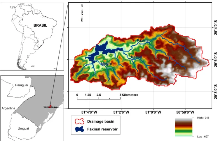
The Faxinal reservoir (29°05’00” S; 51°03’30” W) is the main water supply system of the city of Caxias do Sul in southern Brazil (supply 64% of the total population of 400.000 habitants).
Faxinal is a deep (maximum depth of 24 m), warm monomictic and eutrophic reservoir (total phosphorus concentration of 29.4 µg/L and chlorophyll-a of 15 µg/L, epilimnion annual mean) showing a low variation in the water level over the year, around 1.50 m.
Thermal stratiication of reservoir water column occurs during
summer and spring periods (January-May and September-December) whereas in winter water mixing regime takes place. The regional climate is subtropical without a dry season (Cfa type; KÖPPEN, 1936) with an average annual temperature of 16 °C and precipitation between 1.800 and 2.200 mm (BECKER et al., 2008).
Sampling and ield measurements
The limnological variables considered in the model calibration were measured monthly during 13 campaigns carried out by Souza (2013) from November/2011 to December/2012. Samples were collected at 6 stations through the reservoir surface (Figure 2). The vertical proiles of water temperature, dissolved
oxygen, PH and conductivity were determined in the ield by
using the YSI 6000 multiparameter data sonde. The sonde data were gathered at all 6 stations for each 1 meter depth from the bottom to the surface of the reservoir. Water transparency was estimated with Secchi disc. Surface samples (from 0 to 0.5 m) were gathered by using “Van Dorn” bottle type, then they were refrigerated for transportation and submitted to lab analysis of
inorganic nutrients, organic and inorganic carbon (TOC, DOC, DIC), alkalinity, chlorophyll-a, phytoplankton and zooplankton biomass.
IPH-ECO model description
IPH-ECO is an ecological complex dynamic model for
inland aquatic ecosystems such as lakes, reservoirs and estuaries
(FRAGOSO JÚNIOR; FERREIRA; MARQUES, 2009; IPH-ECO Figure 1. Map of the Faxinal Reservoir (3.1 km2) showing its drainage basin.
Scientiic Manual). The model can be used in three-dimensional (3D)
applications and also in 0D, 1D or 2D for simple approaches. Basically, the model consists of two modules: (a) a detailed hydrodynamic
module, describing quantitative lows and water level (CASULLI, 1990; CHENG et al., 1993); and (b) a water quality module which
deals with nutrient transport mechanisms and the whole aquatic
food-web interactions (e.g. phytoplankton, macrophytes, zooplankton,
benthos and ishes), being able to represent the entire cycle of
nutrients (e.g. Phosphorus, nitrogen, silica) and dissolved oxygen. Water temperature is calculated through an energy balance between
heat luxes on the water surface. In this work, a 0D IPH-ECO model
was implemented to determine the reservoir volume and water level
through a water balance and water quality variables through a mass
balance between biogeochemical processes.
IPH-ECO simulates metabolism through the “Free Water”
technique (ODUM, 1956) which uses the governing equation for estimating free-water metabolism from measurements of dissolved oxygen:
2 O
GPP R F A t
∂ = − + +
∂ (1)
In the model, each term of the equation above is broken
down into the processes referring to production and/or consumption
of dissolved oxygen as shown by the equation below:
2
2 2 2 2
2 2 3
Pr ( Re
Re ) Re
O
wO odPhyt wO MinDetW wO NitrW wO spPhyt t
wD spZoo wO aer wO UptNO Phyt
∂ = − + +
∂
+ + + (2)
GPP is composed of algal production of phytoplankton (wO2 Pr odPhyt), R is composed of mineralization processes (wO2MinDetW), bacterial nitriication (wO2NitrW), algal respiration (wO2RespPhyt) and zooplankton (wD RE spZoo), F represents the reaeration process (wO2 Re aer) and A represents non-biological process like algae assimilation of nitrate (wO2UptNO3Phyt).
The reaeration lux can be determined by the equation below:
( º 20)
2Re Re * ( 2 2 ) *1.06T C
wO aer k=− aer O Sat O Água − (3)
The reaeration constant kReaer is a function of wind speed
(Vwind) deined by the empirical equation below:
0,5 2
Re 0.727 * 0.371* 0.0376 *
k aer= Vwind − Vwind+ Vwind (4)
Input variables and boundary conditions
Input data for the model included daily records of evaporation and precipitation and hourly records of air temperature, wind speed and direction, solar radiation and relative humidity obtained from two meteorological stations of INMET (National Institute of Meteorology) located near the reservoir but outside of its drainage basin. For model simulations, it was considered an hourly time-step.
The boundaries of the Faxinal Basin were delimited by using satellite images in raster format obtained from Shuttle Radar Topography Mission (SRTM) with a 90m resolution. The land occupation type in the Faxinal basins was determined through
the visual classiication of 2010-LANDSAT 5 satellite images
considering four major land occupation types in the basin: crop and pasture, forest, water and urban (Figure 3).
The Faxinal basin is mostly rural presenting a cluster of small urban areas scattered in a crop-growing area. For a more detailed analysis, the Faxinal basin was divided into seven sub-basins. The composition of the different land uses in each sub-basin was similar and is as follows: 3.3% of water; 9.1% of urban area; 60.5% of forest and 27% of crop and pasture. SB-1 has the largest area of crop and pasture that corresponds to around 39% of its total area. According to a study carried out in the Faxinal basin SB-2 and SB-4 have the largest crop area, around 12% and 14%, whereas in SB-7 it is located part of Ana Rech urban district where a waste treatment plant is currently operating (VARGAS et al., 2013).
The rainfall-runoff hydrological model IPH-II (BRAVO et al., 2007; Manual de Conceitos WIN_IPH2) simulated the reservoir
inlows from the seven sub-basins. Hourly precipitation and
evaporation were used as inputs for the model. Also, an hourly time step was adopted for the simulations enabling a better description of the sub-basin hydrographs, since the areas are
quite small (1.5 to 29.4 km2) and their time of concentration are less than 2 hours.
Iniltration parameters of the equations that describe the separation of overland and groundwater lows (I0 and h which
deine maximum humidity capacity of soil and Ib, the maximum
iniltration capacity) were based on the land use type in the seven sub-basins. The lag time of overland low Ks and the time of concentration tc were obtained through relations that take into account watershed topographic characteristics as proposed by Germano et al. (1998).
A preliminary estimate of orthophosphate, ammonium and nitrate loads were made based on the hydrochemical monitoring conducted by SAMAE (Sanitation Company of Caxias do Sul) technical team at the 7 sub-basins outlets over the period of april/2012-april/2013. During the months without monitoring, nutrient loads were estimated through the calibration of the model biogeochemical component (referred to phosphorus and nitrogen) simulated in the model, which, besides taking account
the abiotic variables, consider the effects of loads and lows
from watershed on nutrient cycling. Daily nutrient loads were calculated by interpolating the monthly load values. Despite the high variability of monthly nutrient loads in the Faxinal reservoir, only the nutrient load peaks had a major effect on the simulated concentration of nutrients, which were more sensitive to the internal abiotic process in the reservoir.
Model calibration
In this study, the calibration process involved models with different time-spatial scales and various inputs and outputs. Due to this interaction between the models, the calibration of IPH-ECO
was performed in a stepwise scheme: irst, the hydrological model IPH-II was calibrated in order to determine the overland low from basin, which is required as boundary condition. Secondly,
reservoir water level was calculated based on the reservoir inputs
and outputs. Thirdly, the water quality module of IPH-ECO was
oxygen, chlorophyll-a and nutrient concentration to the respective observed values.
The hydrological model IPH-II was calibrated manually
by itting the reservoir water levels (depth) calculated through a
water balance ∂ ∂
Vol
t to the daily observed water levels during the period of August/2011 to December/2012:
inflow Precip ( Evap outflow) Vol
Vol Vol Vol Vol
t
∂ = + − +
∂ (5)
( )t ( ( )t)
Depth =f Vol (6)
In the water balance equation the inputs are represented by
water volume coming from the basin (Volinflow) and precipitation volume (VolPr ecip) and the outputs are represented by evaporation and water supply volumes (VolEvap and Voloutlow). It was considered a daily time step for the water balance.
The process-based modeling of the Faxinal reservoir was developed in a lumped model (0D) assuming that Faxinal is a
well-mixed system represented by one single cell where water quality
variables would show a minimum spatial gradient. One limitation of this approach lies in the fact that the cell area do not vary through the depth (z-axis) nor according to the relation between depth and volume as well as depth versus area of the reservoir. However, considering that the variation of reservoir water level
is low, around 1.5 m over the year, the lumped model limitation is not relevant to the point of affecting model results.
The simulation of reservoir water level in the lumped model started from the calibration of its cell resolution (DX) until a similarity between model results and the water levels obtained through the previous water balance was achieved. This method is volume-conservative in the extent to which the product of the simulated water levels for the cell area (DX*DX) is maintained as the linear relation depth versus volume of reservoir previously suggested. Reservoir residence time was calculated for each time
step through the ratio of water volume for the sum of inlows and outlows. Simulated water quality variables were compared to
the observed data at the 6 sampling stations which was illustrated
in box-plots. Thus, the calibration of IPH-ECO water quality
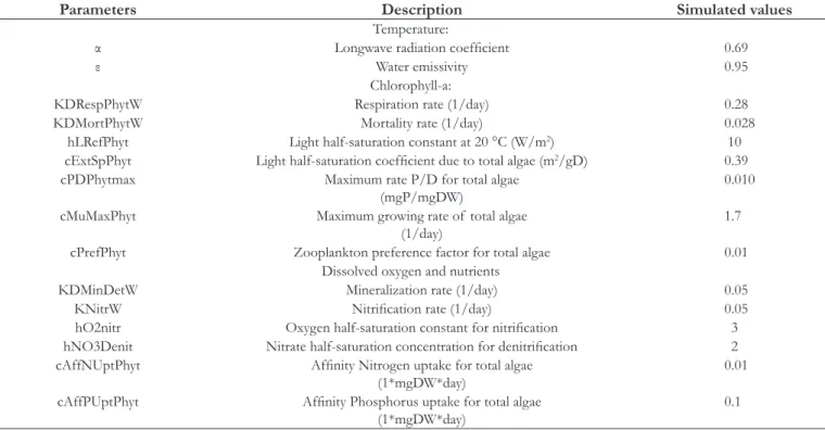
module was conducted by adjusting key parameters within the ranges reported in the literature. The parameters resulting from the calibration are summarized in Table 1.
Result analysis
After the calibration of water quality module, the metabolic
some cause-effect relationships between the reservoir metabolism and the limnological variables as well as the reservoir boundary conditions could be determined. Other relationships between these variables were determined through a linear regression. As a way to
evaluate model eficiency in representing the simulated variables, the square of the correlation coeficient R2 and Nash-Sutcliffe
eficiency NSE (NASH; SUTCLIFFE, 1970) were calculated.
RESULTS AND DISCUSSION
Water level modeling and inlow and loads
estimation
The simulation of the reservoir water levels through a water balance showed a good agreement with the measured values capturing the magnitudes and phases of water level changes during
the dry period (April-June). The Nash-Sutcliffe eficiency for this
simulation was 0.89 (Figure 4a). The increased water supply in the reservoir during the dry period led to a water level reduction of up to 3.0 m below reservoir weir height. Discrepancies between the simulation results and observation records were possibly due to several reasons: (a) the uncertainties inherent to the hydrological
model in estimating the reservoir inlows and loads from the
sub-basins; (b) the resolution of the reservoir bathymetry (biasing the relation depth versus volume); and (c) water release records as well as measured water level could be inaccurate.
As previously discussed, the adjustment of water level in the IPH-ECO lumped model started from the calibration of model cell resolution by varying its width (DX). For each DX
value, a relation depth versus volume was deined. By doing this, it was observed that as the slope of the line that deines model
depth versus volume relation approximates to the slope of the
Figure 4. IPH-II hydrological model calibration by adjusting the reservoir water levels through a water balance to the observed values during the simulation period (a); Depth versus Volume lines referred to the reservoir and the lumped model with a constant area (b); and the temporal variability of calculated water levels through the water balance of reservoir and by using the IPH-ECO lumped model (c). Table 1. Main parameters used in the calibration of IPH-ECO water quality module and their respective simulated values.
Parameters Description Simulated values
Temperature:
α Longwave radiation coeficient 0.69
ε Water emissivity 0.95
Chlorophyll-a:
KDRespPhytW Respiration rate (1/day) 0.28
KDMortPhytW Mortality rate (1/day) 0.028
hLRefPhyt Light half-saturation constant at 20 °C (W/m2) 10
cExtSpPhyt Light half-saturation coeficient due to total algae (m2/gD) 0.39
cPDPhytmax Maximum rate P/D for total algae (mgP/mgDW)
0.010
cMuMaxPhyt Maximum growing rate of total algae (1/day)
1.7
cPrefPhyt Zooplankton preference factor for total algae 0.01 Dissolved oxygen and nutrients
KDMinDetW Mineralization rate (1/day) 0.05
KNitrW Nitriication rate (1/day) 0.05
hO2nitr Oxygen half-saturation constant for nitriication 3 hNO3Denit Nitrate half-saturation concentration for denitriication 2 cAffNUptPhyt Afinity Nitrogen uptake for total algae
(1*mgDW*day)
0.01
cAffPUptPhyt Afinity Phosphorus uptake for total algae (1*mgDW*day)
line referred to the reservoir, the variation of lumped model results become similar to the variation of water balance results (Figures 4b and 4c). Hence, it is possible to consider a representative
cell width in the lumped model equivalent to the square root
of the line slope referred to the reservoir depth versus volume relation and obtain the same water level variation determined through the water balance (Figure 4c). The reservoir volume was
maintained by using the same linear coeficient of the line that describes reservoir depth versus volume relation in the equation
that describes the lumped model depth versus volume relation.
Inlow and nutrient yields from the 7 sub-basins were
applied together in the lumped model as they were coming from one single basin (Figure 5). The majority of external nutrient loadings occurred during the months of February, July and October following the heavy rainfall events. The increased nutrient loading could be associated with the application of fertilizers and pesticides in the period from July to October when soil in the basin is prepared for agriculture uses (VARGAS et al., 2013). Furthermore, a high nitrate concentration was observed in the SB-7 which may be
related to the waste-water treatment plant efluent and to the urban supericial drainage of Ana Rech district.
Water quality modeling
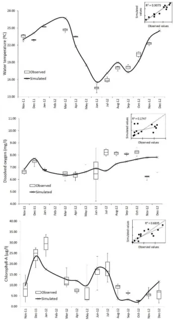
The IPH-ECO model was capable of reproducing the temporal variability of reservoir water temperature (Figure 6a) as shown by the good values of R2 and Nash-Sutcliffe eficiency NSE (Table 2). Reservoir water temperature was more inluenced by the variation of air temperature and solar radiation over the year.
Just like the water temperature, dissolved oxygen presented minor spatial changes, except in June as the box-plots referred to the observed values show (Figure 6b). In this month, the vertical mixing process occurred in the water column leading to an upward migration of nutrients and microorganisms in different points of the reservoir. If a 1D model was used to represent the mixing
and stratiication processes in the water column, then dissolved
oxygen would likely be different from the lumped model results. The temporal variability of dissolved oxygen concentration
during the simulation period was more inluenced by the luxes
of reaeration and phytoplankton production in the reservoir (Figures 7a and 7d). The DO concentration peak followed the phytoplankton production peak during December/2011. Likewise, in June an increase in DO concentration occurred continuing to grow over the next months, which may be related to the greater
intensity of reaeration luxes in these months.
Table 2. The square of the correlation coeficient (R2) and
Nash-Sutcliffe eficiency (NSE) to evaluate how good model
results agree with mean observed values of some limnological variables during the simulation period.
R2 NSE
Water temperature 0.91 0.90
Dissolved oxygen 0.17 0.12
Chlorophyll-a 0.68 0.67
Orthophosphate 0.48 0.39
Ammonium 0.52 0.42
Nitrate 0.89 0.87
Figure 5. IPH-II model results for total inlow and nutrient loads used as boundary conditions in the lumped model.
The low DO concentration during the last two months of
the simulation, as shown the ield data, may be associated with the
increased mineralization of detritus in the reservoir due to organic matter loading from the watershed which, by the way, was not described by the IPH-ECO model resulting in an overestimated DO concentration for this months.
The IPH-ECO model could capture phytoplankton biomass peaks in the months of December/2011 and June/2012 as shown in Figure 6c. The concentration peak in December/2011 was likely driven by the availability of light and nutrients. In this period,
the reservoir thermal stratiication occurs followed by increased
water temperature and light availability on the reservoir surface. Furthermore, an increased loading of nitrate and orthophosphate from watershed was observed in November and December/2011 (Figure 8c). The chlorophyll-a concentration peak in June may be associated with the sharp change in the reservoir water level
(Figure 4a) resulting in the vertical mixing and the upward movement of nutrients and microorganism from the bottom to the surface of the reservoir.
Simulated phytoplankton biomass would likely be higher if a 1D model able to represent water column processes was
applied, such as water mixing and the consequently increase in
nutrient concentrations and phytoplankton biomass in the reservoir
epilimnion. The chlorophyll-a peaks was also inluenced by the
increased reservoir residence time in the months of December (Figure 9) leading to a longer period of nutrient retention in the system and thus resulting in an increased chlorophyll-a concentration (Figure 6).
Another important aspect regarding the phytoplankton dynamics in the reservoir was zooplankton-grazing pressure. Over the simulation period, it was observed an inverse pattern between the simulated biomasses of zooplankton (Figure 10) Figure 7. Biogeochemical processes considered in the oxygen budget simulated by IPH-ECO model: reaeration (a); detritus mineralization
and phytoplankton. The lower grazing pressure at the beginning and at the end of the simulation period due to the reduction in zooplankton biomass may have enhanced the phytoplankton biomass in the reservoir.
Although phytoplankton biomass was simulated as a single functional group, some simulated parameters values obtained after the model calibration enabled some deductions about which functional groups have potentially dominated in the system. The majority of the biological parameters as hLRefPhyt, cExtSpPhyt, cMuMaxPhyt e cPrefPhyt, resulted within the value range reported in the literature for cyanobacteria (HAMILTON; SCHLADOW, 1997), indicating the dominance of this functional group over the reservoir during simulation period. Previous studies showed a high dominance of cyanobacterium- Anabaena Crassa in the Faxinal reservoir mostly during December and January when a phytoplankton biomass peak was observed followed by the diatom Asterionella formosa Hass (BECKER et al., 2009).
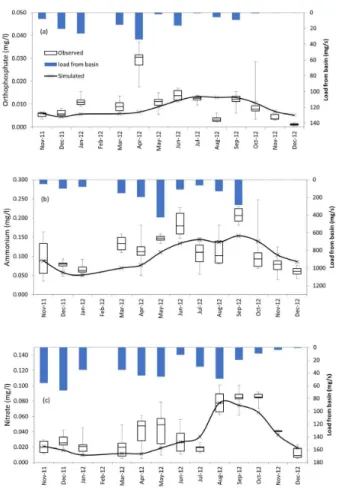
Simulated nutrient concentrations similarly followed the temporal pattern of the observed concentrations in the reservoir having a reasonable agreement with these values as shown by the statistical applied to this simulation (Table 2). However, the model was not able to reproduce some nutrient concentration peaks (Figure 8).
Some monitoring stations are located in shallower arms of the reservoir close to the sub-basin outlets where the concentration of nutrients is higher than in the other reservoir areas. Therefore, the lumped model better reproduced the nutrient dynamic in the center of reservoir and in the deeper areas nearer to the reservoir weir where a more homogeneous and dilute concentration of nutrients is observed. It was also noted that the high nutrient load from the basin that occurred in some months of the year was not able to cause an increase in the concentration of nutrients in the reservoir. However, the increased load of nitrate during November and December/2011 caused an increase in the phytoplankton biomass probably due to the higher uptake of nitrate by phytoplankton (Figure 6c). In the same way, the higher level of nitrate in August/2012 led to a considerable increase in this nutrient concentration in the reservoir.
Aquatic metabolism
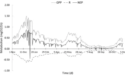
Model results indicated that the Faxinal reservoir is net autotrophic 97% of the simulation period being net heterotrophic on only some days in January, August and September (Figure 11). Temporal variability of gross primary production (GPP) followed the Figure 8. Adjustment of ortophosphate (a), amonium (b) and
nitrate (c) simulated values to the box-plots of the observed values at the monitoring stations in the Faxinal Reservoir including the nutrient loads from the sub-basins.
Figure 9. Simulated monthly mean residence time of the Faxinal reservoir and simulated phytoplankton biomass.
production of phytoplankton biomass in the reservoir (Figure 7d). Furthermore, the variation of respiration rate followed the temporal
variability of the luxes of mineralization and phytoplankyon
respiration in the reservoir (Figures 7b and 7e). Net ecosystem production (NEP) was negative (R>GPP) presenting a value of -0.45 mgO2 / l / s on a single day in January when it was observed a peak in the mineralization and in the phytoplankton respiration (Figures 7b and 7f).
On some days in August and September the reservoir was net heterotrophic. This behavior may have been associated with
the intensiication of nitriication process (Figure 7c) as well as the reduction of phytoplankton production in this period (Figure 7d). Good correlations were obtained between the metabolic
rates (GPP and R) and the simulated water quality variables as
well as the external loading of nutrients as shown by the values of the regression line R2.
Both GPP and R were positively correlated with the concentration of detritus (Figure 12). The model results showed a low concentration of detritus in the reservoir since only autochthonous contribution was considered in the simulation, not taking into account the external loading of organic matter, which may have
a signiicant effect on the production of detritus in the reservoir.
Therefore, the increased concentration of autochthonous detritus
was more related to the phytoplankton mortality lux, which was
directly related to the phytoplankton biomass and the gross primary production in the reservoir. Respiration rate also increased with
the rise in detritus concentration since the mineralization lux,
which is directly related to respiration, is positively correlated with the organic matter concentration.
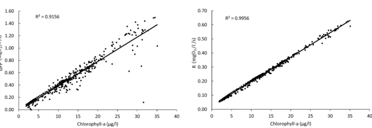
Another variable that had a strong positive correlation with GPP and R was chlorophyll-a biomass (Figure 13). A weak correlation between metabolism and chlorophyll-a was found for concentrations higher than 20 µg/L suggesting that other factors may have affected the time variation of GPP in cases like this. Chlorophyll-a biomass at levels higher than 20 µg/L was observed in the reservoir arms near the sub-basin outlets where an increased loading of detritus from uplands was also observed. Therefore, allochthonous organic matter from uplands may also
have inluenced the gross primary production in the reservoir.
The strong correlation between chlorophyll-a and R indicated that the effect of phytoplankton respiration on R is higher than the effect of detritus mineralization.
External loadings of nitrate, ammonium and inlows from the basin were not signiicantly correlated with metabolic rates
whereas a good correlation was found with orthophosphate loading during rainfall periods (Figure 14). Phosphorus loading from the basin had an indirect effect on the increased rates of GPP and R
since irst led to an increase in phytoplankton biomass, which in
turn had a direct relationship with gross primary production and respiration in the reservoir.
CONCLUSION
Model results indicated that the prevailing net autotrophic metabolism of the Faxinal reservoir is mainly driven by phytoplankton biomass. During the simulation period a long dry period started, leading to a reduction in the reservoir water level and at the same time to an increase in water residence time. Additionally the availability of light and autochthonous nutrients contributed to the increased phytoplankton biomass in the reservoir.
Following the temporal pattern of the Faxinal reservoir, metabolism of other deep subtropical reservoirs where the
stratiication of water column persists for a long period during
the year and the ratio of the areas of the basin and reservoir is small tend to respond more to the internal dynamics of the
system than the loadings and inlows from the basin. However,
at a local scale it is important to know the possible effects of the land use changes in the basin (which has no soil use planning) on the metabolism of the Faxinal reservoir. Moreover, as a man-made
aquatic system the Faxinal reservoir is subject to temporal and
spatial changes related to its water withdrawal operation over the year that in turn alter its water residence time and hydrodynamics. In this way, the temporal and spatial pattern of the limnological variables considered in this work tend to become less uniform over the time following a pattern different from that simulated in the lumped model for the study period.
A spatial analysis of metabolism besides the temporal analysis developed in this work may reveal different patterns enabling a better comprehension of the biogeochemical processes at different scales in the reservoir. Therefore, a distributed spatial
approach able to represent hydrodynamics and water quality of
the reservoir coupled with hydrological variables of the basin is strongly recommended in future works.
Figure 13. Linear regression applied between metabolic rates of GPP and R and simulated chlorophyll-a biomass in the reservoir.
REFERENCES
ANTENUCCI, J. P.; TAN, K. M.; EIKAAS, H. S.; IMBERGER, J. The importance of transport processes and spatial gradients on in situ estimates of lake metabolism. Hydrobiologia, v. 700, n. 1, p. 9-21, 2012. http://dx.doi.org/10.1007/s10750-012-1212-z.
BARROS, N.; COLE, J. J.; TRANVIK, L. J.; PRAIRIE, Y. T.; BASTVIKEN, D.; HUSZAR, V. L. M.; GIORGIO, P.; ROLAND, F. Carbon emission from hydroelectric reservoirs linked to reservoir age and latitude. Nature Geoscience, v. 4, n. 9, p. 593-596, 2011.
BECKER, V.; HUSZAR, V. L. M.; CROSSETTI, L. O. Responses of phytoplankton functional groups to the mixing regime in a deep subtropical reservoir. Hydrobiologia, v. 628, n. 1, p. 137-151, 2009. http://dx.doi.org/10.1007/s10750-009-9751-7.
BECKER, V.; HUSZAR, V. L. M.; FLORES, L. N.; PADISÁK, J.
Phytoplankton equilibrium phases during thermal stratification in
a deep subtropical reservoir. Freshwater Biology, v. 53, n. 5, p. 952-963, 2008. http://dx.doi.org/10.1111/j.1365-2427.2008.01957.x.
BRAVO, J. M.; PICCILLI, D. G. A.; COLLISCHONN, W.; TASSI, R.; MELLER, A.; TUCCI, C. E. M. Avaliação visual e numérica da
calibração do modelo hidrológico IPH-II com fins educacionais.
In: SIMPÓSIO BRASILEIRO DE RECURSOS HÍDRICOS, 17., 2007. Anais...
CARMOUZE, J. P. O metabolismo dos ecossistemas aquáticos:
fundamentos teóricos, métodos de estudo e análises químicas. São Paulo: FAPESP, 1994.
CASULLI, V. Semi-implicit finite difference methods for the
two-dimensional shallow water equations. Journal of Computational Physics, v. 86, n. 1, p. 56-74, 1990. http://dx.doi.org/10.1016/0021-9991(90)90091-E.
CAVALCANTI, J. R. A. Inluência da hidrodinâmica no metabolismo de lagos rasos. 2013. 92 f. Dissertação (Mestrado em Recursos Hídricos e Saneamento Ambiental) – Universidade Federal do Rio Grande do Sul, Porto Alegre, 2013.
CHENG, R. T.; CASULLI, V.; GARTNER, J. W. Tidal, residual, intertidal mudflat model and its applications to San Francisco Bay, California. Estuarine, Coastal and Shelf Science, v. 36, n. 3, p. 235-280, 1993. http://dx.doi.org/10.1006/ecss.1993.1016.
COLE, J. J.; PACE, M. L.; CARPENTER, S. R.; KITCHELL, J. F. Persistence of net heterotrophy in lakes during nutrient addition and food web manipulations. Limnology and Oceanography, v. 45, n. 8, p. 1718-1730, 2000. http://dx.doi.org/10.4319/lo.2000.45.8.1718.
COLOSO, J. J.; COLE, J. J.; PACE, M. L. Difficulty in discerning
drivers of lakes ecosystem metabolism with high-frequency data.
Ecosystems, v. 14, n. 6, p. 935-948, 2011. http://dx.doi.org/10.1007/ s10021-011-9455-5.
EVANS, M. A.; MACINTYRE, S.; KLING, G. W. Internal wave effects on photosynthesis: experiments, theory, and modeling. Limnology and Oceanography, v. 53, n. 1, p. 339-353, 2008. http:// dx.doi.org/10.4319/lo.2008.53.1.0339.
FRAGOSO JÚNIOR, C. R.; FERREIRA, T. F.; MARQUES, D. M. Modelagem ecológica em ecossistemas aquáticos. São Paulo: Oficina de Textos, 2009.
FRAGOSO JÚNIOR, C. R.; MARQUES, D. M.; COLLISCHONN, W.; VAN NES, E. H. Modelagem ecológica como ferramenta
auxiliar para restauração de Lagos Rasos Tropicais e Subtropicais.
Revista Brasileira de Recursos Hídricos, v. 15, n. 2, p. 15-25, 2010. http://dx.doi.org/10.21168/rbrh.v15n2.p15-25.
GAL, G.; PARPAROV, A.; WAGNER, U.; ROZENBERG, T. Testing the impact of management scenarios on water quality using an ecosystem model. Israel: Israel Oceanographic and Limnological Research, Kinneret Limnological Laboratory, , 2002.
GERMANO, A.; TUCCI, C. E. M.; SILVEIRA, A. L. L. Estimativa dos parâmetros do modelo IPH II para algumas bacias urbanas brasileiras. Revista Brasileira de Recursos Hídricos, v. 3, n. 4, p. 103-120, 1998. http://dx.doi.org/10.21168/rbrh.v3n4.p103-120.
HAMILTON, D. P.; SCHLADOW, S. G. Prediction of water
quality in lakes and reservoirs. Part I – Model description. Ecological Modelling, v. 96, n. 1-3, p. 91-110, 1997. http://dx.doi.org/10.1016/ S0304-3800(96)00062-2.
HANSON, P. C.; BADE, D. L.; CARPENTER, S. R.; KRATZ, T. K. Lake metabolism: Relationships with dissolved organic carbon and phosphorus. Limnology and Oceanography, v. 8, n. 3, p. 1112-1119, 2003. http://dx.doi.org/10.4319/lo.2003.48.3.1112.
HANSON, P. C.; CARPENTER, S. R.; ARMSTRONG, D. E.; STANLEY, E. H.; KRATZ, T. K. Lake dissolved inorganic carbon and dissolved oxygen: Changing drivers from days to decades. Ecological Monographs, v. 76, n. 3, p. 343-363, 2006. http://dx.doi. org/10.1890/0012-9615(2006)076[0343:LDICAD]2.0.CO;2.
HODGES, B. R.; IMBERGER, J.; SAGGIO, A.; WINTERS, K. B. Modeling basin-scale internal waves in a stratified lake. Limnology and Oceanography, v. 45, n. 7, p. 1603-1620, 2000. http://dx.doi. org/10.4319/lo.2000.45.7.1603.
KIM, Y.; ROULET, N. T.; LI, C.; FROLKING, S.; STRACHAN, I. B.; PENG, C.; TEODORU, C. R.; PRAIRIE, Y. T.; TREMBLAY, A. Simulating the CO2 exchange in boreal ecosystems flooded by reservoirs. Ecological Modelling, v. 327, p. 1-17, 2012. http://dx.doi. org/10.1016/j.ecolmodel.2016.01.006.
KÖPPEN, W. Das geographische System der Klimate-Handbuch der Klimatologie: part C. Berlin: Gerbrüder Bornträger, 1936. v. 1.
Global Biogeochemical Cycles, v. 24, n. 2, p. 1-7, 2010. http://dx.doi. org/10.1029/2009GB003618.
MAROTTA, H.; DUARTE, C. M.; PINHO, L.; ENRICH-PRAST, A. Rainfall leads to increased pCO2 in Brazilian coastal lakes. Biogeosciences, v. 7, n. 5, p. 1607-1614, 2010. http://dx.doi. org/10.5194/bg-7-1607-2010.
NASH, J. E.; SUTCLIFFE, J. V. River flow forecasting through conceptual models, Part I: a discussion of principles. Journal of Hydrology, v. 10, n. 3, p. 282-290, 1970. http://dx.doi.org/10.1016/0022-1694(70)90255-6.
ODUM, H. T. Primary production in flowing waters. Limnology and Oceanography, v. 1, n. 2, p. 102-117, 1956. http://dx.doi. org/10.4319/lo.1956.1.2.0102.
PANNARD, A.; BEISNER, B. E.; BIRD, D. F.; BRAUN, J.; PLANAS, D.; BORMANS, M. Recurrent internal waves in a
small lake: Potential ecological consequences for metalimnetic
phytoplankton populations. Limnology and Oceanography: Fluids and Environments, v. 1, p. 91-109, 2011.
RAYMOND, P. A.; HARTMANN, J.; LAUERWALD, R.; SOBEK, S.; MCDONALD, C.; HOOVER, M.; BUTMAN, D.; STRIEGL, R.; MAYORGA, E.; HUMBORG, C.; KORTELAINEN, P.; DÜRR, H.; MEYBECK, M.; CIAIS, P.; GUTH, P. Global carbon dioxide emissions from inland waters. Nature, v. 503, n. 7476, p. 355-359, 2013. PMid:24256802. http://dx.doi.org/10.1038/nature12760.
SOBEK, S.; SÖDERBÄCK, B.; KARLSSON, S.; ANDERSSON, E.; BRUNBERG, A. K. A carbon budget of a small humic lake: An example of the importance of lakes for organic matter cycling in boreal catchments. Ambio, v. 35, n. 8, p. 469-475, 2006. PMid:17334054. http://dx.doi.org/10.1579/0044-7447(2006)35[469:ACBOAS] 2.0.CO;2.
SOLOMON, C. T.; BRUESEWITZ, D. A.; RICHARDSON, D. C.; ROSE, K. C.; VAN DE BOGERT, M. C.; HANSON, P. C.; KRATZ, T. K.; LARGET, B.; ADRIAN, R.; BABIN, L. B.; CHIU, C.; HAMILTON, D. P.; GAISER, E. E.; HENDRICKS, S.; ISTVÀNOVICS, V.; LAAS, A.; O’DONNELL, D. M.; PACE, M. L.; RYDER, E.; STAEHR, P. A.; TORGERSEN, T.; VANNI, M. J.; WEATHERS, K. C.; ZHU, G. Ecosystem respration: Drivers of daily variability and background respiration in lakes around the globe. Limnology and Oceanography, v. 58, n. 3, p. 849-866, 2013. http://dx.doi.org/10.4319/lo.2013.58.3.0849.
SOUZA, R. S. Regulação espaço-temporal e implicações das mudanças climáticas na emissão de gases do efeito estufa em ecossistemas aquáticos subtropicais. 2013. 190 f. Tese (Doutorado em Recursos Hídricos e Saneamento Ambiental) – IPH, Universidade Federal do Rio Grande do Sul, Porto Alegre, 2013.
STAEHR, P. A.; JENSEN, K. S.; RAUN, A. L.; NILSSON, B.; KIDMOSEC, J. Drivers of metabolism and net heterotrophy in contrasting lakes. Limnology and Oceanography, v. 55, n. 2, p. 817-830, 2010. http://dx.doi.org/10.4319/lo.2009.55.2.0817.
TESTA, J. M.; LI, Y.; LEE, Y. J.; LI, M.; BRADY, D. C.; DI TORO, D. M.; KEMP, W. M.; FITZPATRICK, J. J. Quantifying the effects of nutrient loading on dissolved O2 cycling and hypoxia in Chesapeake Bay using a coupled hydrodynamic-biogeochemical model. Journal of Marine Systems, v. 139, p. 139-158, 2014. http:// dx.doi.org/10.1016/j.jmarsys.2014.05.018.
VAN DE BOGERT, M. C.; CARPENTER, S. R.; COLE, J. J.; PACE, M. L. Assessing pelagic and benthic metabolism using free water measurements. Limnology and Oceanography, Methods, v. 5, n. 5, p. 145-155, 2007. http://dx.doi.org/10.4319/lom.2007.5.145.
VARGAS, T.; ADAMI, M. V. D.; AVER, E. A. S.; BELLADONA, R.; ZAGO, M. A.; FRIZZO, E. E. Monitoramento hidroquímico dos córregos afluentes da represa faxinal, Caxias do Sul – RS. In: SIMPÓSIO BRASILEIRO DE RECURSOS HÍDRICOS,
20., 2013, Bento Gonçalves. Anais... Porto Alegre: ABRH, 2013.
ZHANG, H.; HUANG, G. H.; WANG, D.; ZHANG, X.; LI, G.; AN, C.; CUI, Z.; LIAO, R.; NIE, X. An integrated multi-level watershed-reservoir modeling system for examining hydrological and biogeochemical processes in small prairie watersheds. Water Research, v. 46, n. 4, p. 1207-1224, 2012. PMid:22212883. http:// dx.doi.org/10.1016/j.watres.2011.12.021.
Authors contributions
Vinicius Teixeira Tambara: Literature survey; data processing application in the model; model calibration; analysis and discussion of results and article wrote.
Carlos Ruberto Fragoso Júnior: Study joint supervision; result discussion and text revision.