www.geosci-model-dev.net/8/1547/2015/ doi:10.5194/gmd-8-1547-2015
© Author(s) 2015. CC Attribution 3.0 License.
NEMO–ICB (v1.0): interactive icebergs in the NEMO ocean model
globally configured at eddy-permitting resolution
R. Marsh1, V. O. Ivchenko1, N. Skliris1, S. Alderson2, G. R. Bigg3, G. Madec2,4, A. T. Blaker2, Y. Aksenov2, B. Sinha2, A. C. Coward2, J. Le Sommer5, N. Merino5, and V. B. Zalesny6
1University of Southampton, National Oceanography Centre, Southampton, UK
2National Oceanography Centre, Southampton, European Way, Southampton SO14 3ZH, UK 3Department of Geography, University of Sheffield, Sheffield, UK
4LOCEAN-IPSL, CNRS-IRD-UPMC-MNHN, Paris, France 5LGGE, UMR5183, CNRS-UJF, Grenoble, France
6Institute of Numerical Mathematics, Russian Academy of Sciences, Gubkin St. 8, Moscow, 119333, Russia
Correspondence to:R. Marsh ([email protected])
Received: 23 June 2014 – Published in Geosci. Model Dev. Discuss.: 25 August 2014 Revised: 27 February 2015 – Accepted: 13 April 2015 – Published: 27 May 2015
Abstract. An established iceberg module, ICB, is used in-teractively with the Nucleus for European Modelling of the Ocean (NEMO) ocean model in a new implementation, NEMO–ICB (v1.0). A 30-year hindcast (1976–2005) sim-ulation with an eddy-permitting (0.25◦) global configuration
of NEMO–ICB is undertaken to evaluate the influence of ice-bergs on sea ice, hydrography, mixed layer depths (MLDs), and ocean currents, through comparison with a control sim-ulation in which the equivalent iceberg mass flux is applied as coastal runoff, a common forcing in ocean models. In the Southern Hemisphere (SH), drift and melting of icebergs are in balance after around 5 years, whereas the equilibration timescale for the Northern Hemisphere (NH) is 15–20 years. Iceberg drift patterns, and Southern Ocean iceberg mass, compare favourably with available observations. Freshwater forcing due to iceberg melting is most pronounced very lo-cally, in the coastal zone around much of Antarctica, where it often exceeds in magnitude and opposes the negative fresh-water fluxes associated with sea ice freezing. However, at most locations in the polar Southern Ocean, the annual-mean freshwater flux due to icebergs, if present, is typically an order of magnitude smaller than the contribution of sea ice melting and precipitation. A notable exception is the south-west Atlantic sector of the Southern Ocean, where iceberg melting reaches around 50 % of net precipitation over a large area. Including icebergs in place of coastal runoff, sea ice concentration and thickness are notably decreased at most
locations around Antarctica, by up to∼20 % in the eastern
Weddell Sea, with more limited increases, of up to∼10 %
in the Bellingshausen Sea. Antarctic sea ice mass decreases by 2.9 %, overall. As a consequence of changes in net fresh-water forcing and sea ice, salinity and temperature distribu-tions are also substantially altered. Surface salinity increases by∼0.1 psu around much of Antarctica, due to suppressed coastal runoff, with extensive freshening at depth, extend-ing to the greatest depths in the polar Southern Ocean where discernible effects on both salinity and temperature reach 2500 m in the Weddell Sea by the last pentad of the simu-lation. Substantial physical and dynamical responses to ice-bergs, throughout the global ocean, are explained by rapid propagation of density anomalies from high-to-low latitudes. Complementary to the baseline model used here, three pro-totype modifications to NEMO–ICB are also introduced and discussed.
1 Introduction
influence on the open ocean (Bigg and Wadley, 1996; Bigg et al., 1997).
In order to accommodate the climatic influence of ice-bergs, principally through the freshwater input to the ocean, it is necessary to model their statistical distribution, rather than track large numbers of individual bergs (Hunke and Comeau, 2011). Interactive ocean–iceberg modelling began with the development of an ocean-forced iceberg trajectory model (Bigg and Wadley, 1996). An iceberg momentum bal-ance accounts for Coriolis and pressure gradient forces, plus drag forces from ocean, wind, waves, and sea ice. Along each trajectory, iceberg mass is reduced according to parameteri-zations of basal melting, buoyant convection, and wave ero-sion. This model has been extensively used and validated in the Arctic (e.g. Bigg and Wadley, 1996) and Antarctic (Glad-stone et al., 2001), as well as for palaeoclimate studies (e.g. Watkins et al., 2007).
The iceberg model was subsequently coupled with the Fine-Resolution Greenland Sea and Labrador Sea (FRU-GAL) ocean model, which features a curvilinear grid system with a North Pole centred in Greenland, ensuring reasonably high resolution (20–50 km) in the northern Atlantic and Arc-tic (Wadley and Bigg, 2000). This coupling allows for feed-back between iceberg meltwater and the surface ocean dy-namics and thermodydy-namics (Levine and Bigg, 2008). For a given calving flux, a distribution of icebergs is specified in terms of size, with characteristic length, width and thickness. In separate developments, modified versions of the Bigg and Wadley (1996) and Bigg et al. (1997) iceberg model have been coupled with the ECBilt-CLIO Earth System Model (Jongma et al., 2009) and with CM2G, a next-generation GFDL (Geophysical Fluid Dynamics Laboratory) climate model, featuring an isopycnal-coordinate ocean component (Martin and Adcroft, 2010; henceforth MA10). Jongma et al. (2009) found that freshening and cooling influences of icebergs enhance sea ice area by 12 and 6 %, respectively. MA10 conversely found that sea ice cover is generally thin-ner and less compact with icebergs, compared to a control experiment in which fresh water enters the ocean at the coast and stimulates sea ice growth. They found the strongest de-creases in sea ice concentration of 6–8 % in the Amundsen, Bellingshausen, Weddell, and D’Urville seas, i.e. along the major export routes for icebergs. The reduced freshwater in-put over continental shelf regions in experiments with ice-bergs (in particular, the flux of “bergy bits”) enhances deep-water formation in CM2G, leading to an increase of up to 10 % in the production rate of model Antarctic Bottom Wa-ter.
It should be noted that the iceberg mass fluxes and dis-tributions in CM2G – and the aforementioned impacts – are associated with calving rates, in balance with precipitation over ice sheets, that are rather different from observations. We also note that Jongma et al. (2009) distributed Antarctic runoff globally in the control experiment, in contrast to the control run with CM2G, which could explain the opposing
sea ice trends associated with the introduction of icebergs to ECBilt-CLIO and CM2G.
In the present study, a modified version of the Bigg and Wadley (1996) and Bigg et al. (1997) iceberg model, devel-oped by MA10, is coupled to an eddy-permitting global im-plementation of the Nucleus for European Modelling of the Ocean (NEMO) (Madec, 2008), to simulate the trajectories and melting of calved icebergs – from Antarctica, Greenland, and small northern ice caps – in the presence of mesoscale variability and fine-scale dynamical structure. In contrast, both MA10 and Jongma et al. (2009) included icebergs in models with coarse (non-eddy resolving) ocean resolution.
The rest of the paper is organized as follows. In a model description section (Sect. 2), we provide details of the ice-berg module (ICB), NEMO configuration, NEMO–ICB im-plementation, specified calving, experimental design, and di-agnostics. In a model validation section (Sect. 3), we con-sider first the distribution of icebergs and the associated freshwater flux, followed by differences, attributed to the inclusion of icebergs, in sea ice, hydrography, mixed layer depths (MLDs) and ocean currents. In an additional section (Sect. 4), we describe prototype modifications of NEMO– ICB, in relation to the baseline configuration used here. In a summary and discussion section (Sect. 5), we compare and contrast our present results with observations and pre-vious simulations, before highlighting some caveats related to physical processes that are yet to be included in cou-pled iceberg–ocean models. We conclude with details of code availability.
2 Model description 2.1 The iceberg module
The ICB (for ICeBergs) module is based on the original model of Bigg et al. (1997), as recently adapted for cou-pling to the CM2G climate model by MA10. Collections of icebergs are treated as Lagrangian particles, with the distri-bution of icebergs by size derived from observations. With increasing size (e.g. thickness ranging from 40 to 250 m), smaller collections of icebergs are represented per particle – see Bigg et al. (1997) and MA10 for full details. The mo-mentum balance for icebergs comprises the Coriolis force, air and water form drags, the horizontal pressure gradient force, a wave radiation force, and interaction with sea ice. The mass balance for an individual iceberg is governed by basal melting, buoyant convection at the sidewalls, and wave erosion (see Bigg et al., 1997). All respective equations are the same as detailed in MA10, so are not repeated here.
of our biggest represented icebergs is∼1 km, and such ice-bergs are generally well dispersed around Antarctica, Green-land, and Arctic ice caps. Only near release sites will there be a sufficient iceberg density to perhaps impact sea ice mo-tion, which is determined on model grid scales that are more than 10 times larger than our largest icebergs. Independent of iceberg concentration, the impact of sea ice drag on ice-bergs is observed to be minimal around 80–90 % of the time (Lighey and Hellmer, 2001), so the momentum interaction term, and any resulting feedback, may be regarded as second order. Only when the pack is concentrated does this change, and then there is a switch to the berg being carried by the sea ice. This step change in iceberg dynamics is not yet param-eterized. We also assume that icebergs are oriented at 45◦ relative to the wind, with the wind to the left (right) in the Northern Hemisphere (NH) (Southern Hemisphere – SH), as outlined in Bigg et al. (1997). This may or may not be the case in reality. Thus, any stress provided from the sea ice model grid is likely to be only approximate. For these rea-sons, a simple drag law – as implicit here (Eq. A.2c in MA10) – is realistic for iceberg interaction with sea ice. For higher-resolution ocean models, with grid-cell dimensions of just a few kilometres, it would be necessary to more explicitly ac-count for momentum transfers between icebergs and sea ice, but the present resolution prohibits such representation.
Sea ice concentration and thickness can also be impacted by freshwater fluxes from melting. Given the scale issues mentioned above, but the spreading of meltwater widely across the surface, one can argue that the effect of meltwater on these sea ice parameters is likely to be much greater than the imprecisely represented and resolved dynamical effect.
2.2 NEMO version and configuration
Interactive icebergs are implemented in NEMO v3.5, in a model option known as NEMO–ICB. The source code and forcing files used in the configurations presented here are available to registered NEMO users (see “Code avail-ability”). The NEMO ocean model component is cou-pled to either the Louvain-la-Neuve sea ice model (LIM2) with viscous-plastic rheology, formulated by Fichefet and Maqueda (1997), or the Los Alamos National Laboratory sea ice model version 4.1 (CICE v4.1; see Hunke and Lip-scomb, 2010). After initial NEMO–ICB development with LIM2 (Marsh et al., 2014), the results presented here are ob-tained with NEMO coupled to CICE. While testing of the latest NEMO versions is ongoing, validation of v3.4 demon-strated substantial improvements in surface physics over v3.2 (Megann et al., 2014).
2.3 NEMO–ICB implementation – baseline and prototype versions
Implementation of the ICB module within the NEMO frame-work differs from implementation of icebergs in the sea ice
module of CM2G (MA10). The NEMO–ICB implementa-tion was motivated by anticipated model development. Ice-bergs in the real world – up to 250 m thick in the model – are largely submerged into the ocean, and therefore influ-enced by vertical temperature gradients and current shears. For physically correct model representation of iceberg–ocean interaction, model icebergs should correspondingly be sub-merged in the model ocean – difficult to code within the CM2G scheme.
The results presented here are obtained for icebergs in-teracting with surface currents and surface temperatures – henceforth denoted the baseline version (for the available code, see “Code availability”). Besides the baseline version of the code, a number of optional modifications have been implemented and are currently being tested. In particular, this includes an option for advection of icebergs with depth-averaged currents, extending the dynamics routines to 3-D settings with minor code changes. Other optional modifica-tions to the baseline version of the code include iceberg in-teraction with shallow bathymetry and computation of melt-ing rates with the 3-D temperature field. These modifications are further described and discussed in Sect. 4 but are not yet readily available in the code.
As icebergs melt, freshwater is added to the surface level of the ocean model with salinity 0 psu – effectively a frozen fraction of the total runoff in NEMO, re-distributed – fresh-ening the ocean surface layer. There is no associated heat flux in the experiment presented here, although the option exists in NEMO–ICB for meltwater with a nominal temperature of
−4◦C to mix with the ocean. The additional mass flux
asso-ciated with iceberg melt also alters the free surface height in NEMO.
2.4 Iceberg calving
Climatological iceberg calving rates are distributed realisti-cally around coastlines in high latitudes of the NH and SH (as shown in Fig. 2a of Levine and Bigg, 2008), and the im-plied calving events are constant through time. The initial length/width ratio for all newly calved icebergs is 1.5, and size distributions are specified as in MA10.
The total calving rate specified for Antarctica is 1140 Gt year−1, compared to 1332 Gt year−1in Gladstone et al. (2001) and 1375 Gt year−1in Levine and Bigg (2008) – from 1500 km3year−1in the latter study, taking a standard density for ice, at 0◦C, of 916.7 kg m−3. While giant ice-bergs are unrepresented here, their absence does not account for these differences. Our Antarctic calving rate comprises 51.6 % of total freshwater flux into the Southern Ocean from Antarctica (2210 Gt year−1), prescribed as 100 % runoff in the absence of icebergs.
ice sheet, with minor contributions from Axel Heiberg Is-land, Ellesmere IsIs-land, Devon IsIs-land, Bylot IsIs-land, Baffin Island, Svalbard, Franz Josef Island, Novaya Zemlya, and Severnaya Zemlya. Around Greenland, the calving rate com-prises around 50 % of total freshwater flux into the North Atlantic from the ice sheet.
It is noteworthy that our calving rates are derived from a mass balance calculation of around 2000, before melt and discharge from ice sheets began to increase significantly. Rignot et al. (2011) report steadily increasing rates of ice sheet mass discharge (remote sensing of ice motion and thickness) over 1992–2009, ∼500 to ∼630 Gt year−1 for
Greenland, and∼2140 to ∼2300 Gt year−1 for Antarctica.
The partitioning of this discharge between calving and melt-ing (basal meltmelt-ing of outlet glaciers and ice shelves) is poorly known and undoubtedly changing rapidly, but it is likely that recent calving rates are substantially higher than those used to develop earlier climatological rates, and trending upwards. In summary, our calving rates are conservative in the con-text of these ongoing changes, akin to “pre-industrial” esti-mates. The oceanographic and sea ice impacts reported here are therefore also likely to be conservative.
2.5 Experimental design
In common with preceding NEMO development (e.g. Megann et al., 2014), we undertook 30-year hindcast ex-periments, here for the period 1976–2005, with the 0.25◦ resolution (eddy-permitting) global configuration known as ORCA025. We henceforth refer to corresponding NEMO ex-periments (without icebergs) as CONTROL, and NEMO– ICB experiments (with icebergs) as ICEBERG. In CON-TROL, liquid freshwater (runoff) fluxes are prescribed at coastal grid cells around Antarctica, Greenland, and the smaller icecaps. This reference run is designed to empha-size the importance of icebergs in transporting freshwater, and we stress here that most DRAKKAR (see Megann et al., 2014) simulations with ORCA025 now use “static” 2-D maps of freshwater flux due to icebergs – e.g. for the South-ern Ocean, the map is derived from Silva et al. (2006), or freshwater from melting icebergs is homogeneously spread south of 60◦S.
In ICEBERG, runoff around ice sheets is re-partitioned be-tween iceberg calving and reduced runoff at coastal grid cells (spatially distributed as in CONTROL), such that the global ocean receives exactly the same freshwater flux in CON-TROL and ICEBERG. Seasonal cycles of runoff are pre-served through small adjustments at selected locations, while iceberg calving is constant throughout the year. We cannot guarantee that global-mean salinity will remain the same in both experiments, due to partial dependence of evaporation on sea surface temperature (SST), and the salinity relaxation scheme of NEMO. However, these effects on global-mean salinity are found to be very small (see Sect. 3.3).
2.6 Diagnostics
For a given time interval, the locations and properties of indi-vidual iceberg particles (each representative of varying num-bers of icebergs in a given size class) are saved in a set of files that may be post-processed to obtain selected distribu-tions and tracks for individual icebergs.
Integral diagnostics are written to the tracer files of stan-dard NEMO output. Table 1 lists the full suite of these diag-nostics, along with corresponding variable names and units. Most iceberg diagnostics are 2-D fields on the NEMO ocean model mesh. Particularly useful instantaneous measures of the iceberg model include the virtual coverage by icebergs – virtual in the sense that total grid-cell area is the sum of open water and sea ice, consistent with the very small frac-tional area for icebergs in the size categories considered here. Other important diagnostics are the melt rate of icebergs, in total and partitioned into three components named in the tracer files as “buoyancy component of iceberg melt rate” (basal melting); “convective component . . . ” (sidewall melt-ing); “erosion component . . . ” (wave erosion).
3 Model evaluation
We first consider the spin-up of NEMO–ICB in terms of total iceberg volume. We then illustrate typical near-equilibrium iceberg distributions, based on year 26–30 (hindcast years 2001–2005) averages. We subsequently examine sea ice con-centration and thickness, hydrography, MLDs, and prelimi-nary evidence for iceberg influences on the global ocean cir-culation.
3.1 Iceberg distribution and freshwater flux
Table 1.Iceberg diagnostics saved in the standard NEMO tracer files.
Diagnostic Variable name Units
Calving mass input calving kg s−1
Calving heat flux calving_heat –
Melt rate of icebergs+bits berg_floating_melt kg m−2s−1 Accumulated ice mass by class berg_stored_ice kg
Melt rate of icebergs berg_melt kg m−2s−1 Buoyancy component of iceberg melting berg_buoy_melt kg m−2s−1 Erosion component of iceberg melting berg_eros_melt kg m−2s−1 Convective component of iceberg melting berg_conv_melt kg m−2s−1 Virtual coverage by icebergs berg_virtual_area m2 Mass source of bergy bits bits_src kg m−2s−1 Melt rate of bergy bits bits_melt kg m−2s−1 Bergy bit density field bits_mass kg m−2
Iceberg density field berg_mass kg m−2
Calving into iceberg class berg_real_calving kg s−1
5 10 15 20 25 30
0 500 1000 1500
ICEBERG MASS (Gt)
Years
NH SH
SH North of 66oS Total
Figure 1. Time series of total iceberg mass (1 Gt=109 tonne
=1012kg); southern hemispheric and northern hemispheric iceberg mass is indicated by the red and blue lines, respectively. Southern hemispheric iceberg mass north of 66◦S (dashed red line) is shown for comparison with observations of Tournadre et al. (2012).
of iceberg mass between the hemispheres is therefore likely to be greater than in the model.
The year 26–30 mean global iceberg mass of 800–1000 Gt is considerably lower than the∼6000 Gt obtained after
100-year spin-up of CM2G (MA10). However, as further dis-cussed below, the high global iceberg mass in CM2G is as-sociated with excessive calving rates in the Pacific sector of Antarctica (see Fig. 9a in MA10). For southern hemispheric regions where observations are available, total iceberg mass in NEMO–ICB appears to be realistic: ∼200 Gt north of 66◦S in the Southern Ocean (dashed red line in Fig. 1) com-pares favourably with estimates based on satellite observa-tions over 2002–2010 (Tournadre et al., 2012, their Figs. 5 and 6).
Global iceberg mass budgets for NEMO–ICB and CM2G are summarized in Table 2. Both models are close to a bal-ance between calving and melting, with the imbalbal-ances (net
melting) just under 5 Gt year−1for both simulations, corre-sponding to 0.37 and 0.19 % of the total calving rates in NEMO–ICB and CM2G, respectively. In spite of adopting the same parameterizations as MA10, we obtain somewhat different global rates and partitioning (see Table 2). As in CM2G, wave erosion flux is dominant in NEMO–ICB, but basal melt flux is less substantial (17.27 % in NEMO–ICB, compared to 29.21 % in CM2G), which may be due to differ-ent SST and wind speeds in the forced ORCA025 run com-pared to the fully coupled CM2G. Sidewall melting (buoyant convection) is similarly negligible in both models. For the SH, averaged over years 26–30, total melting of icebergs is 1128.5 Gt year−1. This almost exactly balances total Antarc-tic calving of 1140 Gt year−1, and is partitioned as follows: wave erosion of 918.44 Gt year−1(81.4 % of the total), basal melting of 205.68 Gt year−1 (18.2 %), and sidewall melting of 4.37 Gt year−1(0.4 %).
Table 2.Global iceberg mass balances in NEMO–ICB (year 26–30 averages) and CM2G (100-year averages).
Fluxes (Gt year−1) CM2G NEMO–ICB
Total fluxes calving 2210.0 1327.9
melting 2214.3 1332.8
Net flux (calving–melting) −4.3 −4.9
Components of melt flux wave erosion 1550.0 (70.00 %) 1097.1 (82.32 %) (and % contribution) basal melting 646.8 (29.21 %) 230.2 (17.27 %) sidewall melting 17.5 (0.79 %) 5.5 (0.41 %)
Figure 2. All iceberg positions, colour-coded for size class (or thickness), for the two seasons of year 30 in each hemisphere: (a)SH, January–June;(b) SH, July–December;(c)NH, January– June;(d)NH, July–December.
As an example of simulated iceberg drift patterns, Fig. 2 shows daily iceberg positions, colour-coded for size class (or thickness), for the two seasons of year 30 in each hemi-sphere (see also Fig. S1 in the Supplement for the corre-sponding number of icebergs and average iceberg thickness on the ORCA025 grid). Evaluation of these drift patterns is rather qualitative in the absence of corresponding observa-tional data (except for giant icebergs), but the southern hemi-spheric distribution patterns compare favourably with maps of average probability, length and volume of icebergs, based on altimetry data (Tournadre et al., 2012, their Fig. 4).
In the SH (Fig. 2a, b), large icebergs (thickness>200 m) cluster along most of Antarctica, with smaller icebergs (thickness<50 m) generally found farther offshore. Large icebergs spread further equatorward in the north part of the Weddell Gyre, east of the Antarctic Peninsula to about 30◦E. To a lesser extent, large icebergs also reach the Southern
Ocean in the Indian Ocean sector at around 60◦E, and south of New Zealand, from around 150 to 180◦E. Icebergs may
initially drift equatorwards due to topographically induced distortions of the ACoC, subsequently following the periph-ery of subpolar gyres to reach the Antarctic Circumpolar Current, where they melt rapidly. There is also a degree of seasonality in iceberg distribution, with more extensive and equatorward distributions in the austral summer/autumn (January–June), likely due to the retreat of sea ice and disap-pearance of an associated drag force in the iceberg momen-tum balance.
In the NH (Fig. 2c, d), highest iceberg concentrations are located to the west of Greenland, in Nares Strait and Baffin Bay, and north of Greenland and around Ellesmere Island. The majority of the icebergs follow the Labrador Current and are fully melted within the vicinity of the Grand Banks. As for the SH, there is a degree of seasonality in iceberg distri-butions. During July–December, icebergs are present in large numbers just to the north of Iceland (while largely absent in January–June), and larger icebergs are evident in the East and West Greenland currents around Cape Farewell. As calving rates are constant year round, these differences are due to seasonal variations in the dynamics and thermodynamics of icebergs.
For comparison with observations, in the northwest At-lantic we consider monthly counts of iceberg numbers ob-served south of 48◦N (see Bigg et al., 2014a, and references therein), compiled by the United States Coast Guard since 1913, with earlier reports to the US Hydrographic Service extending the record back to 1900. This record is character-ized by a strong, and regular, seasonal cycle (see Fig. 2 in Bigg et al., 2014a), with a pronounced peak in numbers from spring to early summer. Bigg et al. (2014a) explain this as a combination of seasonal peaks in discharge, a delay effect from the release of icebergs being trapped in winter sea ice, and varying travel paths. Considering the iceberg drifts in Fig. 2c and d, we find an annual total of 40 icebergs south of 48◦N, with 19 (21) recorded as crossing this latitude dur-ing January–June (July–December). This is a considerably smaller count than the long-term observed annual total of
∼400 icebergs (Bigg et al., 2014a), although we note strong
ab-Figure 3.Iceberg total freshwater flux (year 26–30 average): total flux (m year−1)– upper panels; fractions (−1<0<1) of iceberg freshwater flux to total freshwater input – lower panels.
sence of a seasonal cycle in NEMO–ICB is consistent with our use of a constant calving rate.
Figure 3 shows spatial distributions of the total freshwa-ter fluxes due to iceberg melting, averaged over years 26– 30 (upper panels), alongside these fluxes as fractions of the net freshwater flux (other than iceberg melting) associated with local imbalances of precipitation and evaporation (P–
E), runoff, and sea ice growth and melt (lower panels). Equa-torward of 66◦S in the Southern Ocean, melting patterns
(and amplitudes) bear favourable comparison with estimates based on satellite observations (Tournadre et al., 2012, their Fig. 16). Notably devoid of substantial iceberg melting is the sector 60–120◦W, consistent with relatively few calving sites between the Bellingshausen Sea and the tip of the Antarc-tic Peninsula, while the ACoC carrying icebergs westward in this sector is strongly constrained to follow coastal to-pography and there is relatively limited offshore transport of icebergs into warmer waters. In the NH, high melting rates are limited to the periphery of Greenland and the offshore Labrador Current, with very weak melting rates in the Arctic and elsewhere.
As a fraction of total freshwater input, iceberg melting ex-ceeds 1.0 at many locations in the coastal zone of Antarc-tica, and around southern Greenland, where melting rates are clearly high. The fraction exceeds 0.5 in a broad southwest Atlantic swathe of the Southern Ocean. The net freshwater flux in this region is otherwise dominated by precipitation, so we can conclude that iceberg melting locally reaches around 50 % of the precipitation rate. MA10 simulate a lower melt-ing rate in this region, consistent with the location of most iceberg melting closer to Antarctica in CM2G, where the freshwater flux associated with sea ice melt dominates
to-Figure 4.Annual-mean southern hemispheric sea ice concentration averaged for years 26–30, in ICEBERG (left panel), and ICEBERG minus CONTROL differences (right panel).
Figure 5.As Fig. 4, for sea ice thickness (defined here as the mean ice thickness of the ice-covered part of a grid cell).
tal freshwater flux (see Figs. 2a and 10 in MA10). In some regions of NEMO–ICB, iceberg melting as a fraction of net freshwater flux is negative, as the net freshwater flux is lo-cally reversed (iceberg melting cannot be negative). This is most evident in the Weddell Sea and the Ross Sea, associ-ated with local dominance of sea ice freezing over melting through the seasonal cycle. At some locations, the ratio ex-ceeds−1, indicating that iceberg melting dominates the neg-ative freshwater flux due to sea ice freezing, and there is over-all net freshening.
3.2 Impacts on sea ice
With a focus on southern hemispheric sea ice, we first eval-uate CONTROL, with reference to very similar findings in Megann et al. (2014). Hindcast ORCA025 runs presently un-derestimate overall annual mean sea ice thickness around Antarctica by a moderate 15 % in comparison with the Antarctic Sea Ice Processes and Climate (ASPeCt) data for the period 1996–2005 (Worby et al., 2008). The seasonal cy-cle of the sea ice thickness in the model is, however, in good agreement with these observations: maximum austral sum-mer (December–February) sea ice thickness of about 1.06 m in the model compares to 1.02 m in the observations, while minimum austral winter (June–August) thickness of 0.58 m in the model compares to 0.60 m.
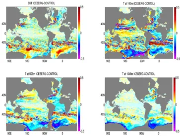
Figure 6.Changes in the global fields of salinity at selected depth levels (surface, 163, 508, 1046 m), averaged over years 26–30.
ORCA025 runs is realistic, although summer sea ice concen-trations are somewhat lower than in the data. Lower summer sea ice concentration in the Southern Ocean is a known bias in most forced models, and is attributed to regional uncer-tainties in the reanalysis fields (see discussion in Megann et al., 2014).
Icebergs substantially influence sea ice distribution, thick-ness and total mass. Changes are most evident in the SH. Figures 4 and 5 show year 26–30 means for ICEBERG, and differences relative to CONTROL, in southern hemispheric sea ice concentration and thickness. Including icebergs, con-centration and thickness are notably decreased at most loca-tions around Antarctica. In parts of the eastern Weddell Sea, concentration decreases by up to ∼20 % – e.g. at around
25◦W, 70◦S, concentration decreases from∼0.6 in
CON-TROL to∼0.5 in ICEBERG – with more limited increases,
of up to ∼10 % in the Bellingshausen Sea. At locations of
maximum thickness difference in the eastern Weddell and central Ross seas, annual-mean thicknesses of∼50–100 cm
in CONTROL are reduced by ∼10 cm in ICEBERG.
Con-versely, sea ice of thickness∼100 cm thickens by∼10 cm
throughout the Bellingshausen and Amundsen seas, as far as the eastern Ross Sea and along the western Antarctic Penin-sula.
Considering the combined effect of net reductions in annual-mean concentration and thickness in the SH, the total mass of sea ice (averaged over years 26–30) of 4.715×10¹⁵kg in CONTROL (ICEBERG) is decreased by
2.9 % in ICEBERG. Following the energy budget of MA10, we take the latent heat of fusion of water (334×103J kg−1), and consider a notional southern hemispheric sea ice area of 1013m2. The sea ice volume decrease in ICEBERG, in-terpreted as a consequence of differences in the annual cy-cle compared to CONTROL, thus equates to additional
en-Figure 7.As Fig. 6, for potential temperature.
ergy uptake of 0.14 W m−2, which is an order of magnitude smaller than the corresponding uptake in MA10.
Generally speaking, sea ice concentration and thickness are decreased (increased) in regions where surface salinity is higher (lower) in ICEBERG (see Sect. 3.3), consistent with sea ice formation responding to the strength of the halocline – a direct thermodynamic iceberg influence on sea ice. Local coincidence of changes of sea ice thickness and concentra-tion also suggests an indirect effect of icebergs on internal sea ice dynamics, in turn related to changes in upper ocean stratification. We infer that the presence of icebergs thus re-duces sea ice convergence in much of the Weddell and Ross seas. In the Bellingshausen and Amundsen seas, sea ice drift is westward (along shore) and divergent (e.g. Holland and Kwok, 2012). In these regions, icebergs thus appear to reduce the divergence of sea ice transport, conversely increasing ice thickness and concentration.
Decreased sea ice concentration and thickness in ICE-BERG is consistent with decreases at most affected grid points in the coupled atmosphere–ocean model of MA10. In the Greenland/Arctic area, the presence of icebergs leads to only minor re-distributions of sea ice concentration and thickness (not shown).
3.3 Impacts on hydrography
Figures 6 and 7 show ICEBERG differences, relative to CONTROL, in the global fields of salinity and potential tem-perature at selected depth levels (surface, 163, 508, 1046 m), averaged over years 26–30, thus accounting for short-term differences associated with transient eddies that are excited by icebergs. Given the relatively short experiments, an im-portant caveat is that differences are likely to be less equili-brated as depth increases.
Figure 8. Meridional transect along 35◦W, showing changes in salinity (upper panel) and temperature (lower panel), averaged over years 26–30.
Differences are strongly positive immediately adjacent to Antarctica (>0.2 psu at most longitudes), where runoff is substantially reduced (in proportion to the specified calving flux), but salinity differences also exceed 0.05 across broad swathes of the high-latitude Southern Ocean. Salinity in ICE-BERG is notably increased in regions where annual-mean sea ice concentration and thickness is strongly reduced (see Figs. 4 and 5). This suggests that differences in the seasonal cycle of sea ice freezing, export and melting contribute sub-stantially to the increases of surface salinity in ICEBERG.
Weaker negative differences are coincident with the lo-cally strong iceberg melting “plume” to the east of the Antarctica Peninsula, in the Atlantic sector of the Southern Ocean (see Fig. 3). More distinct negative differences are coincident with the highest concentration of Greenland ice-bergs, around Davis Strait. With increasing depth, negative differences are more evident in southern high latitudes, and are extensive throughout the Weddell Sea at 508 and 1046 m. Temperature differences are also substantial. At the sur-face, positive differences are extensive at southern high lat-itudes, again coincidental with differences in sea ice con-centration and thickness. A simple explanation is that sur-face temperatures are higher due to stronger sursur-face ocean heat gain where sea ice is thinner and/or absent for more
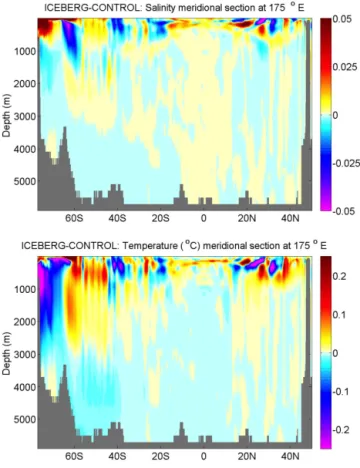
Figure 9.As Fig. 8, at 175◦E.
of the year. Large differences are also evident sub-surface, with widespread negative differences in the Atlantic and Pa-cific sectors of the high-latitude Southern Ocean. In the Wed-dell Sea, where particularly large negative differences extend to great depth (e.g.∼1000 m), we can conclude that a thin
warmer, more saline layer lies above an otherwise cooler, fresher water column. This implicit re-partitioning of heat and freshwater is associated with locally reduced sea ice con-centration and thickness.
Substantial salinity and temperature differences are also evident at lower latitudes, such as in the South Atlantic to at least∼500 m, with broader freshening and cooling of the
tropical and subtropical Atlantic at this depth. At all four se-lected depth levels, large salinity and temperature differences are also evident near strong currents such as the Antarctic Circumpolar Current, and western boundary currents such as the Gulf Stream and Kuroshio. We show in Sect. 3.5 that such differences are also associated with changes in ocean currents.
south-Figure 10.Area-averagedT/Sdiagrams representative of the Wed-dell Sea (50–70◦S, 15–55◦W; upper panel) and the Ross Sea (50– 70◦S, 172◦E–137◦W; lower panel), for ICEBERG (red points) and CONTROL (blue points).
ern latitudes. In the Weddell Sea of ICEBERG, negative dif-ferences of up to 0.01 psu – below 100–200 m – extend to around 2000 m. In Fig. 8, it is evident that Antarctic Interme-diate Water (AAIW) in ICEBERG is fresher by up to 0.01 (around 40◦S, 1300 m). This fresh signal may be traced back
to the region of iceberg melting east of the Antarctic Penin-sula, and may be a transient signal of locally more dominant iceberg melting earlier in the hindcast, noting that the pos-itive surface salinity differences progressively spread north-ward from the coastal zone of Antarctica over years 21–30 (not shown).
To show how temperature and salinity change in relation to density, for selected regions where iceberg influences are strongest, Fig. 10 shows area-averaged T–S (temperature– salinity) diagrams for the Ross Sea/Pacific and Weddell Sea/Atlantic sectors (both south of 50◦S, excluding all grid points near the coast). An overall impression (upper panels) is that ICEBERG salinities (red points) are mostly shifted to lower salinity below around 300 m, by up to 0.01 psu rel-ative to CONTROL salinities (blue points). Area-averaged differences are generally not temperature compensated at up-per levels (above∼500 m), leading to ICEBERG density
in-creases (shifts across isopycnals) on depth levels in the up-per 500 m, reaching maxima of∼0.015 kg m−3 at∼100 m
and∼0.030 kg m−3at 5 m, in the Weddell Sea and Ross Sea,
respectively. Below∼1000 m, changes of salinity and
tem-perature are very close to density compensating, although (a)
(b)
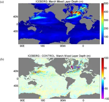
Figure 11. Mixed layer depth in March (year 26–30 average): (a)ICEBERG;(b)ICEBERG minus CONTROL.
there are, on average, slight density decreases in ICEBERG at around 4000 m in the Weddell Sea and at around 500 m in the Ross Sea. These density changes will potentially influ-ence dense water formation and the global abyssal circulation in a longer simulation.
Averaged over years 26–30, global volume-averaged salin-ity is 0.00025 psu higher in ICEBERG compared to CON-TROL, while for the Antarctic region (south of 50◦S),
volume-averaged salinity is 0.0015 psu higher in ICE-BERG. By contrast, in the North Atlantic (north of 50◦N)
volume-averaged salinity is around 0.0010 lower in ICE-BERG. These very small differences are within the inter-annual variations of global-mean and regional-mean salinity, and confirm that the prescribed freshwater fluxes in CON-TROL and ICEBERG are identical.
3.4 Impacts on mixed layer depth
Related to their widespread impact on the seasonal evolution of salinity and temperature, icebergs exert an influence on end-of-winter MLDs. Figures 11 and 12 show global fields of average March and September MLD, in ICEBERG and the difference from CONTROL, averaged over years 26–30. In March (Fig. 11), areas of greatest MLD (>500 m) in the North Atlantic are generally shallower in ICEBERG by up to 100 m (purple shading in Fig. 11b), notably in the cen-tral Labrador Sea, and in patches north and south of Ice-land. Conversely, in the western subtropics of the North Pa-cific, MLDs of up to 250 m in ICEBERG are in many places around 25 m deeper than in CONTROL.
(a)
(b)
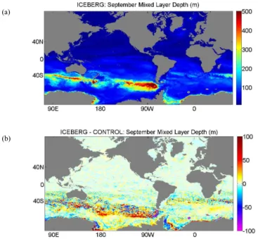
Figure 12.Mixed layer depth in September (year 26–30 average): (a)ICEBERG;(b)ICEBERG minus CONTROL.
icebergs. From 180◦E to around 90◦W, in the zone 50–
65◦S, ICEBERG MLDs in the range 200–400 m are
gen-erally deeper than those in CONTROL, by around 50 m at many locations. This can be related to hydrographic changes. North of∼60◦S in the Southern Ocean, we conjecture that
increased surface salinity in ICEBERG (see Fig. 6) is mostly driven by the weaker re-distribution of freshwater by sea ice, which is a first-order mechanism for transporting freshwa-ter northward in the Southern Ocean and contributes to the fresh signature of AAIW. In ICEBERG, reductions in sea ice concentration and thickness (Figs. 4 and 5) are indicative of reduced northward transport of (thinner) sea ice, with sea ice melting shifted southward. This appears to have a large im-pact on subducting AAIW properties (see Fig. 8) and local MLD, as outlined above. We also note substantial changes close to Antarctica, notably in the western sectors of the Weddell and Ross seas, where MLDs of 100–200 m in ICE-BERG are up to 50 m shallower than in CONTROL.
3.5 Impacts on ocean currents
To quantify the mean strength of ocean currents, we take the time average of kinetic energy (KE), here simply defined as (u2+v2)/2 whereuandv are the zonal and meridional components of the ocean current, at selected depths. The difference of KE is calculated from currents averaged over years 26–30 in ICEBERG relative to CONTROL (1KE), and shown in Fig. 13 at three levels, 61, 163 and 508 m (the deeper levels coincident with levels chosen to show property changes).
Starting in the region most directly impacted by re-partitioning of freshwater fluxes, we find negative
near-(a)
(b)
(c)
Figure 13. Differences (ICEBERG minus CONTROL) in the year 26–30 time average of kinetic energy (KE) at (a) 61 m; (b)163 m;(c)508 m.
surface 1KE values at all depths of the ACoC that skirts Antarctica, particularly in the Atlantic sector. This indicates a weaker baroclinic component of the ACoC in ICEBERG, due to changes in the cross-shelf density gradients (low to high density moving cross shelf) that drive an eastward flow com-ponent of the ACoC via the thermal wind balance (Núñez-Riboni and Fahrbach, 2009, 2010). The ACoC is a primarily wind-driven westward current (Hayakawa et al., 2012), so the thermal wind component in ICEBERG more strongly op-poses the largely unchanged westward component. We note that wind forcing can possibly increase with reduced sea ice concentration, but this effect is likely to be small. The stronger thermal wind would be consistent with particularly strong offshore cooling at, e.g. 163 and 508 m, indicated in Fig. 7.
More remote from Antarctica, we find high near-surface
(up to 0.05 m2s−2)– notably the Gulf Stream and Kuroshio currents. The substantial and coherent area of 1KE in the Kuroshio, persistent over the 5-year averaging period, cor-responds to an increase in the central meandering jet, and a decrease in the south part of this jet.
A more detailed view of the Gulf Stream region is pro-vided in Fig. S6 in the Supplement. The spatial structure of
1KE is coherent with depth, between the surface and 200– 300 m, but differences rapidly decline below 300 m. Temper-ature differences averaged over years 26–30 (see Fig. 7) are spatially coherent on large scales in the vicinity of bound-ary currents. For example, considering negative differences in excess of−0.5◦C, a substantial cold anomaly is apparent
to the north of the Gulf Stream at 508 m. We conclude here that property differences throughout the global ocean are to an extent associated with systematic changes in ocean cur-rents. In the relatively short simulations here, these remote changes (in properties and currents) must be excited by rapid propagation of density anomalies from high to low latitudes, a mechanism discussed briefly in Sect. 5.
4 Prototype modifications of NEMO–ICB
While we have focused so far on a baseline simulation with NEMO–ICB, three modifications of the iceberg model have been most recently implemented and are currently being tested in a slightly different ORCA025 configuration. These modifications will possibly be included in future code re-leases and are therefore only briefly described and discussed below.
4.1 Advection of icebergs with vertically integrated ocean velocity
Icebergs in the real world are influenced by the vertical shear of ocean currents. In particular, Ekman drift is suspected to affect iceberg trajectory. In a first modification of the base-line code, the depth-averaged ocean velocity is used in place of surface currents for advecting icebergs. In practice, the ocean velocity value used by the iceberg dynamics solver corresponds to the depth-averaged ocean velocity between the surface and the deepest tracer grid-point reached by the iceberg. Preliminary results suggest that iceberg trajectories are sensitive to this modification. Iceberg movements are lo-cally less erratic, being less affected by high-frequency fluc-tuations of surface currents and winds. The large-scale dis-tribution of icebergs, especially in the Southern Ocean, also appears to be affected by this modification.
4.2 Iceberg interaction with shallow bathymetry The thickness of bigger icebergs in the model is not negli-gible in comparison to the bathymetry of several coastal re-gions in the ORCA025 configuration. Is also known that big icebergs can get stuck on shallow bathymetry around
Antarc-tica, where they stay for long periods of time before moving northwards. Furthermore, using depth-integrated currents for advecting icebergs also requires accounting for how icebergs interact with shallow bathymetry (where depth-averaged cur-rents can be ill-defined). Fully accommodating this interac-tion with shallow bathymetry in the iceberg model could be complicated and computationally expensive. Indeed, in the model, Lagrangian particles represent a collection of ice-bergs with identical parameters, but physically we do not ex-pect the bathymetry to “stock” more than one iceberg at the same time. We therefore tested two simpler options for han-dling iceberg interaction with shallow bathymetry, although comparison with observations remains largely qualitative. These options are outlined as follows:
– Option A: shallow bathymetry points are considered as islands. With this modification, icebergs tend to travel around shallow regions, or eventually get stuck when no escape is possible, until melting enough to cross the shallow region.
– Option B: icebergs proceed across shallow bathymetry, even if their thickness exceeds the local depth. In this case, the iceberg drift velocity is computed from depth-averaged ocean currents (see Sect. 4.1), which now in-clude masked values (zero currents) at model depth lev-els below the seabed. With this choice, icebergs are slowed down over shallow bathymetry but can still tran-sit through shallow regions.
Preliminary results suggest that the differences between the two options appear not globally very important in the long term, but further work and longer simulations are needed. However, we see more remarkable differences of individual trajectories close to coastal areas.
4.3 Melting rates computed with the 3-D temperature field
To further resolve vertical physics in the model, we are also testing modifications for computing melting rates from the 3-D ocean temperature field. All three components of melt rate in the baseline version of ICB depend on surface tem-perature, and are reconsidered/modified accordingly:
– Basal melting: in our 3-D modification, we consider in-stead the temperature at the maximal depth reached for each iceberg.
– Buoyant convection at the sidewalls: this is a quadratic temperature-dependent function; in our 3-D modifica-tion, this function is integrated between the surface and the maximum depth of each iceberg.
In the few cases when icebergs are at a grid point where bathymetry is shallower than the iceberg thickness, the tem-perature considered for the part of iceberg that is deeper than bathymetry takes the value of the deepest ocean point.
Preliminary results show that, overall, this modification leads to a slightly higher global melt rate. In the Southern Ocean, this happens mostly during the boreal autumn and winter months (from April to September) when icebergs start transiting across the Weddell and Ross seas. Icebergs there-fore tend to melt faster which leads to shorter trajectories downstream in the northern Weddell and Ross seas. Inciden-tally, with 3-D temperature, icebergs are also less sensitive to some surface warm biases that may appear related to the stronger stratification induced by iceberg melting, but further analysis is required for more robust conclusions about this modification.
5 Summary and discussion
We have included icebergs interactively in an eddy-permitting global configuration of the ocean model NEMO, the first time that icebergs have been implemented at this resolution. Simulated iceberg distributions and freshwater fluxes are in reasonable agreement with limited available ob-servations, in the northwest Atlantic (Bigg et al., 2014a, and references therein) and in the Southern Ocean (Tournadre et al., 2012).
Freshwater forcing due to iceberg melting is most pro-nounced very locally, in the coastal zone around much of Antarctica, where it often exceeds in magnitude and opposes the negative freshwater fluxes associated with sea ice freez-ing. However, at most locations in the polar Southern Ocean, the annual-mean freshwater flux due to icebergs, if present, is typically an order of magnitude smaller than the contribution of sea ice and precipitation. A notable exception is the south-west Atlantic sector of the Southern Ocean, where iceberg melting reaches around 50 % of net precipitation over a large area. Including icebergs, sea ice concentration and thickness are notably decreased at most locations around Antarctica, by up to∼20 % in the eastern Weddell Sea, with more
lim-ited increases, of up to ∼10 %, in the Bellingshausen Sea.
Antarctic sea ice mass decreases by 2.9 %, overall.
As a consequence of changes in net freshwater forcing and sea ice, salinity and temperature distributions are also substantially altered. Surface salinity increases by∼0.1 psu around much of Antarctica, due to suppressed coastal runoff, with extensive freshening at depth, extending to greatest depths in the high-latitude Southern Ocean where discernible effects on both salinity and temperature reach 2500 m in the Weddell Sea by the last pentad of the simulation.
Our choice of reference run (CONTROL) has consider-able bearing on the present results. Most DRAKKAR simula-tions with ORCA025 now use static 2-D maps of freshwater flux due to melting icebergs. Further experiments and
analy-sis would be necessary to establish the impact of interactive icebergs on the model ocean, in contrast to implicit iceberg melting. A step in this direction is to preserve runoff rates around the ice sheets and ice caps. In a shorter sensitivity experiment, ICEBERG2, we re-ran the first 10 years of the hindcast with calved icebergs as in ICEBERG and runoff as in CONTROL. The icebergs in ICEBERG2 thus provide an additional freshwater flux, and the Southern Ocean (in par-ticular) consequently freshens almost everywhere. Such an experiment provides the preliminary basis for investigating the sensitivity of the ocean to ice sheet mass imbalance.
Coherent patterns of difference in salinity and tempera-ture develop throughout the global ocean, and ocean currents are systematically altered. Perturbations in the high-latitude density field, associated with icebergs, will propagate around the globe as Rossby and Kelvin waves. Previous model stud-ies have shown the importance of wave-like mechanisms for communication between Antarctic and equatorial regions (e.g. Atkinson et al., 2009). In such studies, salinity anoma-lies in the Southern Ocean excite fast westward-propagating barotropic planetary waves (Gill, 1982), which propagate to the western boundary of the South Pacific. On arrival at the western boundary, these Rossby waves excite baro-clinic Kelvin waves, which propagate more slowly to, and then along, the Equator. However, the perturbations applied in previous model studies were artificial, involving large and sustained changes in salinity over substantial portions of the Southern Ocean. In contrast to these studies, salinity and temperature differences between ICEBERG and CONTROL can be regarded as fluctuations that are more naturally associ-ated with melting icebergs. It is also possible for the density anomalies associated with iceberg melting to directly gener-ate baroclinic planetary waves, which can propaggener-ate similar distances, much more slowly, but with potentially larger am-plitude. In conclusion, more experiments for longer periods of time are needed to better understand slower variability of the system, and the various ocean teleconnections associated with variable iceberg calving and melting.
In the context of NEMO development and evaluation, the effects of icebergs on surface property fields and mixed layer depths (MLDs) are noteworthy. Megann et al. (2014) evalu-ate a similar 30-year hindcast using a global eddy-permitting configuration of NEMO v3.4. Over large areas of the world oceans, SST and surface salinity errors (Fig. 1 in Megann et al., 2014) exceed±0.25◦C and ±0.1 psu respectively, with
SST biases of±1.0◦C near Greenland. Based on the SST
hind-cast, the inclusion of icebergs may further improve realism in the subpolar North Atlantic, where we find reductions in end-of-winter MLDs of the order of 10 %.
The baseline representation of icebergs has been extended to represent iceberg interactions with shallow topography, and to use 3-D velocity and temperature fields to force ice-berg drift and melt. We are, however, not yet vertically re-solving the iceberg melting rates. Given that the size of our maximum iceberg is much less than even the ORCA025 res-olution, and that buoyant plumes from iceberg basal and side-wall melting are expected to rise quickly to the surface within a few hundred metres, applying these fluxes to the surface is inherently reasonable at current model resolutions. Large icebergs may exert a more remote influence on hydrography, at distances of up to several 10s of kilometres (Stephenson et al., 2011). Melting at sufficient depth may lead to the en-trainment and upwelling of relatively warm and salty Cir-cumpolar Deep Water around large icebergs in the South-ern Ocean (Jenkins, 1999). Stephenson et al. (2011) report observations of the corresponding alternative ways that ice meltwater disperses from a large tabular iceberg in the north-ern Weddell Sea: turbulent entrainment, localized near the iceberg, as well as wider horizontal dispersal due to double diffusive processes, as originally demonstrated in pioneering laboratory experiments (Huppert and Turner, 1980). Repre-sentation of large icebergs and these associated processes is currently beyond the capability of NEMO–ICB.
More feasible is the development of iceberg interaction with sea ice. At high sea ice concentration, icebergs tend to drift with the sea ice (Lighey and Hellmer, 2001). However, trajectories for individual giant icebergs (e.g. B31 over the austral winter of 2014 – see Bigg et al., 2014b) indicate that this only holds when the icebergs are frozen in to thick pack (essentially land-fast ice), rather than in the extensive areas where lead formation is common. More generally, we antic-ipate a maximum in the velocity of icebergs moved by sea ice, proportional to sea ice thickness and inversely propor-tional to iceberg draft (Morison and Goldberg, 2012). For sea ice moving at velocities higher than this maximum, sea ice ridging is expected, amounting to a dynamical feedback of icebergs on sea ice. In ongoing work, we have implemented solutions proposed by Hunke and Comeau (2011), and ini-tial findings are that iceberg trajectories are sensitive to these changes.
Finally, NEMO–ICB may be used with a parameteriza-tion of ice shelf cavity melting, to more realistically rep-resent rapidly changing mass fluxes from Antarctica to the surrounding ocean. This combined capability should under-pin experiments with enhanced calving and melting rates that eventually supplant current state-of-the-art protocols for freshwater forcing (van den Berk and Drijfhout, 2014). In the longer term, it would be desirable for ocean models with this capability to be included in future experimental activities of the Coupled Model Inter-comparison Project.
Code availability
NEMO–ICB is available via the NEMO home page, where new users can register via http://www.nemo-ocean. eu/user/register. Registered users can access the ICB modules at https://forge.ipsl.jussieu.fr/nemo/browser#trunk/ NEMOGCM/NEMO/OPA_SRC/ICB
ICB comprises the following modules:
– icb_oce.F90 – declares variables for iceberg tracking – icbclv.F90 – calving routines for iceberg calving – icbdia.F90 – initializes variables for iceberg budgets and
diagnostics
– icbdyn.F90 – time stepping routine for iceberg tracking – icbini.F90 – initializes variables for iceberg tracking – icblbc.F90 – routines to handle boundary exchanges for
icebergs
– icbrst.F90 – reads and writes iceberg restart files – icbstp.F90 – initializes variables for iceberg tracking – icbthm.F90 – thermodynamics routines for icebergs – icbtrj.F90 – trajectory I/O routines
– icbutl.F90 – various iceberg utility routines.
Default iceberg parameters are specified at https: //forge.ipsl.jussieu.fr/nemo/browser/trunk/NEMOGCM/ CONFIG/SHARED/namelist_ref
When compiling NEMO–ICB, the flag ln_icebergs in this namelist file is set to .true.
The Supplement related to this article is available online at doi:10.5194/gmd-8-1547-2015-supplement.
Acknowledgements. We thank Torge Martin and Alistair Adcroft for providing their code as a basis for the ICB module. Funding to couple NEMO with the icebergs module was provided by the UK Natural Environment Research Council (grant number NE/H021396/1) for the project “A century of variability in Greenland melting and iceberg calving”. We are grateful to three anonymous reviewers and the topic editor for a wide range of helpful comments and insights.
References
Atkinson, C. P., Wells, N. C., Blaker, A. T., Sinha, B., and Ivchenko, V. O.: Rapid ocean wave teleconnections linking Antarctic sea salinity anomalies to the equatorial ocean-atmosphere system, Geophys. Res. Lett., 36, L08603, doi:10.1029/2008GL036976, 2009.
Bigg, G. R. and Wadley, M. R.: Prediction of iceberg trajectories for the North Atlantic and Arctic Oceans, Geophys. Res. Lett., 23, 3587–3590, 1996.
Bigg, G. R., Wadley, M. R., Stevens, D. P., and Johnson, J. A.: Mod-elling dynamics and thermodynamics of icebergs, Cold Reg. Sci. Technol., 26, 113–135, 1997.
Bigg, G. R., Wei, H. L., Wilton, D. J., Zhao, Y., Billings, S. A., Hanna, E., and Kadirkamanathan, V.: A century of variation in the dependence of Greenland iceberg calving on ice sheet surface mass balance and regional climate change, P. R. Soc. A, 470, doi:10.1098/rspa.2013.0662, 2014a.
Bigg, G. R., Marsh, R., Wilton, D., and Ivchenko, V. O.: B31 – a giant iceberg in the Southern Ocean, Ocean Challenge, 20, 32– 34, 2014b.
Fichefet, T. and Maqueda, M. A.: Sensitivity of a global sea ice model to the treatment of ice thermodynamics and dynamics, J. Geophys. Res., 102, 12609–12646, 1997.
Gill, A. E.: Atmosphere-Ocean Dynamics, Academic Press, 662 pp., 1982.
Gladstone, R., Bigg, G. R., and Nicholls, K.: Iceberg trajectory modeling and meltwater injection in the Southern Ocean, J. Geo-phys. Res., 106, 19903–19915, 2001.
Hayakawa, H., Shibuya, K., Aoyama, Y., Nogi, Y., and Doi, K.: Ocean bottom pressure variability in the Antarctic Divergence Zone off Lützow-Holm Bay, East Antarctica, Deep-Sea Res. Pt. I, 60, 22–31, 2012.
Holland, P. R. and Kwok, R.: Wind-driven trends in Antarctic sea-ice drift, Nat. Geosci., 5, 872–875, doi:10.1038/ngeo1627, 2012. Hunke, E. C. and Comeau, D.: Sea ice and iceberg dy-namic interaction, J. Geophys. Res., 116, C05008, doi:10.1029/2010JC006588, 2011.
Hunke, E. C. and Lipscomb, W. H.: CICE: The Los Alamos Sea Ice Model, Documentation and Software User’s Manual, Ver-sion 4.1, Tech. Rep. LA-CC-06-012, Los Alamos National Lab-oratory, Los Alamos, New Mexico, available at: http://oceans11. lanl.gov/trac/CICE (last access: 13 May 2015), 2010.
Huppert, H. E. and Turner, J. S.: Ice blocks melting into a salinity gradient, J. Fluid. Mech., 100, 367–384, 1980.
Jenkins, A.: The impact of melting ice on ocean waters, J. Phys. Ocean., 29, 2370–2381, 1999.
Jongma, J. I., Driesschaert, E., Fichefet, T., Goosse, H., and Renssen, H.: The effect of dynamic–thermodynamic icebergs on the Southern Ocean climate in a three-dimensional model, Ocean Model., 26, 104–113, 2009.
Levine, R. C. and Bigg, G. R.: The sensitivity of the glacial ocean to Heinrich events from different sources, as modeled by a cou-pled atmosphere-iceberg-ocean model, Paleoceanography, 23, PA4213, doi:10.1029/2008PA001613, 2008.
Lighey, C. and Hellmer, H. H.: Modeling giant-iceberg drift under the influence of sea ice in the Weddell Sea, Antarctica, J. Glaciol., 47, 452–460, 2001.
Madec, G.: “NEMO ocean engine”. Note du Pole de modélisation, Institut Pierre-Simon Laplace (IPSL), France, No. 27 ISSN No 1288-1619, 2008.
Marsh, R., Ivchenko, V. O., Skliris, N., Alderson, S., Bigg, G. R., Madec, G., Blaker, A., and Aksenov, Y.: NEMO-ICB (v1.0): in-teractive icebergs in the NEMO ocean model globally configured at coarse and eddy-permitting resolution, Geosci. Model Dev. Discuss., 7, 5661–5698, doi:10.5194/gmdd-7-5661-2014, 2014. Martin, T. and Adcroft, A.: Parameterizing the fresh-water flux from
land ice to ocean with interactive icebergs in a coupled climate model, Ocean Model., 34, 111–124, 2010.
Megann, A., Storkey, D., Aksenov, Y., Alderson, S., Calvert, D., Graham, T., Hyder, P., Siddorn, J., and Sinha, B.: GO5.0: the joint NERC-Met Office NEMO global ocean model for use in coupled and forced applications, Geosci. Model Dev., 7, 1069– 1092, doi:10.5194/gmd-7-1069-2014, 2014.
Morison, J. and Goldberg, D.: A brief study of the force balance between a small iceberg, the ocean, sea ice, and atmosphere in the Weddell Sea, Cold Reg. Sci. Technol., 76–77, 69–76, 2012. Núñez-Riboni, I. and Fahrbach, E.: Seasonal variability of
the Antarctic Coastal Current and its driving mechanisms in the Weddell Sea, Deep-Sea Res. Pt. I, 56, 1927–1941, doi:10.1016/j.dsr.2009.06.005, 2009.
Núñez-Riboni, I. and Fahrbach, E.: An observation of the banded structure of the Antarctic Coastal Current at the prime meridian, Polar Res., 29, 322–329, doi:10.1111/j.1751-8369.2010.00166.x, 2010.
Rayner, N. A., Parker, D. E., Horton, E. B., Folland, C. K., Alexan-der, L. V., Rowell, D. P., Kent, E. C., and Kaplan, A.: Global analyses of sea surface temperature, sea ice, and night marine air temperature since the late nineteenth century, J. Geophys. Res., 108, 4407, doi:10.1029/2002JD002670, 2003.
Rignot, E., Velicogna, I., van der Broeke, M. R., Monaghan, A., and Lenaerts, J.: Acceleration of the contribution of the Greenland and Antarctic ice sheets to sea level rise. Geophys. Res. Lett., 38, L05503, doi:10.1029/2011GL046583, 2011.
Silva, T. A. M., Bigg, G. R., and Nicholls, K. W.: The contribu-tion of giant icebergs to the Southern Ocean freshwater flux, J. Geophys. Res., 111, C03004, doi:10.1029/2004JC002843, 2006. Stephenson, G. R., Sprintall, J., Gille, S. T., Vernet, M., Helly, J. J., Kaufmann, R. S.: Subsurface melting of a free-floating Antarctic iceberg, Deep-Sea Res. Pt. II, 58, 1336–1345, doi:10.1016/j.dsr2.2010.11.009, 2011.
Tournadre, J., Girard-Ardhuin, F., and Legrésy, B.: Antarctic ice-bergs distributions, 2002–2010, J. Geophys. Res., 117, C05004, doi:10.1029/2011JC007441, 2012.
van den Berk, J. and Drijfhout, S. S.: A realistic freshwater forcing protocol for ocean-coupled climate models, Ocean Model., 81, 36–48, doi:10.1016/j.ocemod.2014.07.003, 2014.
Watkins, S. J., Maher, B. A., and Bigg, G. R.: Ocean circu-lation at the Last Glacial Maximum: a combined modelling and magnetic proxy-based study, Paleoceanogr., 22, PA2204, doi:10.1029/2006PA001281, 2007.