Image Compression Using Moving Average Histogram and RBF Network

Image Compression Using Moving Average Histogram and

RBF Network

SANDER ALI KHOWAJA*, AND IMDAD ALI ISMAILI* RECEIVED ON 13.02.2015 ACCEPTED ON 17.03.2015

ABSTRACT

Modernization and Globalization have made the multimedia technology as one of the fastest growing field in recent times but optimal use of bandwidth and storage has been one of the topics which attract the research community to work on. Considering that images have a lion’s share in multimedia communication, efficient image compression technique has become the basic need for optimal use of bandwidth and space. This paper proposes a novel method for image compression based on fusion of moving average histogram and RBF (Radial Basis Function). Proposed technique employs the concept of reducing color intensity levels using moving average histogram technique followed by the correction of color intensity levels using RBF networks at reconstruction phase. Existing methods have used low resolution images for the testing purpose but the proposed method has been tested on various image resolutions to have a clear assessment of the said technique. The proposed method have been tested on 35 images with varying resolution and have been compared with the existing algorithms in terms of CR (Compression Ratio), MSE (Mean Square Error), PSNR (Peak Signal to Noise Ratio), computational complexity. The outcome shows that the proposed methodology is a better trade off technique in terms of compression ratio, PSNR which determines the quality of the image and computational complexity.

Key Words: Image Compression, Histogram Averaging, Radial Basis Function, Compression Ratio, Peak Signal to Noise Ratio, Computational Complexity.

* Institute of Information & Communication Technology, University of Sindh, Jamshoro.

expressive which can determine the personality and interests of a user, people having high resolution cameras in their smart phones prefer to use image content, rising popularity of visual social networks etc. Increase in the image content increases the need of bandwidth for multimedia communication. Bandwidth is a costly resource indeed which encourage the researchers to work on better image compression techniques i.e. keeping the visual quality of the image same while reducing the storage size with a reasonable execution time.

1.

INTRODUCTION

self-The process of compressing the image refers to the reduction of image size in such a way that after reconstruction the image should look the same as original image or to be precise it should look exactly like original image. If the reconstructed image is an exact replica of the original image as determined by the evaluating parameters i.e. MSE and PSNR then the compression algorithm can be classified as lossless otherwise it will be classified as lossy [1]. Use of compression algorithm can fulfill the need of saving channel bandwidth and storage capacity therefore the choice of compression algorithm depends on the application specificity and user tolerance. Lossy compression technique can provide greater compression ratios by compromising the quality of the image and on the contrary lossless compression can provide lower compression ratios while keeping the visual quality almost the same [2].

There are numerous applications which can tolerate the loss of information bits, loss of quality, change of dimension etc. while using lossy compression techniques but some applications prefer high quality over high compressed file as they cannot stack the loss of information which includes medical images, satellite images, surveillance of high security zone, GIS and remote sensing images [2]. These applications cannot risk the original information in image but can compromise on lower compression ratios as slight change in information can change the whole analysis.

The use of neural network have been increased in image compression algorithms due to their flexibility and architecture, infact what makes the neural network intrinsically robust is the non-usage of entropy coding hence making it a decent choice for communication having noisy channel [3-5]. Implementing neural networks demands a trade-off in terms of computational complexity as it takes a lot of time during training phase but use of neural networks i.e. Radial basis function in the proposed method is somewhat different, in this method we created

our own database of 100 images with varying resolutions and used this database for training the network model, training is particularly performed on the color data sets so the weights obtained by the training are saved for further use. The reason for performing this particular task is to reduce the computational complexity of the system, as the weights have already been provided so the execution time will be the fraction of what training time takes. The employment of neural networks is responsible for making the compression technique lossless thus the visual quality of the image remains same. There are benefits of using neural networks but at the same time there are some drawbacks associated with it which is discussed in the conclusion section, however experimental results show that the proposed method yields very impressive results without compromising on image quality and resolution with better trade-off in terms of CR and PSNR as compared to the existing algorithms.

Later part of this paper is organized as follows. Section 2 will provide “State of the art” information for image compression methods and neural networks followed by a review of previous work in Section 3. Section 4 explains the proposed methodology for implementing the said technique. Section 5 provides the results after employing the said technique for image compression and evaluation of this method in terms of compression ratio, PSNR, MSE and computation complexity have also been carried out in this section and, finally we will conclude it in Section 6.

2.

STATE OF THE ART

2.1

Image Compression Methods

transformations suggesting that the transformation is reversible, hence the data can be recovered. This type of technique can be classified as statistically redundant and the compression is said to be lossless compression. On the other end visually extraneous method suggests that the data which is irrelevant in terms of visual quality can be removed to compress an image, this type of transformation cannot be reversed hence classified as lossy compression. It is obvious that if we can tolerate the loss of information we can go for visually extraneous methods as it achieves higher compression ratios but this paper focuses on achieving the high compression ratios using statistically redundant methods, consequently attaining the goal of lossless compression in true means. Following are the different models of compression that can be used for classical image compression methods.

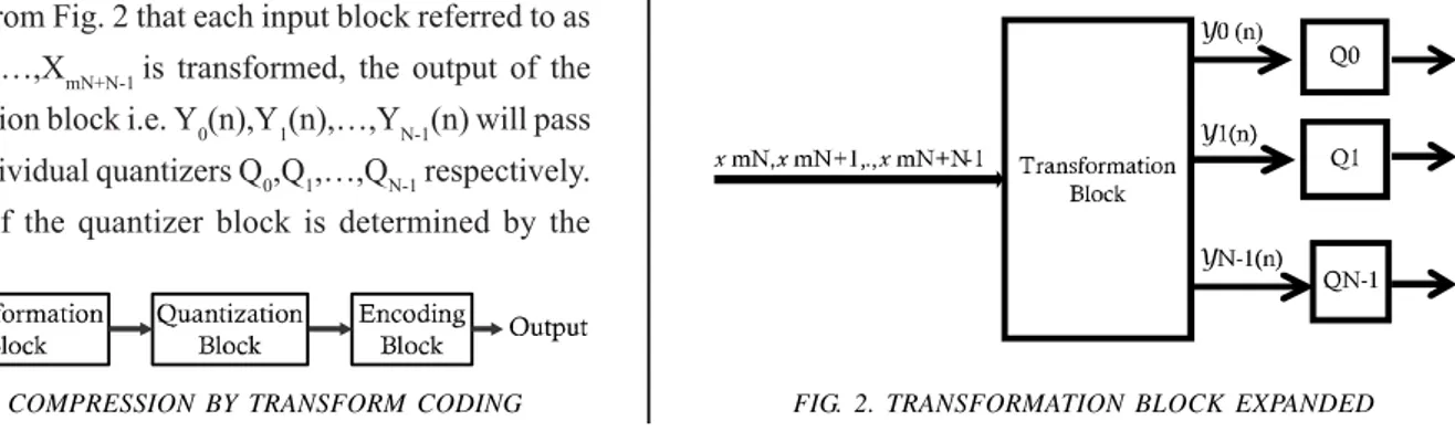
Transform Coding: Most widely used method in the field of image compression [6], Fig. 1 depicts the working of this technique. This method acquires the images and process it using transformation block followed by the process of quantization and finally encoding is performed which actually compresses the image, however the compression performed by the encoder can be reversed back i.e. lossless compression but the losses are incurred in quantizer block which performs the alteration of bits.

Transformation block is responsible for transforming the pixels of an image into bits or in the form understandable by the quantizer and encoder. The process performed by the transformation block is illustrated in Fig. 2.

It is clear from Fig. 2 that each input block referred to as X_mN, X_mN+1,…,X_mN+N-1 is transformed, the output of the transformation block i.e. Y₀(n),Y₁(n),…,Y_N-1(n) will pass through individual quantizers Q₀,Q₁,…,Q_N-1 respectively. Selection of the quantizer block is determined by the

process of bit-allocation, quantizers are connected with their particular encoders which map the symbols in binary digits but now modern systems analyze multiple quantized values before applying entropy to the whole bit stream. Similarly the color images are processed using transform coding by considering each color as a monochrome set of pixels followed by the same mechanism. One of the most popular method for such type of transformation is DCT (Discrete Cosine Transform) [1,7], another widely used transformation technique is wavelet transform [8].

Predictive Coding: Another image compression technique

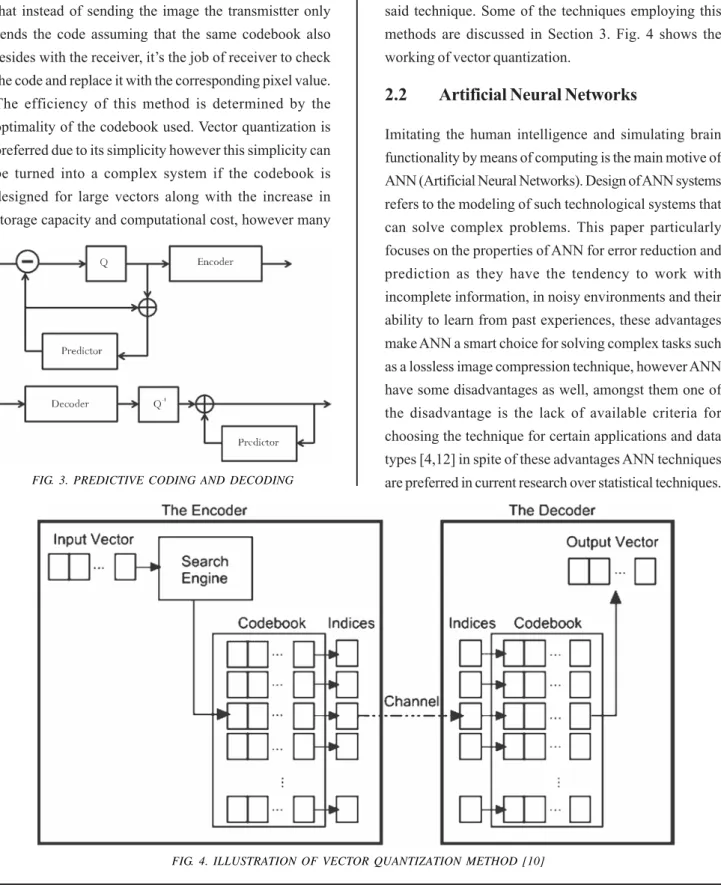
which predicts the next value of pixels by calculating the prediction error [9], quantized and coded data values are the reflection of this prediction error. Predictive coding works in a very similar fashion as of differential PCM systems where the past values are taken into account and the value of actual pixel is predicted based on the prediction error, decoder predicts the value in a similar way along with the integration of error fetched from the predicted values to recover the original signal. In order to perform a feedback loop some synchronization mechanism is need to be employed, working of predictive coding is illustrated in Fig. 3. The complexity in this method lies with the design of predictor which demands the design of a statistical model which can relate the neighboring pixels with the original ones. Autoregressive model can be used as a predictive coding technique.

Vector Quantization: Vector quantization technique

proposes a design of model containing the information of

pixel patterns in the form of a codebook which represents each pixel pattern with a unique index [10-11], suggesting that instead of sending the image the transmistter only sends the code assuming that the same codebook also resides with the receiver, it’s the job of receiver to check the code and replace it with the corresponding pixel value. The efficiency of this method is determined by the optimality of the codebook used. Vector quantization is preferred due to its simplicity however this simplicity can be turned into a complex system if the codebook is designed for large vectors along with the increase in storage capacity and computational cost, however many

techniques in fusion with vector quantization have been proposed to reduce the computational complexity of the said technique. Some of the techniques employing this methods are discussed in Section 3. Fig. 4 shows the working of vector quantization.

2.2

Artificial Neural Networks

Imitating the human intelligence and simulating brain functionality by means of computing is the main motive of ANN (Artificial Neural Networks). Design of ANN systems refers to the modeling of such technological systems that can solve complex problems. This paper particularly focuses on the properties of ANN for error reduction and prediction as they have the tendency to work with incomplete information, in noisy environments and their ability to learn from past experiences, these advantages make ANN a smart choice for solving complex tasks such as a lossless image compression technique, however ANN have some disadvantages as well, amongst them one of the disadvantage is the lack of available criteria for choosing the technique for certain applications and data types [4,12] in spite of these advantages ANN techniques are preferred in current research over statistical techniques. FIG. 3. PREDICTIVE CODING AND DECODING

As our preferred ANN technique used in the proposed method is Radial Basis Function, this part will present the review on RBF networks.

Error Back Propagation Method: This method uses

supervised learning to reduce or predict the error and is used by Multilayer feed forward networks, this network uses log-sigmoid and tangent hyperbolic as their activation function [13]. The characteristic of this network is it calculates the error at the output of each layer to employ numerical methods for reducing the error. The adjustment of the weights is done by back propagating the results from the output of each layer, this is a recursive process for achieving the desired goal.

The idea of error back propagation was derived from steepest descent gradient method but in order to overcome the limitations associated with the said technique error back propagation also employs conjugate gradient alogrithm or levenberg marqardt method [14] to optimize the error, radial basis function resides under the category of error back propagation method. Fig. 5 shows simple network architecture of error back propagation method comprising of input layer, hidden layer and output layer respectively, in Fig. 5 the nodes can only be connected to nodes in forward layer hence the name multilayer feedforward networks, the connections in Fig. 5 refers to the synaptic weights and nodes are referred as neurons.

Radial Basis Function Network: RBF networks uses error

back propagation method for error reduction and classification purposes, due to its radially bounded nature and use of symmetrical transfer functions RBF networks can also give an impression of general regression or probabilistic networks. Unlike MLP (Multilayer Perceptron) which is the most popular technique in ANN domain this paper prefers the use of RBF networks as it overcomes one of the limitations of MLP i.e. Local minima problem and converges fast than MLP networks [13].

The main characteristic of radial basis function is their feature of increasing and decreasing monotonically with respect to the center due to the use of Gaussian function, the computation i.e. the error reduction in RBF networks is based on three parameters namely: shape of the function, the center and the distance between input and center. This relation is mathematically expressed in Equation (1).

(

)

⎟

⎟

⎠

⎞

⎜

⎜

⎝

⎛

−

= ₂

width 2 centre n

Y(n) ₍₁₎

The proposed technique uses exact fitting method of RBF networks using exact neuron fitting calculations, this could be referred to as exact interpolation method suggesting that in order to find the output function h(J) the input vector J_i should be projected on the desired target M_i, can be mathematically expressed as:

M_i = h(J_i), where i = 1,….,n (2)

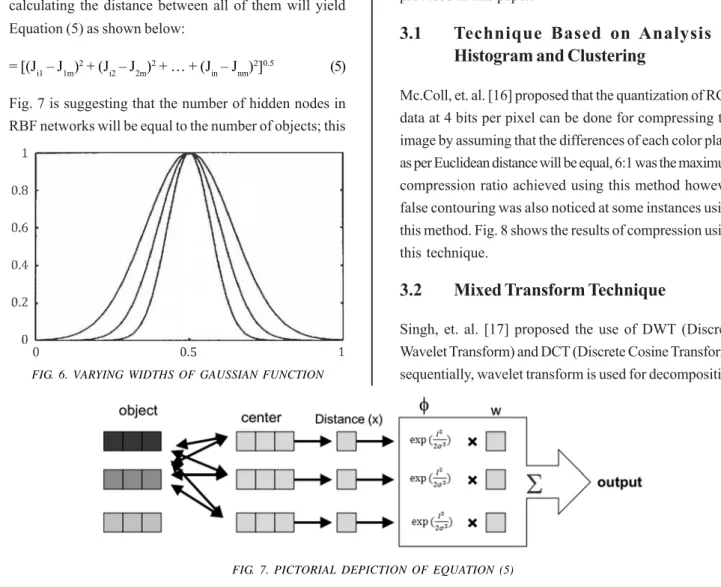
In Equation (2) n is the number of objects, for exact mapping approach it is necessary to use basis functions for every data point or we can say that n basis functions will be used by using the function φ(||j_i - j_m||), where φ(.) and

|| ||refers to function and Euclidean distance between J_i and J_m respectively [38]. The output of this function in terms of linear mapping can be shown in Equation (3):

(

)

x : 1

m W_n J_i J_m

) i

h(J =_{∑ =} φ − ₍₃₎

Where J_i and J_mis the input and center function respectively and W_m is the weight for this function however the RBF uses Gaussian function so replacing the input value in in equation 1 we will get the expression shown in Equation (4):

(

)

⎟⎟

⎟

⎠

⎞

⎜⎜

⎜

⎝

⎛

− =

− ₂

2σ 2 m J i J exp m J i J

φ ₍₄₎

σ2 in Equation (4) defines the smoothness parameter of

the Gaussian function for interpolation, the varying widths of Gaussian function is shown in Fig. 6.

Considering that we have n number of inputs so calculating the distance between all of them will yield Equation (5) as shown below:

= [(J_i1 – J_1m)2 _{+ (J}

i2 – J2m)2 + … + (Jin – Jnm)2]0.5 (5)

Fig. 7 is suggesting that the number of hidden nodes in RBF networks will be equal to the number of objects; this

is the main idea behind exact fitting method in RBF networks.

3.

EXISTING APPROACHES FOR

IMAGE COMPRESSION

Several researchers around the globe have contributed a lot to this field for development of efficient compression mechanism with a better trade off technique in terms of compression ratio and quality of an image, as a sophisticated algorithm can magnanimously save the storage space required for saving high definition images [15]. Since image compression field is quite mature the available literature is very dense, consolidation of a limited work based on good results and better trade-offs is provided in this paper.

3.1

Technique Based on Analysis of

Histogram and Clustering

Mc.Coll, et. al. [16] proposed that the quantization of RGB data at 4 bits per pixel can be done for compressing the image by assuming that the differences of each color plane as per Euclidean distance will be equal, 6:1 was the maximum compression ratio achieved using this method however false contouring was also noticed at some instances using this method. Fig. 8 shows the results of compression using this technique.

3.2

Mixed Transform Technique

Singh, et. al. [17] proposed the use of DWT (Discrete Wavelet Transform) and DCT (Discrete Cosine Transform) sequentially, wavelet transform is used for decomposition FIG. 6. VARYING WIDTHS OF GAUSSIAN FUNCTION

of coefficients followed by vector quantization for coding the values and discrete cosine transform will be used for extraction of low frequency components from the coded values, results proposed by this method are shown in Table 1.

3.3

Fractal Coding

Koli, et. al. [18] suggesting that RGB plane should be individually extracted and compressing the image by applying the fractal coding to each of the color plane. Compression ratio of approximately 16:1was achieved using this method. Fig. 9 shows the result using this particular method.

3.4

DWT and VQ Based Image Compression

Debnath, et. al. [19] proposed a compression method by using discrete wavelet transform for decomposing each image in three levels and then dividing them into 10 separate sub bands for coding using vector quantization method. Results from the said technique are shown in Fig. 10.

3.5

ACO, GA and PSO Based Image

Compression

Uma, et. al. [20], suggested that the results obtained by fractal coding can further be optimized by using the swarm intelligence techniques such as Particle Swarm Optimization, Ant Colony Optimization and Genetic

Algorithms to enhance the quality of the image and to reduce the computational cost of fractal coding technique. Results fetched from this technique are shown in Table 2.

3.6

Machine Learning Techniques

Zhang, et. al. [2], proposed machine learning technique i.e. MLP (Multilayer Perceptron) for prediction of color patterns based on semi-supervised learning, prediction of colors using machine learning methods will result in compressed image as shown in Fig. 11.

3.7

Partition K-Means Clustering using

Hybrid DCT-VQ

Mahapatra, et. al. [21], proposed the use of discrete cosine transform as energy compaction technique to reduce the

. o

N Method PSNR CR Resulst

.

1 JPEG 20.7 67:1 Marginal d

e s o p o r

P 30.7 67:1 AlmotsPefrect

.

2 JPEG 27.6 60:1 Poor

d e s o p o r

P 30.8 60:1 Good

.

3 JPEGs 27.1 67:1 Marginal d

e s o p o r

P 31.2 67:1 AlmotsPefrect

.

4 JPEG 29.4 68:1 Good

d e s o p o r

P 29.3 68:1 AlmotsPefrect

TABLE 1. COMPARISON OF MIXED TRANSFORM WITH JPEG [17]

computational cost of codebook generated by vector quantization to speed up the process. The result is not much qualitative in terms of PSNR but compression ratio was increased to approximately 21:1.

3.8

Lifting Based Wavelet Transform

Coupled with SPIHT

Kabir, et. al. [22], specifically proposed the compression technique for medical images by using wavelet transform technique coupled with SPIHT (Set Partition in Hierarchal Trees) coding algorithm to overcome the limitations of compression based on solely wavelet transform methods, result of image using this technique is shown in Fig. 12.

3.9

Embedded Techniques with Huffman

Coding

Srikanth, et. al. [23], proposed a method which combines Huffman coding with wavelet transform based methods to increase the compression ratio with some increased computational complexity at the decoder while reconstructing the image, result of this method can be visualized in Fig. 13.

f o s e p y T

m h ti r o g l

A RangeBlocksComRpariteosnison EnTciomdeing PSNR(dB) A

G 4x48x8 6.73:1 2370 26.22

O S

P 4x48x8 13:1 347 24.43

O C

A 4x48x8 1.89:1 6500 3439

TABLE 2. PERFORMANCE MEASURE OF ACO, PSO AND GA ALGORITHM [20]

FIG. 9. ORIGINAL AND COMPRESSED IMAGES USING FRACTAL CODING [18]

on the literature mentioned in this section Table 3 have been compiled showing the maximum PSNR achieved using these particular methods

4.

PROPOSED METHODOLOGY

This paper proposes an image compression method based

on moving average histogram followed by RBF networks for providing better image quality than existing methods and a better trade-off in terms of CR, computational complexity with enhanced quality. Fig. 14 depicts the working of the proposed methodology which involves four stages i.e.

FIG. 11. ORIGINAL AND COMPRESSED IMAGES USING MACHINE LEARNING [2]

FIG. 12. ORIGINAL AND COMPRESSED IMAGE USING WT & SPIHT [22]

„

„

„

„

4.1

Pre-Processing Stage

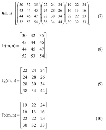
This stage deals with the acquisition of input image and making the input image compatible for further processing, the proposed system can apply on multiple image formats e.g. JPEG, GIF, PNG, TIFF etc. This stage sub-divides a color image in four planes i.e. Black & White (BW Image), Red color image, Blue color image and Green color image as shown in Fig. 15. Assuming that the input image is J(m,n) the representation can be represented in the mathematical form as written in Equation (6).

J(m,n) = [Jr(m,n), Jg(m,n), Jb(m,n)] (6)

. o

N CompresisonTechnique _PM_SNax_Rim₍u_dm_B)

.

1 Hitsogram_TeA_cn_ha_nl_iy_qs_usi_e&_16]Clutseirng NA

.

2 MixedTransformTechnique[17] 31.2

.

3 FractalCoding[18] 27.24

.

4 VQwtihWaveeltTransform[19] 38.17

.

5 GA,PSO&ACOTechnique[20] 34.39

.

6 K-meansC_Dlu_Cts_Te_-ir_Vng_Qba_[2se₁d_]onHybird 30.44

.

7 Machine elarningtechnique[22] 34.1

.

8 WaveeltT_Sra_Pn_Is_Hfo_Trm_[2c₂o_]upeldwtih 50.01

.

9 SeamCarvin_Dg_efo_vr_cieA_srb_[2irt₄a_]ryResoluiton 45.58

. 0

1 Embedde_Hd_uc_ffo_mm_ap_nre_Cs_ois_do_in_ngte_[c₂h₃n_]iquewtih 36.7

TABLE 3. LITERATURE SURVEY OF COMPRESSION TECHNIQUES [2,16-24]

Where J(m,n) is an input image separately represented in Red, Green and Blue color in form of Jr(m,n), Jg(m,n), Jb(m,n) respectively, it can be further explained by considering an example shown in Equation (7).

⎥ ⎥ ⎥ ⎥ ⎦ ⎤ ⎢ ⎢ ⎢ ⎢ ⎣ ⎡ ⎟ ⎟ ⎟ ⎟ ⎠ ⎞ ⎜ ⎜ ⎜ ⎜ ⎝ ⎛ ⎟ ⎟ ⎟ ⎟ ⎠ ⎞ ⎜ ⎜ ⎜ ⎜ ⎝ ⎛ ⎟ ⎟ ⎟ ⎟ ⎠ ⎞ ⎜ ⎜ ⎜ ⎜ ⎝ ⎛ = 33 32 30 23 22 22 16 13 16 24 22 19 , 44 34 38 34 30 28 26 28 24 24 24 22 , 54 53 52 47 45 44 45 44 43 35 32 30 n) J(m, (7)

⎥

⎥

⎥

⎥

⎦

⎤

⎢

⎢

⎢

⎢

⎣

⎡

⎥

⎥

⎥

⎥

⎦

⎤

⎢

⎢

⎢

⎢

⎣

⎡

⎥

⎥

⎥

⎥

⎦

⎤

⎢

⎢

⎢

⎢

⎣

⎡

Equations (8-10) represents the extraction of Red, Green and Blue color matrices from the input matrix shown in Equation (7), however, the extraction of black and white image is performed by using Local binary pattern

suggesting that a mean of the input matrix is calculated and assigned as a threshold, every pixel of an image is then compared with this threshold for returning the logical values of 1 and 0, mathematically this process can be written as shown in Equation (11).

⎩

⎨

⎧

Illustration of these equations in graphical format can be visualized in Fig. 15.

4.2

Processing Stage

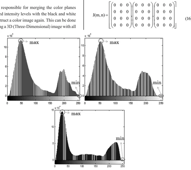
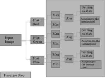
This is the stage which actually performs the compression as the moving average histogram is employed at this stage which is responsible for the reduction of color intensity levels, moving average histogram takes into account each of the color matrix separately as shown in Fig. 16.

Moving average histogram as shown in Fig. 16 selects the maximum and minimum level of each histogram and calculates the average separately, this average value is then assigned to the first pixel and again the process continues for taking the average of maximum and minimum values and assign it to the respective pixel, if at any stage the maximum value gets equal to the minimum value then all of the remaining pixels will be assigned the minimum value. Its mathematic representation is shown in Equations (12-15).

Max = max [Jr(m,n)] (12)

Min = min [Jr(m,n)] (13)

2 Min Max n)

Avg(m, = + (14)

Jr(m,n) = Avg(m,n) (15)

Where m=0,1,2,…,i-1 and n=0,1,2,…,j-1 suggesting that i and j are the number of pixels in rows and columns respectively, these equations only refer to the calculation performed on Red matrix, similarly the same calculations will be performed on green and blue matrices and pixel values will be updated in a cyclic fashion. Graphical representation of this algorithm is shown in Fig. 17.

4.3

Combining Stage

This stage is responsible for merging the color planes having reduced intensity levels with the black and white image to construct a color image again. This can be done by first creating a 3D (Three-Dimensional) image with all

zeros in it but of the same dimension as of the BW image and other color planes, second step is to replace the logical values of BW image in the dummy matrix created and replicate it for all three matrices, third step is to replace all ones by 255 and all zeros will remain same. By applying this method we can convert the BW 2D image into 3D but still this is not the image what we desire as still the values are not the ones which have been calculated using moving average histogram but we have made the image compatible for merging of reduced color intensity levels in the original BW image. Final step of this stage is to convolve each corresponding matrices for replacement of reduced color intensity levels in the 3D image created using BW image. Mathematical representation of this stage is explained through Equations (16-22).

⎥

⎥

⎥

⎥

⎦

⎤

⎢

⎢

⎢

⎢

⎣

⎡

⎟

⎟

⎟

⎟

⎠

⎞

⎜

⎜

⎜

⎜

⎝

⎛

⎟

⎟

⎟

⎟

⎠

⎞

⎜

⎜

⎜

⎜

⎝

⎛

⎟

⎟

⎟

⎟

⎠

⎞

⎜

⎜

⎜

⎜

⎝

⎛

⎩

⎨

⎧

=

Otherwise 0

1 n) BW(m, 255

:,1)

J(:, ₍₁₇₎

⎩

⎨

⎧

=

Otherwise 0

1 n) BW(m, 255

:,2)

J(:, ₍₁₈₎

⎩

⎨

⎧

=

Otherwise 0

1 n) BW(m, 255

:,3)

J(:, ₍₁₉₎

J(:,:,1) * Jr(m,n) = J(:,:,1) (20) J(:,:,2) * Jg(m,n) = J(:,:,,2) (21) J(:,:,3) * Jb(m,n) = J(:,:,3) (22)

The series of equation will merge the reduced color intensity levels with BW image values to reconstruct the original image i.e. J(m,n) but with errors as this will be the

compressed image. Graphical interpretation of these equations can be seen in Fig. 18.

4.4

Error Minimization Stage

This is the final stage of the proposed algorithm where the reconstructed image is provided as an input to the RBF networks for reducing the error and making the image qualitative. The mathematical explanation of RBF networks has been already carried in ANN (Artificial Neural Network) study a sub-section in Section 2. However, its graphical representation is shown in Fig. 19 and the result of passing the image through this stage is shown in Fig. 20 for better understanding of the proposed algorithm.

4.5

Evaluation Parameters

For evaluating the proposed method and validating the results a comparison is carried out with the existing methods on the basis of following parameters.

„

„

„

5.

RESULTS

The proposed method have been tested on 35 images with varying resolutions and have been compared with the results of existing methods used for image compression technique, comparison is based on FIG. 17. MOVING AVERAGE HISTOGRAM METHOD

evaluation metrics to validate the results. Simulations are carried out using MATLAB, proposed method have been evaluated in terms of visual quality, based on Peak signal to noise ratio and compression ratio along with the computational complexity.

5.1

Evaluation Based on Visual Quality

There are 35 images which have been tested using the proposed method, as the images are large in volume some of the results obtained by simulating the said algorithm has been shown in Figs. 21-24 and can be analyzed from the resultant images that there is negligible or no difference in terms of visual quality of the images.

5.2

Evaluation Based on PSNR and CR

Table 4 shows the results obtained by simulating the proposed method, evaluation in Table 4 has been carried out with respect to MSE, PSNR and CR.

The results shown in Table 4 have not only been applied to low resolution images but it has been tested to varying resolution for high definition images as well with almost the same PSNR as the existing methods proposed but with better trade-offs with respect to the compression ratios. Table 5 provides the comparison between existing methods with the proposed method in terms of PSNR and CR.

It can be analyzed from Table 5 that the proposed method offers the best trade-off in terms of CR and quality of the image; however, the proposed method outperforms other existing methods if the comparison is based solely on PSNR.

5.3

Evaluation Based on Computational

Complexity

Image compression is a mature field in terms of research but still a very few research work mentions the time complexity for their methods, Table 6 is compiled for the available literature based on computational complexity for the methods used in image compression technique but all the existing methods are tested on low resolution images so the comparison is based on image resolution of 512x512 image for the validity of assessment being carried out.

FIG. 19. METHODOLOGY CARRIED OUT IN ERROR-MINIMIZATION STAGE

FIG. 22(a). ORIGINAL IMAGE

(COURTESY: GOOGLE IMAGES) FIG. 22(b). COMPRESSED IMAGE

FIG. 23(a). ORIGINAL IMAGE

(COURTESY: GOOGLE IMAGES) FIG. 23(b). COMPRESSED IMAGE FIG. 21(a). ORIGINAL IMAGE

(COURTESY: GOOGLE IMAGES)

FIG. 24(a). ORIGINAL IMAGE (COURTESY: GOOGLE IMAGES)

FIG. 21(b). COMPRESSED IMAGE

. o

N ImageResoluiton OirginalFielSzie CompressedFielSzie CR MSE PSNR(dB) .

1 150x150 28KB 2.44KB 11.47 2.793 43.67

.

2 256x256 156KB 10KB 15.6 3.43 42.77

.

3 347x346 184KB 12.2KB 15.08 2.03 45.06

.

4 385x276 88KB 8.6KB 10.23 1.615 46.05

.

5 414x415 104KB 16.2KB 6.42 0.66 49.92

.

6 512x512 136KB 15.9KB 8.55 1.0379 47.97

.

7 512x512 404KB 32.9KB 12.28 3.829 42.80

.

8 512x512 460KB 45.5KB 10.11 1.24 47.20

.

9 612x459 472KB 38.2KB 12.36 4.027 42.08

. 0

1 693x693 440KB 60.8KB 7.24 4.3 41.80

. 1

1 768x768 1.08MB 131KB 8.44 4.289 41.98

. 2

1 768x768 372KB 20.9KB 17.8 0.478 51.33

. 3

1 800x635 784KB 50.3KB 15.59 0.4706 51.40

. 4

1 864x1152 1.42MB 141KB 10.31 1.554 46.22

. 5

1 1024x768 1.03MB 67.5KB 15.62 1.911 45.31

. 6

1 1024x768 1.32MB 61.7KB 21.91 3.44 42.76

. 7

1 1024x768 960KB 78.8KB 12.18 2.176 44.75

. 8

1 1152x864 1.81MB 212KB 8.74 1.475 46.44

. 9

1 1280x1024 2.07MB 212KB 9.99 5.11 41.34

. 0

2 1536x2048 4.09MB 292KB 14.34 1.642 45.97

. 1

2 1536x2048 3.35MB 378KB 9.07 1.342 46.85

. 2

2 1600x1214 1.63MB 180KB 9.27 0.6603 49.93

. 3

2 1680x1050 3.66MB 296KB 12.66 6.25 40.17

. 4

2 1680x1050 2.94MB 273KB 11.03 5.811 40.48

. 5

2 1920x1080 3.5MB 354KB 10.12 7.706 39.26

. 6

2 1920x1080 3.76MB 353KB 10.91 4.32 41.78

. 7

2 1920x1080 4.17MB 359KB 11.89 16.6 35.92

. 8

2 1920x1200 5.81MB 456KB 13.05 1.337 46.87

. 9

2 1920x1200 4.76MB 397KB 12.28 6.852 39.77

. 0

3 1920x1440 3.31MB 307KB 11.04 3.154 43.14

. 1

3 1944x2592 7.39MB 702KB 11.57 3.36 42.86

. 2

3 2048x1536 4.28MB 404KB 10.84 2.36 44.39

. 3

3 2448x3264 10.1MB 1.11MB 9.09 1.62 46.03

. 4

3 2448x3264 13.1MB 1.44MB 9.1 2.509 44.13

. 5

3 5184x3888 23.6MB 1.79MB 13.18 1.30 46.99

5.4

Limitations

The limitation of this method is associated with the execution time while performing compression with the said technique, due to the employment of ANN in the proposed technique the execution time increases as the image resolution increases, however the execution time is still lower than many techniques. Results shown in Table 4 shows that the maximum image resolution tested was 5184x3888 but for compressing this particular image resolution the method consumes 32400 seconds which is not appropriate for practical use though up to the resolution of 2448x3264 the execution time is linear with respect to the result shown in Table 6.

. o

N Method MaximumCR MaximumPSNR(dB)

.

1 HitsogramAnalyssi&ClutseirngTechnique[16] 6 NA

.

2 MixedTransform[17] 60 30.80

.

3 FractalCoding[25] N.A 27.24

.

4 FractalCodingwtihdifferentdomain&ranges[18] 15.93 32.45

.

5 Fractalcodingwtihsprialarchtiecture[26] 11.22 31.26

.

6 DsicreteWaveeltTransform&VectorQuantziaiton[19] 22.66 38.17

.

7 AntColonyOpitmziaiton,_AP_la_gotr_rci_tihel_mS_sw_[2a₀rm_] Opitmziaiton&Genetci 13 34.39

.

8 Machine elarningtechnique[2] 23.7 34.1

.

9 ParititonK-meansclutseirngwtihHybirdDCT-VQ[21] 21.57 30.44

. 0

1 Lfiitngbasedwaveelt rtansformcoupeldwtihSPIHT[22] N.A 50.01

. 1

1 SeamCravingforArbirtaryDsipalyDevcies[24] N.A 45.58

. 2

1 EmbeddedTechniqueswtihHuffmanCoding[23] N.A 36.07

. 3

1 MulitwaveeltTransformCoding[27] 6.30 NA

. 4

1 SingualrValueDecompoisitonandWaveeltDifferenceReduciton[30] 20 42.06

. 5

1 JPEG2000[30] 20 41.05

. 6

1 WaveeltDifferenceReduciton[30] 20 37.76

. 7

1 ProposedMethodology 21.91 51.40

TABLE 5. COMPARISON OF EXISTING METHODS WITH PROPOSED TECHNIQUE

6.

CONCLUSION

this technique which refers to the computational complexity when image resolution increases but this method can be a basis for conducting the research to overcome this limitation in future. This method can be applied to number of applications including medical imaging, satellite imaging, Surveillance, military applications etc. where quality is a non-compromising factor and the computational time can be negotiated with. Results from this paper also concludes that there is still room for the improvement in achieving lossless image compression which makes the field of research still worthy for conducting further research.

ACKNOWLEDGEMENT

The first author has produced this paper from his Master of Engineering Project at the Institute of Information & Communication Technologies, Mehran University of Engineering & Technology, Jamshoro, Pakistan. The second author was his Co-Supervisor.

REFERENCES

[1] Ismaili, I.A., Khowaja, S.A., and Soomro, W.J. , “Image Compression, Comparison betweem Discrete Cosine Transform and Fast Fourier Transform and the problems associated with DCT”, International Conference on Image Processing, Computer Vision & Pattern Recognition, pp. 962-965, July, 2013.

[2] Zhang, C., and He, X., “Image Compression by Learning to Minimize the Total Error”, IEEE Transactions on Circuits and Systems for Video Technology, Volume 23, No. 4, April, 2013.

[3] Benbenisti, Y., Kornreich, D., Mitchell, H.B., and Schaefer, P., “Normalization Techniques in Neural Networ Image Compression”, Signal Processing: Image Communication, Volume 10, pp. 269-278, 1997.

[4] Khowaja, S.A., Shah, S.Z.S., and Memon, M.U. , “Noise Reduction Technique for images using Radial Basis Function Neural Networks”, Mehran University Research Journal of Engineering & Technology, Volume 33, No. 3, pp. 278-285, Jamshoro, Pakistan, July, 2014.

[5] Abbas, H.M., and Fahmy, M.M., “Neural Model for Karhunen-Loeve Transform with application to Adaptive Image Compression”, IEE Proceedings on Communications, Speech and Vision, Volume 140, No. 2, pp. 135-143, April, 1993.

[6] Li, D., and Loew, M., “Closed-Form Quality Measures for Compressed Medical Images: Statistical Preliminaries for Transform Coding”, Proceedings of IEEE 25th _Annual International Conference on Engineering in Medicine and Biology Society, Volume 1, pp. 837-840, September, 2003.

[7] Monro, D.M., and Sherlock, B.G., “Optimal Quantization Strategy for DCT Image Compression”, IEE Proceedings on Vision, Image and Signal Processing, Volume 143, No. 1, pp. 10-14, February, 1996.

[8] DeVore, R.A., Jawerth, B., and Lucier, B.J., “Image Compression through Wavelet Transform Coding”, IEEE Transactions on Information Theory, Volume 38, No. 2, pp. 719-746, March, 1992.

. o

N Method _TE_ix_me_ecu_(sit_eo_cn₎

.

1 GenetciAlgortihms[20] 2370

.

2 PatrcielSwarmOpitmziaiton[20] 347

.

3 AntColonyOpitmziaiton[20] 6500

.

4 FractalCoding[18] 1360800

.

5 WaveeltTransform[28] 6

.

6 ConvenitonalVectorQuantziaiton[19] 47.87

.

7 DsicreteWaveeltTransform[19] 18

.

8 K-meansClutseirng[21] 28

.

9 3-DSprialJPEG[28] 36

. 0

1 HybirdDCT-VQ[21] 19.21

. 1

1 PirncipelComponentAnalyssi[28] >100

. 2

1 Levenberg_MarquardtMethod[14] 4065.172

. 3

1 ModfieidLevenberg-MarquardtMethod[14] 2376.734

. 4

1 ProposedMethod 32.872

[9] Jiang, J., Edirisinghe, E.A., and Schroder, H., “A Novel Predictive Coding Algorithm for 3D Image Compression”, IEEE Transactions on Consumer Electronics, Volume 43, No. 3, pp. 430-437, August, 1997.

[10] Nasrabadi, N.M., and King, R.A., “Image Coding using Vector Quantization: A Review”, IEEE Transactions on Communication, Volume 36, pp. 84-95, August, 1988. [11] Gray, R.M. , “Vector Quantization”, IEEE ASSP

Magazine, Volume 1, pp. 4-29, 1984.

[12] Karayiannis, N.B., and Weigun, G.M. , “Growing Radial Basis Function Neural Networks: Merging Supervised and Un-Supervised Learning with Network Growth Techniques”, IEEE Transactions on Neural Networks, Volume 8, No. 6, pp. 1492-1505, 1997.

[13] Kenue, S.K.. “Modified Back Propagation Neural Network Applications to Image Processing”, Proceedings SPIE, Application of Artificial Neural Networks-III, Volume 1709, pp. 394-407, Orlando, Florida, April, 1992.

[14] Karthikeyan, P., and Sreekumar, N., “A Study on Image Compression with Neural Networks using Modified Levenberg-Marquardt Method”, Global Journal of Computer Science and Technology, Volume 11, No. 3, March, 2011.

[15] Shukla, J., Alwani, M., and Tiwari, A.K. , “A Survey on Lossless Image Compression Methods”, 2nd _{International} Conference on Computer Engineering & Technology, Volume 6, pp. 136-141, April, 2010.

[16] McColl, R.W., and Martin, G.R., “Compression of Color Image Data using Histogram Analysis and Clustering Technique”, Electronics & Communication Engineering Journal, Volume 1, No. 2, pp. 93-100, March, 1989.

[17] Singh, I., Agathoklis, P., and Antoniou, A., “Compression of Color Images using Mixed Transform Techniques”, IEEE Pacific Rim Conference on Communications, Computers and Signal Processing, Volume 1, pp. 334-337, August, 1997.

[18] Koli, N.A., and Ali, M.S., “Lossy Color Image Compression Technique using Fractal Coding with Different Size of Range and Domain Blocks”, International Conference on Advance Computing and Communications, pp. 236-239, December, 2006.

[19] Debnath, J.K., Rahim, N.M.S., and Fung, W.K., “A Modified Vector Quantization Based Image Compression Technique using Wavelet Transform”, IEEE International Joint Conference on Neural Networks, pp. 171-176, June, 2008.

[20] Uma, K., Palanisamy, P.G., and Poornachandran, P.G., “Comparison of Image Compression using GA, ACO and PSO Techniques”, International Conference on Recent Trends in Information Technology, pp. 815-820, June, 2011

[21] Mahapatra, D.K., and Jena, U.R., “Partition K-Means Clustering Based Hybrid DCT-Vector Quantization for Image Compression”, IEEE Conference on Information and Communication Technologies, pp. 1175-1179, April, 2013.

[22] Kabir, M.A., Khan, A.M., Islam, M.T., Hossain, M.L., and Mitul, A.F., “Image Compression using Lifting Based Wavelet Transform coupled with SPIHT Algorithm”, International Conference on Informatics, Electronics & Vision, pp. 1-4, May, 2013.

[23] Srikanth, S., and Meher, S., “Compression Efficiency for Combining Different Embedded Image Compression Techniques with Huffman Encoding”, International Conference on Communications and Signal Processing, pp. 816-820, April, 2013.

[24] Salma, E., and Kumar, J.P.J., “Efficient Image Compression based on Seam Craving for Arbitrary Resolution Display Devices”, International Conference on Communications and Signal Processing, pp. 529-532, April, 2013.

[25] Ghosh, S.K., and Mukherjee, J., “Novel Fractal Technique for Color Image Compression”, Proceedings of IEEE First Indian Annual Conference on INDICON, pp. 170-173, December, 2004.

[27] Rajakumar, K., and.Arivoli, T., “Implementation of Multi Wavelet Transform Coding for Lossless Image Compression”, International Conference on Information Communication and Embedded Systems, pp. 634-637, Februar, 2013.

[28] Wu, X., Hu, S., Tang, Z., Li, J., and Zhao, J., “Comparisons of Threshold EZW and SPIHT Wavelets Based Image Compression Methods”, TELKOMNIKA Indonesian Journal of Electrical Engineering, Volume 12, No. 3, pp. 1895-1905, March, 2014.

[29] Khowaja, S.A., “Neural Network Based Image Compression Technique by Reducing Color Intensity Levels”, Mehran University of Engineering & Technology, Thesis and Dissertations, May, 2014.