Comparison of automatic segmentation of full polarimetric SAR sea ice images with manually drawn ice charts

(1)

TCD

7, 2595–2634, 2013

Comparison of automatic and manual sea ice charts

M.-A. N. Moen et al.

Title Page

Abstract Introduction

Conclusions References

Tables Figures

◭ ◮

Back Close

Full Screen / Esc

Printer-friendly Version Interactive Discussion

Discussion

P

a

per

|

Di

scussion

P

a

per

|

Discussion

P

a

per

|

Discussi

on

P

a

per

|

The Cryosphere Discuss., 7, 2595–2634, 2013 www.the-cryosphere-discuss.net/7/2595/2013/ doi:10.5194/tcd-7-2595-2013

Geoscientiic Geoscientiic

Open Access

The Cryosphere Discussions

This discussion paper is/has been under review for the journal The Cryosphere (TC). Please refer to the corresponding final paper in TC if available.

Comparison of automatic segmentation of

full polarimetric SAR sea ice images with

manually drawn ice charts

M.-A. N. Moen1, A. P. Doulgeris1, S. N. Anfinsen1, A. H. H. Renner2, N. Hughes3, S. Gerland2, and T. Eltoft1,4

1

Department of Physics and Technology, University of Tromsø, 9037 Tromsø, Norway 2

Norwegian Polar Institute, FRAM Centre, 9296 Tromsø, Norway 3

Norwegian Ice Service, Norwegian Meteorological Institute, 9293 Tromsø, Norway 4

Northern Research Institute, 9294 Tromsø, Norway

Received: 22 May 2013 – Accepted: 27 May 2013 – Published: 13 June 2013

Correspondence to: M.-A. N. Moen (mari-ann.moen@uit.no)

(2)

TCD

7, 2595–2634, 2013

Title Page

Tables Figures

◭ ◮

Back Close

Full Screen / Esc

Discussion

P

a

per

|

Di

scussion

P

a

per

|

Discussion

P

a

per

|

Discussi

on

P

a

per

|

Abstract

In this paper we investigate the performance of an algorithm for automatic segmenta-tion of full polarimetric, synthetic aperture radar (SAR) sea ice scenes. The algorithm uses statistical and polarimetric properties of the backscattered radar signals to seg-ment the SAR image into a specified number of classes. This number was determined 5

in advance from visual inspection of the SAR image and by available in-situ measure-ments. The segmentation result was then compared to ice charts drawn by ice service analysts. The comparison revealed big discrepancies between the charts of the ana-lysts, and between the manual and the automatic segmentations. In the succeeding analysis, the automatic segmentation chart was labeled into ice types by sea ice ex-10

perts, and the SAR features used in the segmentation were interpreted in terms of physical sea ice properties.

Studies of automatic and robust estimation of the number of ice classes in SAR sea ice scenes will be highly relevant for future work.

1 Introduction

15

The Arctic ice cover has changed significantly during the last decades. The amount of multi-year ice has decreased and the general thinning of the ice cover supports the predictions that the Arctic will soon become dominated by first-year ice (Kwok et al., 2009; Maslanik et al., 2011). As a consequence of this development, shipping and exploration activity in ice infested Arctic areas have increased. Some human activities 20

in polar areas are crucially dependent on precise and reliable sea ice maps. Such maps are also important for environmental monitoring and global climate change studies. Hence, studies of seasonal variations in sea ice properties and coverage have become increasingly important.

At present, synthetic aperture radar (SAR) is one of the most important remote sen-25

(3)

TCD

7, 2595–2634, 2013

Title Page

Tables Figures

◭ ◮

Back Close

Full Screen / Esc

Discussion

P

a

per

|

Di

scussion

P

a

per

|

Discussion

P

a

per

|

Discussi

on

P

a

per

|

hostile climate and the remoteness limit the availability of in-situ data (Clausi and Deng, 2004). A SAR imaging sensor, which operates in the microwave frequency band, pro-vides all-weather and day-night high-resolution imagery. Recent radar sensors have polarimetric capabilities. A full-polarimetric SAR system transmits and receives both linear horizontal (H) and vertical (V) polarized electromagnetic waves, and hence pro-5

vides measurements in four polarization channels (quad-pol). These are referred to as the HH, VV, HV and VH channels. The HH and VV channels are often referred to as the co-polarization (co-pol) terms because the transmit and receive polarization is the same. The HV and VH terms are known as the cross-polarization (cross-pol) terms, as they relate to orthogonal polarization states. With full polarimetric capability, a SAR 10

system is able to distinguish di_fferent scattering types, such as surface, volume and double-bounce scattering.

Quad-pol scenes can be acquired at very high resolution. The Radarsat-2 scene analyzed in this paper has a spatial resolution of 4.7 m (slant range)_×4.9 m (azimuth) and covers an area of 25 km_×25 km.

15

Dual-pol scenes are images consisting of two polarimetric channels, such as HH and HV or VV and VH. These are preferred in operational ice charting services because of their much wider aerial coverage. Radarsat-2 ScanSAR Wide scenes have a coverage of 500 km_×500 km with 50 m resolution.

Despite the currently very limited coverage, the detailed quad-pol images are crucial 20

in order to understand the underlying physics of SAR imaging of sea ice. Investigation of full-polarimetric images will also contribute to an improved understanding of possi-bilities and limitations of single-pol and dual-pol images and helps select the optimal channel combinations.

The Canadian Ice Service (CIS) alone process ten to twelve thousand SAR images 25

(4)

classifica-TCD

7, 2595–2634, 2013

Title Page

Tables Figures

◭ ◮

Back Close

Full Screen / Esc

Discussion

P

a

per

|

Di

scussion

P

a

per

|

Discussion

P

a

per

|

Discussi

on

P

a

per

|

tion algorithm that is operational at present (B. Duguay, personal communication, 2013, and F. Dinessen, personal communication, 2013). Hence, there is a need to improve automatic segmentation and classification approaches to ice charting and monitoring (Clausi and Deng, 2004; Ochilov and Clausi, 2010; Kwon et al., 2013; Zakhvatkina et al., 2013). However, the Norwegian Ice Service offers more frequently updated auto-5

matic ice concentration maps, but these maps are experimental (F. Dinessen, personal communication, 2013). For automatic products see: http://polarview.met.no/.

There is not much work published on the validation of manual ice classification charts or on pixel-to-pixel comparisons between manual charts and automatic segmentations. Due to lack of ground truth, manual ice charts are considered the best available sea ice 10

information and thus often used for validation of automatic generated datasets (Clausi and Deng, 2004; Yu and Clausi, 2008; Ochilov and Clausi, 2010; Breivik et al., 2012; Kwon et al., 2013). Some information about validation of ice concentration maps is reported in Breivik et al. (2012).

Several techniques for automatic segmentation of SAR sea ice scenes exist. The ap-15

proaches include thresholding of polarimetric features (Scheuchl et al., 2001; Dierking et al., 2003; Geldsetzer and Yackel, 2009), use of gamma distribution mixture models (Samadani, 1995), K-means clustering (Hartigan, 1975; Karvonen, 2010), neural net-works (Hara et al., 1995; Karvonen, 2004; Bogdanov et al., 2005; Zakhvatkina et al., 2013), Markov random field models (Deng and Clausi, 2005), Gaussian mixture mod-20

els (Karvonen, 2004) and the Wishart classifier (Scheuchl et al., 2002, 2003). Gill and Yackel (2012) explored the classification potential of various SAR polarimetric param-eters using supervised classifications. The iterative region growing using semantics (IRGS) method, which combines edge-based and region-growing-based segmentation methods, is generally considered the state-of-the-art approach (Yu and Clausi, 2008; 25

Ochilov and Clausi, 2010; Clausi et al., 2010).

(5)

TCD

7, 2595–2634, 2013

Title Page

Tables Figures

◭ ◮

Back Close

Full Screen / Esc

Discussion

P

a

per

|

Di

scussion

P

a

per

|

Discussion

P

a

per

|

Discussi

on

P

a

per

|

and automatic segmentation results obtained by an automatic algorithm. In particular we seek answers to the following questions:

1. How well do manually generated and automatically generated segmentation maps match?

2. Can polarimetric parameters improve the separation between different ice types? 5

3. Can a physical interpretation of polarimetric features be exploited to label seg-ments found by the automatic algorithm?

One of the polarimetric parameters utilized in the segmentation, the relative kurtosis, has not been used in sea ice classification previously.

10

In this study we present results from data aquired during a field cruise to the edge of the Arctic Basin, north of Svalbard, in April 2011.

This paper is organized as follows: Section 2 describes the data set, satellite data and in-situ measurements analysed in this study. In Sect. 3 we explain how the manual and the automatic segmentation are produced and how the intercomparisons between 15

them are performed. The analysis of the data and the findings are presented in Sect. 4. The results are discussed in Sect. 5 and conclusions are given in Sect. 6.

2 Data

2.1 Satellite data

The satellite images were aquired by Radarsat-2, which is the second Canadian C-20

(6)

TCD

7, 2595–2634, 2013

Title Page

Tables Figures

◭ ◮

Back Close

Full Screen / Esc

Discussion

P

a

per

|

Di

scussion

P

a

per

|

Discussion

P

a

per

|

Discussi

on

P

a

per

|

year drifting sea ice at various stages of development and open and refrozen leads. This study focuses on a fine quad-pol scene aquired on 12 April 2011 at an incidence angle of 40◦. The scene is located north of Svalbard (Fig. 1). A Pauli colour coded representation (Lee and Pottier, 2009) of the scene is shown in Fig. 2a. That is, the po-larimetric intensity channel combinations_|HH−VV_|, 2_|HV_|and_|HH+VV_|are assigned 5

to the RGB channels, respectively. Three major scattering mechanisms can be visually differentiated by inspecting a Pauli image. Single bounce scattering, such as scattering from a surface appears bluish and the intensity depends on the roughness and orienta-tion to the radar. That is, a smooth surface will reflect most of the power away from the radar sensor, unless it is directly oriented towards the sensor, while rougher surfaces 10

have a significant di_ffuse backscatter at greater angles. Dihedral corners, like build-ings or water/ice edges, causes double-bounce scattering which appears red/purple in the Pauli representation. The green colour represents depolarisation, often as a re-sult of multiple random scattering from within the volume of the material. This type of scattering occurs in multiyear ice because its low salinity allows for penetration of the 15

electromagnetic (EM) waves into the ice where internal air bubbles and brine inclusions give multiple random reflections of the signal.

The 12 April dataset includes a broad collection of in-situ data. The time-lag between the satellite overpass and the start and end of a series of helicopterborne sea ice thickness measurements was 37 min and 1 h and 46 min, respectively. The relatively 20

short time span allows for an accurate sea ice drift correction.

2.2 In-situ measurements

The collection of in-situ measurements from 12 April 2011 comprises measurements of total thickness (snow plus ice thickness) retrieved during a helicopter flight, positions from different global positioning system (GPS) trackers, the bridge based sea ice ob-25

(7)

TCD

7, 2595–2634, 2013

Title Page

Tables Figures

◭ ◮

Back Close

Full Screen / Esc

Discussion

P

a

per

|

Di

scussion

P

a

per

|

Discussion

P

a

per

|

Discussi

on

P

a

per

|

image (see Fig. 2a). We include here a short introduction to sea ice thickness mea-surements using the EM-bird. More details can be found in Haas et al. (2009).

The large difference in conductivity between sea water and sea ice makes it possible to measure sea ice thickness by EM induction. The instrument induces an EM-field at the ice/water interface. The field strength and phase are used to calculate the distance 5

between the instrument and the bottom of the sea ice. The distance from the EM-bird to the air-ice interface, or air/snow interface in the case of snow-covered sea ice, is provided by a laser altimeter mounted on the EM-bird. The differences between these two measured distances is the total thickness within the footprint of the EM-bird (_∼40– 50 m) (Renner et al., 2013). The ice and snow thickness distribution derived from the 10

EM-bird measurements on 12 April 2011 is shown in Fig. 3.

Optical images from a camera (GoPro, model YHDC5170) were also aquired during these flights. The camera was mounted on the helicopter’s chassis, looking downwards onto the ice, and aquiring images at a frequency of 0.5 Hz. An Iridium Surface Velocity Profiler (ISVP) buoy was deployed onto an ice floe on 11 April 2011. Every hour the 15

buoy transmitted its position together with other parameters. The positions can be used to calculate the ice drift in the buoy’s vicinity. A GPS transmitter (Garmin DC-40 collar) was placed on the ice to track the ice drift occuring between and during the EM-Bird flight and satellite image aquisition. The GPS receiver (Garmin Astro 220 with Astro portable long range antenna) onboard the ship received the collar positions every 30 s 20

on average. The ice drift during the timespan of 1 h and 46 min was significant. We chose to compute the average ice drift during the EM-bird flight based on the Garmin Astro GPS due to the higher frequency of GPS-positions. The displacement of each thickness measurement was calculated based on its time-lag to the satellite image aquisition time and the average drift velocity. Figure 2a shows a Pauli image annotated 25

(8)

TCD

7, 2595–2634, 2013

Title Page

Tables Figures

◭ ◮

Back Close

Full Screen / Esc

Discussion

P

a

per

|

Di

scussion

P

a

per

|

Discussion

P

a

per

|

Discussi

on

P

a

per

|

3 Method

In this section we present the methods used for the preparation of the manual ice charts and the automatic segmentation of the SAR data. We also give a physical interpretation of the features used in the automatic algorithm. The last part of this section describes the intercomparison of the hand drawn ice maps and the automated segmentation. 5

3.1 Manual segmentation and classification

The Norwegian Ice Service’s operational ice charts are manually drawn based on dual-pol ScanSAR Wide data and available optical data. The charts are usually ice concen-tration maps, since the users are mainly interested in the ice edge and areas where it is possible to navigate into the ice.

10

The 12 April quad-pol scene was manually and independently segmented and clas-sified by two ice analysts at the Norwegian Ice Service. The analysts were instructed to concentrate on determining the ice stage of development (SoD) and the ice type. The colours used in the ice maps are those defined for standard World Meteorological Organization (WMO) stage of development ice charts (MANICE, 2005, chapt. 5.5.4) 15

with the addition of class 17 for frost-flower covered nilas. The authors would like to stress that the ice analysts have less experience in using quad-pol SAR scenes for ice type classification, and ice SoD charts are not produced for operational use. More infor-mation about operational manually drawn ice charts can be found in MANICE, (2005), pp. 146.

20

The scene was presented to the analysts as both radar backscatter coefficientσ0

in a colour composite (RGB) constructed from the VV, HV and HH channels, and as a Pauli decomposition (Fig. 2a). In addition, they were allowed to refer to the shipboard ice log and photographs from the NoCGV Svalbard. Areas observed by eye to be of similar appearance in the backscatter and Pauli image were masked out by using the 25

(9)

TCD

7, 2595–2634, 2013

Title Page

Tables Figures

◭ ◮

Back Close

Full Screen / Esc

Discussion

P

a

per

|

Di

scussion

P

a

per

|

Discussion

P

a

per

|

Discussi

on

P

a

per

|

permits an ice type attribute to be applied to each polygon. This is used to determine the colouring of the final ice map.

3.2 The automatic segmentation

In this section we will explain how the features used in the automatic segmentation are extracted. Those readers who are not familiar with radar images may skip to Sect. 3.3 5

without any contextual loss.

From a quad-pol SAR instrument, the complex scattering coefficients for all possible combinations of transmit and receive polarization are obtained. The scattering coeffi -cientsS_{i j},i,j_{∈ {}H,V_}are subscripted with the associated receive and transmit polari-sation. From the original scattering vector,s₌_[_S_HH_,_S_HV_,_S_VH_,_S_VV_]T_{, we calculated the}

10

reduced scattering vector, s_red₌_[_S_HH_,_√1

2(SHV+SVH),SVV]

T

, by assuming reciprocity

(SHV≃SVH). The operator ( )

T

defines the ordinary transpose operation, and the factor

1

√

2 ensures that the averaged cross-pol term preserves the power contained in the

in-dividual original cross-pol terms. In the following the scattering vectors are the reduced three-dimensional vectors with dimensiond=3.

15

The covariance matrix, given by Eq. (1), is calculated by averaging overL number

of scattering vectors. In this study,L=21×21=441. The averaging is done by using a stepping window.

C= 1

L L

X

i=1

s_isH

i (1)

where 20

C= 



hSHHSHH∗ i hSHHSHV∗ i hSHHSVV∗ i hSHVSHH∗ i hSHVSHV∗ i hSHVSVV∗ i hSVVSHH∗ i hSVVSHV∗ i hSVVSVV∗ i



(10)

TCD

7, 2595–2634, 2013

Title Page

Tables Figures

◭ ◮

Back Close

Full Screen / Esc

Discussion

P

a

per

|

Di

scussion

P

a

per

|

Discussion

P

a

per

|

Discussi

on

P

a

per

|

The operator ( )H defines the Hermitian transpose operation, and _{h i} is the sample

mean over L reduced scattering vectors in a local neighbourhood. The ground resolu-tion, after averaging over 441 scattering vectors, is 103 m (azimuth)×132 m (range). Six empirical real-valued features were extracted from the covariance matrix using the Extended Polarimetric Feature Space (EPFS) method (Doulgeris and Eltoft, 2010). The 5

non-Gaussianity feature (Eq. 3) is computed using both the scattering vectors and the covariance matrix. The equations defining the features are given in Eqs. (3)–(8).

Relative kurtosis:

RK = 1

Ld(d+1) L

X

i=1 h

sH

i C−

1_s

i

i2

. (3)

The relative kurtosis (RK) is a statistical measure of non-Gaussianity. Distributions with 10

high kurtosis tend to have a sharp peak close to the mean, drop quickly and have heavy tails. The relative kurtosis is defined to one for Gaussian data. Gaussian statistics occur when we have a large number of scatterers of similar strength. Large values ofRK could indicate ice edges, rubble fields and deformations that create a few strong reflections and thus violate the Gaussian assumptions. Inhomogeneous areas will also 15

produce enlargedRK values, due to intensity di_fferences in the mixture components, even when the radar reflections are not particularly strong.

Geometric brightness:

B= d q

det(C). (4)

The brightness feature (B) represents the intensity of the multichannel radar backscat-20

(11)

TCD

7, 2595–2634, 2013

Title Page

Tables Figures

◭ ◮

Back Close

Full Screen / Esc

Discussion

P

a

per

|

Di

scussion

P

a

per

|

Discussion

P

a

per

|

Discussi

on

P

a

per

|

Co-polarization ratio:

RVV/HH=

hSVVSVV∗ i

SHHS_HH∗

. (5)

The co-polarization ratio,RVV/HH, has shown to be suitable for separating open water

from thin-ice types. Its value is determined by the dielectric constant of the surface. The largest ratio ofRHH/VVis observed for open water and new ice, while first-year and 5

multi-year ice have values of_∼1 (Onstott and Shuchman, 2004).

Cross-polarization ratio:

RHV/B=

hSHVSHV∗ i

B . (6)

In Scheuchl et al. (2001), the HV channel was found to discriminate well between open water and ice. We have defined the polarization ratio as the ratio of cross-10

pol intensity to geometric brightness. This ratio gives an estimate of the amount of depolarization, and is useful for discriminating ice type and estimating ice age.

Co-polarization correlation magnitude:

|ρ_|=

hSHHSVV∗ i q

SHHS_HH∗ SVVS_VV∗

. (7)

The interpretation of the co-polarization correlation magnitude,_|ρ_|, in sea ice research 15

(12)

TCD

7, 2595–2634, 2013

Title Page

Tables Figures

◭ ◮

Back Close

Full Screen / Esc

Discussion

P

a

per

|

Di

scussion

P

a

per

|

Discussion

P

a

per

|

Discussi

on

P

a

per

|

Co-polarization correlation angle:

∠_ρ₌∠₍

SHHS_VV∗

). (8)

The co-polarization correlation angle, ∠_ρ_{, has shown useful for classification, as} a proxy in thickness estimation of thin ice types (i.e., <_∼0.3 m) (Thomsen et al., 1998a,b), and also to separate open water from ice. Its value is determined by the 5

water and ice dielectric constants, with the largest difference for new ice (Onstott and Shuchman, 2004).

The six features are transformed such that each had approximately symmetric and Gaussian-like probability density functions (pdfs). The features were transformed

as follows: we used the reciprocal of the RK. The geometric brightness, the

co-10

polarization ratio and the cross-polarization ratio were logarithmically transformed. The co-polarization correlation magnitude and the co-polarization correlation angle were not transformed. The joint pdf for the feature vector was modeled with a multivariate Gaussian mixture (MGM) distribution. The Expectation Maximization (EM) algorithm was applied for maximum likelihood estimation of the parameters in the MGM model. 15

The algorithm segments the satellite image into a predefined number of classes (Doul-geris and Eltoft, 2010).

The number of ice classes in the literature varies from three (Kwok et al., 1992) to fourtheen (Mundy and Barber, 2001), when open water is included as a class. We manually estimated five classes based on optical images, the Pauli image, the sea 20

ice observation log and the segmentation results obtained with di_fferent number of classes. According to the sea ice observation log of 12 April 2011, five different ice types (Grease, Nilas, Pancake, Grey-White, First-Year) and open water were observed. From the optical images taken from the helicopter we were able to recognize three classes. Approximately four classes were separable in the Pauli image. Increasing the 25

(13)

TCD

7, 2595–2634, 2013

Title Page

Tables Figures

◭ ◮

Back Close

Full Screen / Esc

Discussion

P

a

per

|

Di

scussion

P

a

per

|

Discussion

P

a

per

|

Discussi

on

P

a

per

|

Before comparing the automatic segmentation to the manually classified images, the segmented image was postprocessed using a majority voting filter with window size 3 by 3 pixels, applied twice, to smooth the segments.

3.3 Intercomparison of hand drawn ice charts and automated segmentation

All products were geocoded to enable a pixel-to-pixel comparison between both ice 5

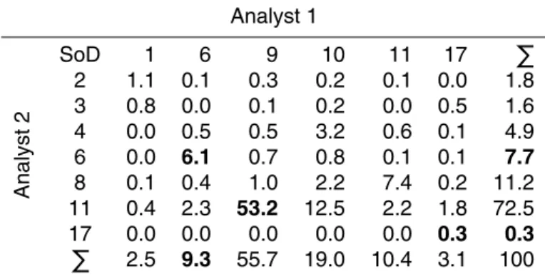
charts and the automatic segmentation. All pixels in the “Ice of Undefined SoD” class were excluded. The comparison was carried out by using a confusion matrix for each image pair (Table 1a–c). Each column in the confusion matrix represents one class in one chart, and each row represents one class in the other chart. All numbers in the confusion matrices are percentages of the total number of pixels in the chart, i.e. they 10

sum up to 100. By examining the entries in each confusion matrix we were able to state how each class in one chart relates to any of the classes in another chart.

4 Analysis

The analysis was carried out in two main steps. The first step included an intercom-parison of the manual ice charts and the automatic segmentation. The second step 15

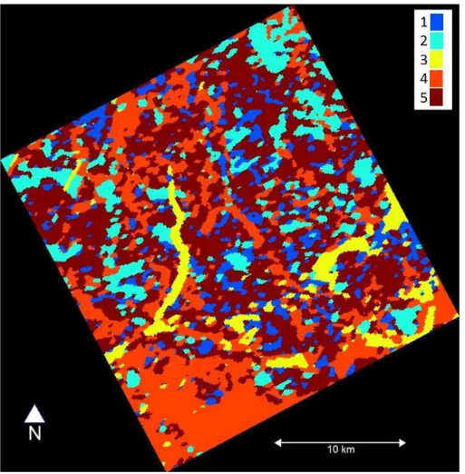
was to validate and interpret the automatically segmented image by using available in-situ data. The chart comparison was based on the smoothed, geocoded segmentation (Fig. 2b) and the two sea ice maps prepared by analyst 1 and analyst 2 (Fig. 4). In the manual ice charts each ice class/ice SoD is assigned a colour and a number. The legend is shown at the top of Fig. 4.

20

4.1 Comparison of the two hand-drawn ice charts

(14)

TCD

7, 2595–2634, 2013

Title Page

Tables Figures

◭ ◮

Back Close

Full Screen / Esc

Discussion

P

a

per

|

Di

scussion

P

a

per

|

Discussion

P

a

per

|

Discussi

on

P

a

per

|

However, a more detailed analysis showed some similarities in the segmentation, e.g., the purple segment at the bottom corner and the vertical lead in the middle of the im-age. By taking the labels into consideration, we noticed that the yellow (class 7) and all the green labels (classes 8–11) describe various stages of first-year ice. From a SAR imaging point-of-view, it is not possible to separate all these classes by visual inspec-5

tion of RGB images from polarimetric channel combinations. Merging all the first-year ice classes would make the ice charts more alike.

The confusion matrix from the comparison of the two hand-drawn ice charts is pro-vided in Table 1a. All numbers are given as percentages of the total number of pixels in the image. Important numbers to be discussed in the following are written in boldface. 10

The analysts label 9.3 % and 7.7 % of the pixels as Grey-White (class 6). This labeling is consistent for 6.1 % of the pixels, which is approximately a one-to-one correspon-dance. We would also like to highlight that the biggest classes, First stage First Year (class 9) in analyst 1’s chart and Medium First Year (class 11) in analyst 2’s ice chart, correspond very well. They are consistent for 53.2 % of the pixels. It is also worth noting 15

that all (100 %=0.3 %0.3 %) pixels in analyst 2’s class 17 (Nilas with frost flowers) is

classi-fied under analyst 1’s class 17. However, the opposite is not true, analyst 1’s class 17 is spread over several of analyst 2’s classes.

4.2 Comparison of hand-drawn ice charts and the automatic segmentation

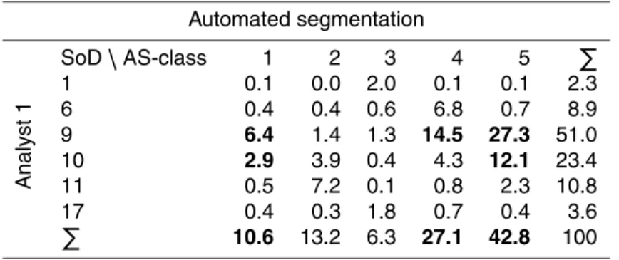
The intention of this section is to make a quantitative analysis of the relationships be-20

tween the ice maps. The confusion matrix from the comparison between analyst 1’s ice chart and the automatic segmentation is shown in Table 1b. Again, note that all percent-ages are relative to the total number of pixels in the image and important numbers to be discussed are written in boldface. A majority of the pixels in class 1 (60.4 %=10.6 %6.4 %),

class 4 (53.5 %=14.5 %27.1 %) and class 5 (63.8 %= 27.3 %

42.8 %) of the automatic segmentation 25

(15)

TCD

7, 2595–2634, 2013

Title Page

Tables Figures

◭ ◮

Back Close

Full Screen / Esc

Discussion

P

a

per

|

Di

scussion

P

a

per

|

Discussion

P

a

per

|

Discussi

on

P

a

per

|

many-to-one mapping also applies in the other direction, e.g. 87.7 % (=6.4 %_{10.6 %}+2.9 %) of class 1 in the automatic segmentation and 97.3 % (=27.3 %42.8 %+12.1 %) of class 5 in the

au-tomatic segmentation is distributed between analyst 1’s class 9 and 10. This indicates an inconsistency between the manual classification and the automated segmentation.

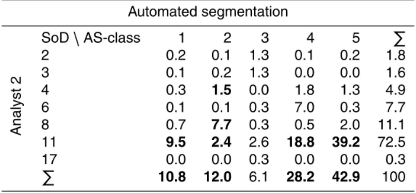
Table 1c shows the confusion matrix made from the comparison of analyst 2’s ice 5

chart and the automatic segmentation. Important numbers to be discussed are written in boldface. This comparison also shows a many-to-one mapping similar to the previous comparison. Now it is class 1 (88.0 %=10.8 %9.5 %), class 4 (67.0 %=

18.8 %

28.2 %) and class 5

(91.4 %=39.2 %42.9 %) in the automatic segmentation that are mapped into the dominating

Medium First Year class (class 11). As previously discussed, this class is known to 10

correspond to the First stage First Year class of analyst 1. The Young Ice (class 4) is also an example of a many-to-one mapping. This class is scattered into class 2,4 and 5 of the automatic segmentation. However, the many-to-one mapping applies in both directions. For example 97 % (=1.5 %+_{12.0 %}7.7 %+2.4 %) of class 2, in the automatic segmentation, is distributed between the young, the thin first-year and the medium 15

first-year ice. Once again we conclude that the manual classification and the automatic segmentation are inconsistent.

4.3 Validation and interpretation of the automatic segmentation

From the visual inspections and confusion matrices we established that the manual classifications and the automatic segmentation are inconsistent. The question that 20

arises is: which one of the maps is closest to the true physical ice types? The manually segmented ice charts are indisputably very subjective. They rely on the ice analyst’s experience, but also on the available amount of data, including satellite scenes and in-situ measurements.

On the other hand, the segments of the automatic segmentation must be labeled. An 25

(16)

TCD

7, 2595–2634, 2013

Title Page

Tables Figures

◭ ◮

Back Close

Full Screen / Esc

Discussion

P

a

per

|

Di

scussion

P

a

per

|

Discussion

P

a

per

|

Discussi

on

P

a

per

|

segments from the automatic segmentation (Fig. 5a), the Pauli image (Fig. 2a) and the unlabeled ice chart (Fig. 2b). The class descriptions they delivered are shown in Table 2. The yellow segments are various types of thin ice and open water, the red segments are young ice, occasionally deformed and/or with snow cover. Examples of optical photos taken from the helicopter from the open water/thin ice (yellow) class are 5

provided in Fig. 6. By examining the optical photos alone, the sea ice experts were not able to distinguish the blue, brown and the light blue segments. These were all first year ice, but could probably be characterized by their different degree of deforma-tion. However, by including the Pauli image, they were able to separate the light blue segments from the other classes. The light blue class appears dark in the Pauli image, 10

and is therefore interpreted as smoother than the brown and blue class. This is to some degree supported by a visual inspection of Fig. 5a.

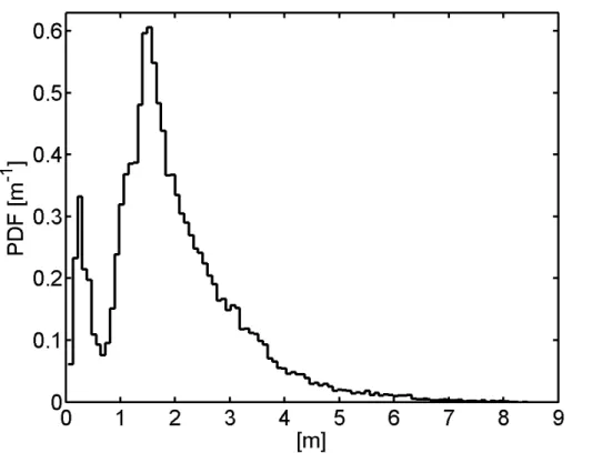
Ice thickness histograms for each class based on the EM-bird thickness measure-ments were utilized to examine the thickness-based class discrimination (Fig. 5b). The dominant ice thickness of each segment is denoted by the main peak whithin each 15

segment. However, the thickness histograms indicate mixed classes. This can occur as a result of coarse class boundaries and a co-location error of the EM-bird measure-ments and the satellite image. The latter is due to uncertainties in the drift correction. We trimmed each class region to avoid potentially contaminated thickness measure-ments close to the class boundaries.

20

The yellow class is very distinct from the other classes because of the large amount of open water/very thin ice and no ice thicker than 5 m (Fig. 5b). Before the trimming, the blue, light blue and brown classes are similar, which can explain the ice expert’s difficulties to separate them. In the blue class, the fraction of ice thicker than 4 m is lower than for the other two. The blue and the brown have very similar shape in the 25

(17)

TCD

7, 2595–2634, 2013

Title Page

Tables Figures

◭ ◮

Back Close

Full Screen / Esc

Discussion

P

a

per

|

Di

scussion

P

a

per

|

Discussion

P

a

per

|

Discussi

on

P

a

per

|

To further investigate the class discrimination we exploited physical information in the polarimetric features used in the segmentation algorithm. Our main attention was to examine the possibility to discriminate the three classes (blue, brown and light blue) that the ice experts were unable to separate. We expected the automatic segmentation to be influenced by outliers. For each of the six features we chose to calculate the me-5

dian and the median absolute deviation about the median (MADAM). These two robust statistics are not unduly affected by outliers. Given the data setX=X₁,X₂,. . .,X_N, the MADAMvalue is given by:

MADAM=median(_|Xi−median(X)|). (9)

The results are shown in Fig. 7. The probability density functions (pdf’s) for each class 10

and each feature are shown in Fig. 8. All six features, and especially the co-pol ratio (Fig. 7d), separate the open water/thin ice (yellow) class very well. The co-pol ratio is sensitive to the dielectric constants of the water and ice, thus it is expected to dis-criminate the water and ice. The brightness feature is responsive to roughness. The blue class is the brightest, and thus we interpret it to be the most deformed ice type, 15

the light blue class is the darkest one, and thus interpreted as smooth ice. This is in agreement with the light blue class being dark in the Pauli image. The cross-pol ratio is known to increase with deformation. Of the three classes we consider, Figs. 7c and 8c imply that the blue class is the most deformed and the light blue is the least deformed. This is consistent with the findings from the brightness feature and visual inspection 20

of the Pauli image. The results from the inverseRK feature is shown in Fig. 7a. This feature is expected to be sensitive to deformation and inhomogeneous surfaces. The blue, brown and light blue classes appear to be well separated. Of these three, the blue class has the lowest values, indicating that it contains the most deformed ice. The light blue has the highest values and is interpreted as smooth ice. All this is in accordance 25

(18)

TCD

7, 2595–2634, 2013

Title Page

Tables Figures

◭ ◮

Back Close

Full Screen / Esc

Discussion

P

a

per

|

Di

scussion

P

a

per

|

Discussion

P

a

per

|

Discussi

on

P

a

per

|

5 Discussion

Comparison of ice charts

The charts were not expected to be identical on a pixel level, due to the human factor in manual segmentation. Our investigation has shown though that all the charts are 5

inconsistent. This inconsistency may occur for several reasons:

– The number of classes disagree in all ice charts. We believe that the ice analysts have used too many classes in their interpretation, i.e., it is not possible to distin-guish five different stages of first year ice by visual inspection of a SAR image. The manual charts would probably be more similar if the number of classes and 10

their labels were set in advance.

– The hand-drawn polygons have rough boundaries and poor detail, which could

be a reason for the many-to-one mapping. More essentially, we believe the au-tomated algorithm interprets the image information more rigorously, thus distin-guishing more segments.

15

– The segmentation may fail over some complex parts of the scene where the ice

is heterogeneous and the detail level is high.

– The education and experience of the ice analysts may be one reason why the

manually drawn charts di_ffer. The analysts have little or no experience in thickness classification based on quad-pol images.

20

Class labeling

(19)

TCD

7, 2595–2634, 2013

Title Page

Tables Figures

◭ ◮

Back Close

Full Screen / Esc

Discussion

P

a

per

|

Di

scussion

P

a

per

|

Discussion

P

a

per

|

Discussi

on

P

a

per

|

or at ice/water boundaries are not representative for one specific class. Secondly, the EM-bird is not solely measuring the ice thickness. The measurements comprise the total snow and ice thickness. Optical images aid the interpretation of the segments, but the snow cover hampers the class labeling. Thus, distinguishing ice types based on thickness measurements (Fig. 5b) is not a trivial task. We see that the trimmed dataset 5

has lighter tails than the original dataset, for some of the classes. The effect is most visible for the smooth ice (class 2) and the open water/thin ice (class 3). This indicates that the results are affected by (1) imperfect co-location of the EM-bird measurements and the polSAR measurements, (2) blurring effects within the EM-bird footprint.

Polarimetric parameters

10

In order to compare our polarimetric parameters to values reported by others, we cal-culated the mean value and standard deviation (Table 3). In the subsequent discussion the co-pol ratio is given in dB. We found the mean co-pol ratio,R_VV_/_HH, to be largest and have the largest variability for open water/thin ice (class 2), which is in agreement 15

with the findings of Geldsetzer and Yackel (2009). The other classes were close to zero, except for class 2. By re-defining the co-pol ratio as RHH/VV, we found it to be

positive for all ice types except for open water/thin ice, which is in accordance with the findings of Gill and Yackel (2012) and Drinkwater et al. (1992). Scheuchl et al. (2001) also reported negative co-pol values for open water. Gill and Yackel (2012) reported 20

the co-pol ratio to increase with incidence angle for all positive values and decrease for open water. The incidence angle of our scene is less than the one in Drinkwater et al. (1992) and exceeds those used in Gill and Yackel (2012). We see that our co-pol ratio for open water/thin ice follows the trend and extrapolate those values found by Gill and Yackel (2012) and Drinkwater et al. (1992).

25

(20)

TCD

7, 2595–2634, 2013

Title Page

Tables Figures

◭ ◮

Back Close

Full Screen / Esc

Discussion

P

a

per

|

Di

scussion

P

a

per

|

Discussion

P

a

per

|

Discussi

on

P

a

per

|

(Drinkwater et al., 1992), which supports that all our co-pol correlation magnitudes are less than those reported by Gill and Yackel (2012). However, they reported the co-pol correlation magnitude of open water to be the greatest. We found two classes, open water/thin ice and class 4, to have equally large co-pol correlation magnitude.

We found the mean co-pol correlation angle to be positive for all ice types. This does 5

not coincide with the work of Gill and Yackel (2012), which reports negative angles for all ice types and open water. However, our findings correspond well with what was reported by Dierking et al. (2003), with one exception. They found that open water had

negative phase differences. We found that the most deformed ice (class 1) had the

larges value. The young ice type had the smallest mean angle. Gill and Yackel (2012) 10

reported negative mean phase di_fferences at all incidence angles and for all ice types.

6 Conclusions

We have shown that the manual and the automatic generated segmentation maps dis-agree. Even the two manual charts are inconsistent to some degree. Manually drawn ice charts are commonly used for validation of automatic classification algorithms (Za-15

khvatkina et al., 2013; Kwon et al., 2013). This study has shown that the SoD charts should be used with care for validation purposes.

Our results suggests that utilizing polarimetric parameters in sea ice classification improves the classification accuracy. TheRK parameter, which has not previously been used for ice segmentation, distinguishes well between deformed and smooth ice and 20

makes a valuable contribution to the segmentation.

The automatic algorithm separates the satellite scene into a given number of classes. The six features used as input to the algorithm should also be able to distinguish multi year ice, but our scene did not contain any multi year ice.

The automatic algorithm separated the SAR scene into five unlabeled classes. The 25

(21)

TCD

7, 2595–2634, 2013

Title Page

Tables Figures

◭ ◮

Back Close

Full Screen / Esc

Discussion

P

a

per

|

Di

scussion

P

a

per

|

Discussion

P

a

per

|

Discussi

on

P

a

per

|

remaining unlabeled classes in terms of deformation level. The physical interpretation of the co-pol correlation angle and magnitude for medium and thick ice should be fur-ther investigated if they shall be used in class labeling.

The number of classes is a critical input parameter which constrains the algorithm. If the number is too low, some segments will contain class mixtures. If the number is too 5

high, the algorithm splits real ice classes, simply to attain the given number of classes. We found in our validation testing (Sect. 4.3) that the yellow class clearly is bimodal and should be split (see Fig. 8). This is in line with the interpretation of the ice experts (Table 2). This indicates that the constrained number of classes for the segmentation algorithm should be increased.

10

If the number of classes is increased by one, the algorithm will partition the data based on statistical criteria of optimality. This will not necessarily enforce the desired result, which is to split the bimodal class. Class boundaries may change and other classes may split, which is what we have experienced in our search for the seemingly optimal number of classes.

15

Future work should focus on automatic and robust estimation of the number of classes, while noting that this is an inherently complicated problem, especially for highly detailed and heterogeneous sea ice scenes. For operational ice charting, automatic la-beling will increase the efficiency compared to today’s manual interpretation of SAR images. The labeling can be based on polarimetric parameters with a clear physical 20

interpretation and statistical distribution models for these parameters.

Polarimetric SAR images makes it possible to segment and label ice classes based on physical properties. The polarimetric SAR data format is currently not suitable for operational ice charting, due to its limited swath width. However, the emerging compact polarimetry mode implemented on future sensors like PALSAR-2 and the Radarsat 25

(22)

TCD

7, 2595–2634, 2013

Title Page

Tables Figures

◭ ◮

Back Close

Full Screen / Esc

Discussion

P

a

per

|

Di

scussion

P

a

per

|

Discussion

P

a

per

|

Discussi

on

P

a

per

|

Acknowledgements. The authors acknowledge Vera Lund and Trond Robertsen of the

Norwe-gian Ice Service for their analysis of sea ice stage of development and Thomas Kræmer at the University of Tromsø for advice in the geocoding process. We are grateful to the captain and crew onboard the Norwegian coast guard vessel Svalbard and the Airlift pilots and technicians onboard AS 350 and Dauphin for their assistance during the research cruise. This project was 5

supported financially by the project “Sea Ice in the Arctic Ocean, Technology and Systems of Agreements” (“Polhavet”, subproject “CASPER”) of the Fram Centre, and by the Centre for Ice, Climate and Ecosystems at the Norwegian Polar Institute. We are also funded by RDA Troms.

References

Bogdanov, A. V., Sandven, S., Johannessen, O. M., Alexandrov, V. Y., and Bobylev, L. P.: Multi-10

sensor approach to automated classification of sea ice image data, IEEE T. Geosci. Remote, 43, 1648–1663, 2005. 2598

Breivik, L.-A., Eastwood, S., Karvonen, J., Dinessen, F., Fleming, A., Hamre, T., Pedersen, L. T., Saldo, R., and Buus-Hinkler, J.: Quality information document for OSI TAC sea ice products 011-001, -002, -003, -004, -006, -007, -009, -010, -011, -012, Technical report MYO2-OSI-15

QUID-011-ALL, version 1.3, available at: http://catalogue.myocean.eu.org/static/resources/ myocean/quid/MYO2-OSI-QUID-011-ALL-V1.3.pdf, Oslo, 2012. 2598

Charbonneau, F., Brisco, B., Raney, R. K., McNairn, H., Liu, C., Vachon, P., Shang, J., DeAbreu, R., Champagne, C., Merzouki, A., and Geldsetzer, T.: Compact polarimetry over-iew and applications assessment, Can. J. Remote Sens. (Suppl.), 36, S298–S315, 2010. 20

2615

Clausi, D. A. and Deng, H.: Operational Segmentation and Classification of SAR Sea Ice Im-agery, IEEE Workshop on Advances in Techniques for Analysis of Remotely Sensed Data, 268–275, 2004. 2597, 2598

Clausi, D. A., Qin, A. K., Chowdhury, M. S., Yu, P., and Maillard, P.: MAGIC: MAp-Guided Ice 25

Classification system, Can. J. Remote Sens. (Suppl.), 36, S13–S25, 2010. 2598

(23)

TCD

7, 2595–2634, 2013

Title Page

Tables Figures

◭ ◮

Back Close

Full Screen / Esc

Discussion

P

a

per

|

Di

scussion

P

a

per

|

Discussion

P

a

per

|

Discussi

on

P

a

per

|

Dierking, W., Skriver, H., and Gudmandsen, P.: SAR Polarimetry for Sea Ice Classification, in: Proc. PolinSAR 2003, 109–118, 2003. 2598, 2614

Doulgeris, A. and Eltoft, T.: Scale Mixture of Gaussian modelling of polarimetric SAR data, EURASIP J. Adv. Sig. Pr., 2010, 1–12, doi:10.1155/2010/874592, 2010. 2604, 2606

Drinkwater, M. R., Kwok, R., Rignot, E., Israelsson, H., Onstott, R. G., and Winebrenner, D. P.: 5

Potential applications of polarimetry to the classification of sea ice, in: Microwave Remote Sensing of Sea Ice, no. 68 in Geophysical Monograph, edited by: Carsey, F. D., AGU, 419– 430, 1992. 2605, 2613, 2614

Geldsetzer, T. and Yackel, J. J.: Sea ice type and open water discrimination using dual co-polarized C-band SAR, Can. J. Remote Sens., 35, 73–84, 2009. 2598, 2613

10

Gill, J. and Yackel, J.: Evaluation of C-band SAR polarimetric parameters for discriminating of first-year sea ice types, Can. J. Remote Sens., 38, 306–323, 2012. 2598, 2605, 2613, 2614 Haas, C., Lobach, J., Hendricks, S., Rabenstein, L., and Pfa_ffling, A.: Helicopterborne mea-surements of sea ice thickness, using a small and lightweight, digital em system, J. Appl. Geophys., 67, 234–241, 2009. 2601

15

Hara, Y., Atkins, R. G., Shin, R. T., Kong, J. A., Yueh, S. H., and Kwok, R.: Application of neural networks for sea ice classification in polarimetric SAR images, IEEE T. Geosci. Remote, 33, 740–748, 1995. 2598

Hartigan, J. A.: Clustering Algorithms, Wiley, New York, 1975. 2598

Karvonen, J.: C-band sea ice SAR classification based on segmentwise edge features, in: Geo-20

science and Remote Sensing New Achievements, edited by: Imperatore, P. and Riccio, D., In-Tech, available at: http://www.intechopen.com/books/geoscience-and-remotesensing-new-achievements/c-band-sea-ice-sar-classification-based-on-segmentwise-edge-features, 2010. 2598

Karvonen, J. A.: Baltic sea ice SAR segmentation and classification using modified pulse-25

coupled neural networks, IEEE T. Geosci. Remote, 42, 1566–1574, 2004. 2598, 2606 Kwok, R., Rignot, E., and Holt, B.: Identification of sea ice types in spaceborne Synthetic

Aper-ture Radar data, J. Geophys. Res, 97, 2391–2402, 1992. 2606

Kwok, R., Cunningham, G. F., Wensnahan, M., Rigor, I., Zwally, H. J., and Yi, D.: Thinning and volume loss of the Arctic Ocean sea ice cover: 2003–2008, J. Geophys. Res, 114, C07005, 30

(24)

TCD

7, 2595–2634, 2013

Title Page

Tables Figures

◭ ◮

Back Close

Full Screen / Esc

Discussion

P

a

per

|

Di

scussion

P

a

per

|

Discussion

P

a

per

|

Discussi

on

P

a

per

|

Kwon, T.-J., Li, J., and Wong, A.: ETVOS: an enhanced total variation optimization segmenta-tion approach for SAR sea-ice image segmentasegmenta-tion, IEEE T. Geosci. Remote, 51, 925–934, 2013. 2598, 2614

Lee, J.-S. and Pottier, E.: Polarimetric Radar Imaging, from Basics to Applications, Taylor & Francis Group, 2009. 2599, 2600

5

MANICE: Manual of Standard Procedures for Observing and Reporting Ice Conditions, Canadian Ice Service, ISBN: 0-660-62858-9, available at: http://www.ec.gc.ca/glaces-ice/ 4FF82CBD-6D9E-45CB-8A55-C951F0563C35/MANICE.pdf, 2005. 2602

Maslanik, J., Stroeve, J., Fowler, C., and Emery, W.: Distribution and trends in Arctic sea ice age through spring 2011, Geophys. Res. Lett., 38, L13502, doi:10.1029/2011GL047735, 2011. 10

2596

Mundy, C. J. and Barber, D. A.: On the relationship between spatial patterns of sea-ice type and the mechanisms which create and maintain the North Water (NOW) polynya, Atmos. Ocean, 39, 327–341, 2001. 2606

Ochilov, S. and Clausi, D.: Automated classification of operational SAR sea ice images, Proc. 15

Canadian Conference Computer and Robot Vision, 40–45, 2010. 2598

Onstott, R. G. and Shuchman, R. A.: Synthetic aperture radar marine user’s manual, in: SAR Measurements of Sea Ice, edited by: Jackson, C. and Apel, J. R., NOAA, 81–115, 2004. 2605, 2606

Renner, A. H. H., Hendricks, S., Gerland, S., Beckers, J., Haas, C., and Krumpen, T.: Large-20

scale ice thickness distribution of first-year sea ice in spring and summer north of Svalbard, Ann. Glaciol., 54, 13–18, 2013. 2601

Samadani, R.: A finite mixtures algorithm for finding proportions in SAR images, IEEE T. Image Process., 4, 1182–1186, 1995. 2598

Scheuchl, B., Caves, R., Cumming, I., and Staples, G.: Automated Sea Ice Classification Using 25

Spaceborne Polarimetric SAR Data, in: Proc. IGARSS 2001, 3117–3119, 2001. 2598, 2605, 2613

Scheuchl, B., Hajnsek, I., and Cumming, I.: Sea ice classification using multi-frequency polari-metric SAR data, IGARSS, 3, 1914–1916, 2002. 2598

Scheuchl, B., Hajnsek, I., and Cumming, I.: Classification strategies for polarimetric SAR sea 30

ice data, in: Proc. PolinSAR 2003, 57.1–57.6, 2003. 2598

(25)

TCD

7, 2595–2634, 2013

Title Page

Tables Figures

◭ ◮

Back Close

Full Screen / Esc

Discussion

P

a

per

|

Di

scussion

P

a

per

|

Discussion

P

a

per

|

Discussi

on

P

a

per

|

Thomsen, B., Pedersen, L., Skriver, H., and Dierking, W.: Polarimetric EMISAR observations of sea ice in the Greenland Sea, in: Future Trends in Remote Sensing, edited by: Gudmand-sen, P., Taylor & Francis, 345–351, 1998b. 2606

Yu, Q. and Clausi, D. A.: IRGS: image segmentation using edge penalties and region growing, IEEE T. Pattern Anal., 30, 2126–2139, 2008. 2598

5

(26)

TCD

7, 2595–2634, 2013

Title Page

Tables Figures

◭ ◮

Back Close

Full Screen / Esc

Discussion

P

a

per

|

Di

scussion

P

a

per

|

Discussion

P

a

per

|

Discussi

on

P

a

per

|

Table 1a.Confusion matrix for hand-drawn ice charts (Fig. 4). SoD is the ice stage of develop-ment defined by WMO. Numbers are given in %.

Analyst 1

Analyst

2

SoD 1 6 9 10 11 17 P

2 1.1 0.1 0.3 0.2 0.1 0.0 1.8

3 0.8 0.0 0.1 0.2 0.0 0.5 1.6

4 0.0 0.5 0.5 3.2 0.6 0.1 4.9

6 0.0 6.1 0.7 0.8 0.1 0.1 7.7

8 0.1 0.4 1.0 2.2 7.4 0.2 11.2

11 0.4 2.3 53.2 12.5 2.2 1.8 72.5

17 0.0 0.0 0.0 0.0 0.0 0.3 0.3

P

(27)

TCD

7, 2595–2634, 2013

Title Page

Tables Figures

◭ ◮

Back Close

Full Screen / Esc

Discussion

P

a

per

|

Di

scussion

P

a

per

|

Discussion

P

a

per

|

Discussi

on

P

a

per

|

Table 1b.Confusion matrix for automated segmentation (Fig. 2b) and analyst 1’s ice chart (Fig. 4). SoD is the ice stage of development defined by WMO. AS-class is the unlabeled segments from the automated segmentation. Numbers are given in %.

Automated segmentation

Analyst

1

SoD_\AS-class 1 2 3 4 5 P

1 0.1 0.0 2.0 0.1 0.1 2.3

6 0.4 0.4 0.6 6.8 0.7 8.9

9 6.4 1.4 1.3 14.5 27.3 51.0

10 2.9 3.9 0.4 4.3 12.1 23.4

11 0.5 7.2 0.1 0.8 2.3 10.8

17 0.4 0.3 1.8 0.7 0.4 3.6

P

(28)

TCD

7, 2595–2634, 2013

Title Page

Tables Figures

◭ ◮

Back Close

Full Screen / Esc

Discussion

P

a

per

|

Di

scussion

P

a

per

|

Discussion

P

a

per

|

Discussi

on

P

a

per

|

Table 1c.Confusion matrix for automated segmentation and analyst 2’s ice chart. SoD is the ice stage of development defined by WMO. AS-class is the unlabeled segments from the auto-mated segmentation. Numbers are given in %.

Automated segmentation

Analyst

2

SoD_\AS-class 1 2 3 4 5 P

2 0.2 0.1 1.3 0.1 0.2 1.8

3 0.1 0.2 1.3 0.0 0.0 1.6

4 0.3 1.5 0.0 1.8 1.3 4.9

6 0.1 0.1 0.3 7.0 0.3 7.7

8 0.7 7.7 0.3 0.5 2.0 11.1

11 9.5 2.4 2.6 18.8 39.2 72.5

17 0.0 0.0 0.3 0.0 0.0 0.3

P

(29)

TCD

7, 2595–2634, 2013

Title Page

Tables Figures

◭ ◮

Back Close

Full Screen / Esc

Discussion

P

a

per

|

Di

scussion

P

a

per

|

Discussion

P

a

per

|

Discussi

on

P

a

per

|

Table 2. Class labels produced by sea ice experts. The colours refer to those in automatic segmentation (Fig. 2b) and are the same in Figs. 5–8.

Segment colour (class number) Stage of Development (SoD)

Blue(1)/Light Blue(2)/Brown(5) First year ice,

different stages of development

Yellow(3) Thin ice,

open water, new ice, nilas, grey ice

Red(4) Young ice, thin first year ice

(30)

TCD

7, 2595–2634, 2013

Title Page

Tables Figures

◭ ◮

Back Close

Full Screen / Esc

Discussion

P

a

per

|

Di

scussion

P

a

per

|

Discussion

P

a

per

|

Discussi

on

P

a

per

|

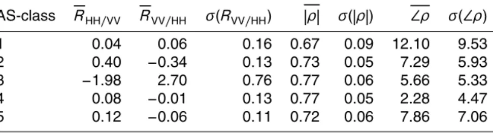
Table 3.Mean and standard deviation for the polarimetric features: co-pol ratio (R_HH_/_VV and

R_VV_/_HH) given in dB, co-pol correlation magnitude (_|ρ_|) and co-pol correlation angle (∠_ρ_{) given in}

degrees. The operators () andσ() represents the mean and the standard deviation, respectively. AS-class is the unlabeled segments from the automated segmentation.

AS-class R_HH_/_VV R_VV_/_HH σ(R_VV_/_HH) _|ρ_| σ(_|ρ_|) ∠_ρ _σ₍∠_ρ₎

1 0.04 0.06 0.16 0.67 0.09 12.10 9.53

2 0.40 −0.34 0.13 0.73 0.05 7.29 5.93

3 −1.98 2.70 0.76 0.77 0.06 5.66 5.33

4 0.08 ₋0.01 0.13 0.77 0.05 2.28 4.47

(31)

TCD

7, 2595–2634, 2013

Title Page

Tables Figures

◭ ◮

Back Close

Full Screen / Esc

Discussion

P

a

per

|

Di

scussion

P

a

per

|

Discussion

P

a

per

|

Discussi

on

P

a

per

|

(32)

TCD

7, 2595–2634, 2013

Title Page

Tables Figures

◭ ◮

Back Close

Full Screen / Esc

Discussion

P

a

per

|

Di

scussion

P

a

per

|

Discussion

P

a

per

|

Discussi

on

P

a

per

|

(33)

TCD

7, 2595–2634, 2013

Title Page

Tables Figures

◭ ◮

Back Close

Full Screen / Esc

Discussion

P

a

per

|

Di

scussion

P

a

per

|

Discussion

P

a

per

|

Discussi

on

P

a

per

|

(34)

TCD

7, 2595–2634, 2013

Title Page

Tables Figures

◭ ◮

Back Close

Full Screen / Esc

Discussion

P

a

per

|

Di

scussion

P

a

per

|

Discussion

P

a

per

|

Discussi

on

P

a

per

|

(35)

TCD

7, 2595–2634, 2013

Title Page

Tables Figures

◭ ◮

Back Close

Full Screen / Esc

Discussion

P

a

per

|

Di

scussion

P

a

per

|

Discussion

P

a

per

|

Discussi

on

P

a

per

|

(36)

TCD

7, 2595–2634, 2013

Title Page

Tables Figures

◭ ◮

Back Close

Full Screen / Esc

Discussion

P

a

per

|

Di

scussion

P

a

per

|

Discussion

P

a

per

|

Discussi

on

P

a

per

|

(37)

TCD

7, 2595–2634, 2013

Title Page

Tables Figures

◭ ◮

Back Close

Full Screen / Esc

Discussion

P

a

per

|

Di

scussion

P

a

per

|

Discussion

P

a

per

|

Discussi

on

P

a

per

|