Mapsnp: An R Package to Plot a Genomic
Map for Single Nucleotide Polymorphisms
Fuquan Zhang1,2☯, Yong Xu3☯, Hongbao Cao2, Chunhui Jin1, Zaohuo Cheng1,
Guoqiang Wang1*, Yin Yao Shugart2*
1Wuxi Mental Health Center of Nanjing Medical University, Wuxi, Jiangsu Province, China,2Unit on Statistical Genomics, Intramural Research Program, National Institute of Mental Health, National Institutes of Health, Bethesda, Maryland, United States of America,3Department of Psychiatry, First Hospital of Shanxi Medical University, Taiyuan, China
☯These authors contributed equally to this work.
*[email protected](GW);[email protected](YYS)
Abstract
Single-nucleotide polymorphism (SNP) is one of the most common sources of genetic varia-tions of the genome. Currently, SNPs are a main target for most genetic association studies. Visualizing genomic coordinates of SNPs, including their physical location relative to their host gene, and the structure of the relevant transcripts, may provide intuitive supplements to the understanding of their functions. Nevertheless, to date, no such easy-to-use program-ming tools exist. Therefore, we developed an R package,“mapsnp”, to plot genomic map for a panel of SNPs within a genome region of interest, including the relative chromosome location and the transcripts in the region. mapsnp is a simple and flexible software package which can be used to visualize a genomic map for SNPs, integrating a chromosome ideo-gram, genomic coordinates, SNP locations and SNP labels.
Introduction
Single-nucleotide polymorphism (SNP) is one of the most common sources of genetic varia-tions of the genome. Currently, many genetic studies, including genome-wide association study (GWAS) use SNPs as their research tools. Visualizing SNP data in a graph may provide a clear and intuitive impression for the reader. Various visualization tools have been developed, most of which have been implemented in the form of a genome browser. The NCBI genome browsers [1] distributes genome annotations and provides integrated views of valuable geno-mic data for supported genomes. The UCSC [2] and Ensembl Genome Browser [3] offer online tools for visualizing a set of annotation‘tracks’for a genomic region. These web applications provide analysis and retrieval resources and serve as reference datasets for individual SNPs or genes. Nevertheless, these tools have limited plotting options and are not programmatically ac-cessible. For example, these tools cannot be used to yield annotation tracks for a specific set of SNPs within a genomic region of interest, due to their lack of flexibility.
The statistical programming environment R [4] provides a plethora of methods and tools to analyze and visualize data. There are several programming tools for visualizing genomic data,
OPEN ACCESS
Citation:Zhang F, Xu Y, Cao H, Jin C, Cheng Z, Wang G, et al. (2015) Mapsnp: An R Package to Plot a Genomic Map for Single Nucleotide
Polymorphisms. PLoS ONE 10(4): e0123609. doi:10.1371/journal.pone.0123609
Academic Editor:Jonathan Arthur, Children's Medical Research Institute, AUSTRALIA
Received:July 14, 2014
Accepted:March 4, 2015
Published:April 8, 2015
Copyright:This is an open access article, free of all copyright, and may be freely reproduced, distributed, transmitted, modified, built upon, or otherwise used by anyone for any lawful purpose. The work is made
available under theCreative Commons CC0public
domain dedication.
Data Availability Statement:All relevant data are within the paper and its Supporting Information files.
such as GenomeGraphs [5], ggbio [6], and Gviz [7]. Within these packages, individual types of genomic features or data are represented by separate tracks, and there are constructor tions to coordinate and plot these tracks. Yet, none of these packages provide a specific func-tion to plot detailed informafunc-tion for a panel of user-specified SNPs.
We developed mapsnp, as an add-on software package for the statistical programming envi-ronment R, to facilitate the integrated visualization of genomic maps for SNPs of interest.
Methods and Implementations
Program description
Our function leverages the statistical functionality available in R, the grammar of graphics and the data handling capabilities of the Bioconductor project [8]. mapsnp employs the Gviz sys-tem [7] to plot a genomic map for candidate SNPs. Biological scientists often confront the need to plot genomic data, along with a variety of genomic annotation features, such as gene or tran-script models, CpG island, and genetic variations. These features may be extracted from public data bases like PubMed, Ensembl, or UCSC. The Gviz package provides a structured visualiza-tion framework to plot any type of data along genomic coordinates. All plots are done using the grid graphics system, and several specialized annotation classes allow the integration of publicly available genomic annotation data from sources like UCSC [2] or Ensembl [3]. The ra-tionale behind the Gviz package is that individual types of genomic features or data are repre-sented by separate tracks. Each track constitutes a single object inheriting from class GdObject, and there are constructor functions to plot these tracks. When combining multiple objects, the individual tracks will always share the same genomic coordinate system, thus automatically aligning the plot elements.
A SNP map plotted by mapsnp includes five tracks: a chromosome ideogram track, a geno-mic coordinate track, a transcript track, a SNP location track, and a SNP label track.
An ideogram is a simplified visual representation of a chromosome, with the different chro-mosomal staining bands indicated by color, and the centromere indicated by shape. The neces-sary information to produce this visualization is stored in online data repositories, for instance at UCSC (http://genome.ucsc.edu/). Unlike all other track objects, ideogram tracks are not dis-played on the same coordinate system. Instead, the current genomic location is indicated on the chromosome by a red box that sits on the ideogram image. This track shows the currently displayed region in the broader context of the whole chromosome, indicating how much of the complete chromosome is covered in our plot.
The genomic coordinate track is always relative to the other plotted tracks, thus there is little need for additional function arguments to adjust its output.
For the transcript track, the‘msa’function calls the biomaRt package [9] to perform on-line annotation queries to Ensembl [3] and then translates these to transcript structures. The‘msb’ function utilizes Homo Sapiens data from UCSC based on the knownGene table, implemented in the‘TxDb.Hsapiens.UCSC.hg19.knownGene’package [10].
The SNP location track indicates genomic base-pair location of SNPs, while the SNP label track annotates their ID number.
Since the mapsnp package inherits from the Gviz package, detailed rationales or algorithms for each of these tracks can be found at Gviz’s online user guide (http://www.bioconductor.org/ packages/release/bioc/html/Gviz.html).
Functionality
The mapsnp package contains two functions,‘msa’and‘msb’. Both functions have three neces-sary arguments,‘M’,‘start’, and‘end’. The major parameter‘M’is a three-column matrix or
data frame, including chromosome, SNP ID, and SNP’s genomic location. The‘start’and‘end’ indicate the range of a highlighting region, typically a gene region corresponding to the mapped SNPs. The package offers multiple options to fine-tune the track appearance. Display parameters control the look of a track by defining properties of individual track objects.
The genomic coordinate track determines plotted genomic range. There is no need to know in advance about a particular genomic location when constructing the map. Instead, the plotted genomic range will be determined automatically from the context. Our package will display the region from the leftmost item to the rightmost item in any of the tracks. We often wish to zoom in or out on a particular plotting region to see more details or to get a broader overview. To that end, the‘start’and‘end’arguments let us choose an arbitrary genomic range to plot. Another pair of arguments that control the zoom state are‘extendL’and‘extendR’. These argu-ments are relative to the currently displayed ranges, and can be used to extend the view on one or both ends of the plot. The argument‘axisLabPos’controls the arrangement of the tick marks. It takes one of the values‘alternating’,‘above’or‘below’.
For the transcript track, one can control the horizontal stacking of overlapping items using the‘stacking’display parameter. Presently, the three values squish (making best use of the avail-able space), dense (no stacking at all) and hide (not showing the track items at all) are supported.
The‘SNPidPos’parameter controls the vertical positioning of the SNP ID labels, with three values (‘alternating’,‘above’or‘below’). The‘alternating’will construct two SNP label tracks, with one above the SNP location track and the other below the SNP location track.
There are dozens of other parameters, which fine-tune other track properties, such as color, size, track name, annotation text, and so on. The detailed usage of the package is described in Supporting InformationS1 File.
Built-in SNP dataset
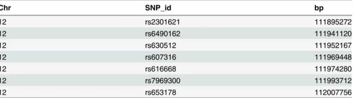
The built-in dataset involving seven candidate SNPs within the ATXN2 gene, from a genetic association study of schizophrenia [11]. As shown inTable 1, the dataset includes 7 SNPs with-in the ATXN2 gene, with-involvwith-ing three columns: the first column is chromosome, the second col-umn is SNP ID, and the third colcol-umn is SNP genomic location.
Results
Application on the SNP data
To illustrate the use of mapsnp, we show an example for‘msa’on the built-in dataset involving seven candidate SNPs within the ATXN2 gene. The genomic range of this gene is from 111950277 to 112036294 base-pair.
Table 1. Seven SNPs in ATXN2
Chr SNP_id bp
12 rs2301621 111895272
12 rs6490162 111941120
12 rs630512 111952167
12 rs607316 111969448
12 rs616668 111974280
12 rs7969300 111993712
12 rs653178 112007756
Chr: chromosome; bp: base pair
Load the mapsnp package and the snp data:
• library(mapsnp)
• data(snp)
• msa(M = snp, start = 111950277, end = 112036294, SNPidPos =‘alternating’)
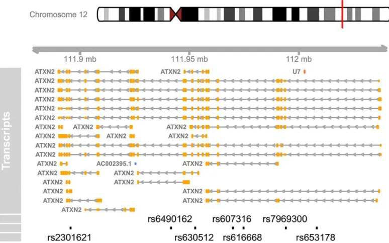
The above command plots a genomic map for the ATXN2 SNPs, with multiple alternative transcripts (Fig 1). Please note that users need an established internet connection for the pack-age to work, and that fetching data from UCSC can take some time. Usually, there might be dozens of transcripts for a gene, and the longer a gene is, the more transcripts it has. Therefore, the transcript track may seem redundant for large genes. In many situations, it may be more desirable to create a concise map with all the transcripts stacking together. Nevertheless, there is a caveat in doing so, as there are some transcripts for other overlapping genes within the ge-nomic region, for instance U7 and AC230095.1 inFig 1. When combining multiple transcripts together, the intended transcript ATXN2 will contain other‘noisy’transcripts as well.
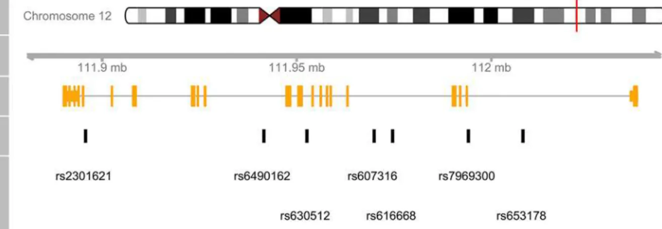
To circumvent the above issue, we created another function, msb, which leverages existent UCSC dataset curated by the‘TxDb.Hsapiens.UCSC.hg19.knownGene’package for the con-struction of a transcript track. It contains only the major transcripts within the genomic region. Thus, multiple transcripts can be safely merged together to produce a concise genomic map.
Fig 1. A detailed genomic map for seven SNPs within ATXN2 using Ensembl database.At the top, the relevant chromosome is drawn with the subregion of interest marked in red. The‘Transcript’track shows all the alternative transcripts within the region, retrieved from Ensembl database, including a non-ATXN2 transcript U7. At the bottom, the SNPs’location and ID are plotted along the same genomic coordinate.
The following commands will load the dataset and plot a genomic map for the ATXN2 SNPs, with only one merged transcript (Fig 2).
Comparison with existing tools
Various visualization tools have been developed, most of which are implemented in the form of a genome browser. There are desktop-based browsers like Integrated Genome Browser [12] and Integrative Genomics Viewer [13], as well as web-based genome browsers like Ensembl, UCSC Genome Browser, and GBrowse [14]. These browsers can display genomic annotations and other features for a region, each with specific advantages for different purposes. However, web-based genome browsers cannot integrate custom-supplied data into the genomic map. Desktop-based browsers can display custom data alongside gene annotations, but they have difficulty manipulating feature tracks from foundation datasets and lack programming flexibil-ity. Programming tools like GenomeGraphs [5], ggbio [6], and Gviz [7] have the flexibility to coordinate and plot public genomic features and custom data. However, none of these packages offer a specific function to show genomic information for a panel of candidate SNPs.
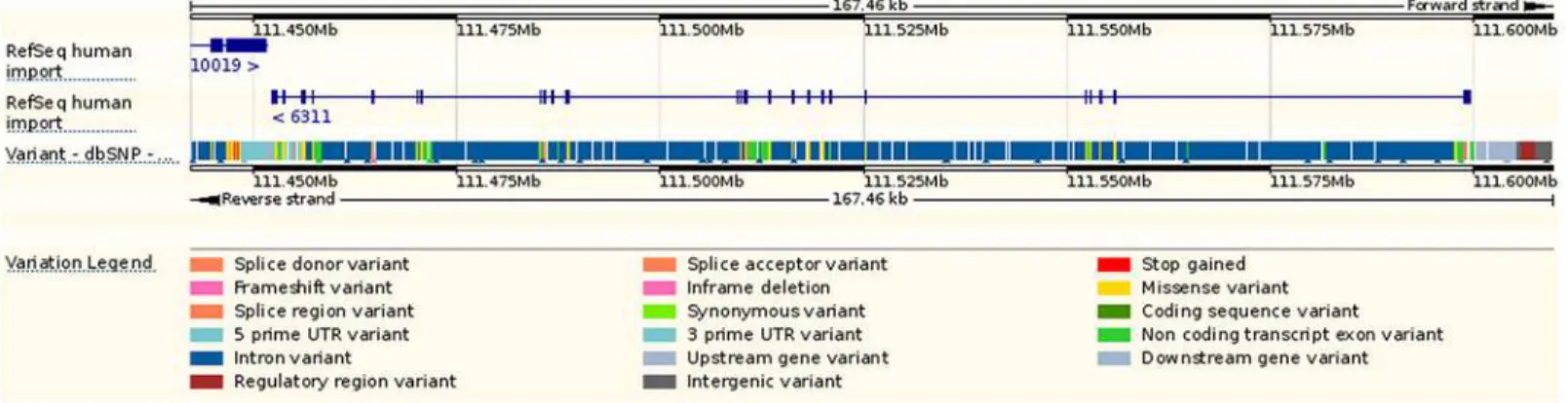
Since UCSC Genome Browser and Ensembl are two of the most commonly used genome vi-sualization tools, we utilized these two browsers to illustrate the genomic information of ATXN2 gene. With UCSC browser, we input the‘ATXN2’and selected a subset tracks to show its geno-mic features (Fig 3). Next, we made a gene-based display for ATXN2 in Ensembl (Fig 4). As shown inFig 3andFig 4, all of the common SNPs within ATXN2 were displayed. We could not select or highlight SNPs of interest within the gene.Fig 4also lacks an ideogram track.
To our knowledge, mapsnp is the only software package specifically designed to display ge-nomic information for SNPs of interest.
Fig 2. A concise genomic map for seven SNPs within ATXN2 using UCSC database.At the top, the relevant chromosome is drawn with the subregion of interest marked in red. The‘ATXN2’track shows the combined gene model of the alternative transcripts of the ATXN2 gene. At the bottom, the SNPs’
location and ID are plotted along the same genomic coordinate.>library(TxDb.Hsapiens.UCSC.hg19.knownGene)>msb(M = snp, start = 111950277,
end = 112036294, geneTrName =‘ATXN2’).
doi:10.1371/journal.pone.0123609.g002
Fig 3. A genomic map for ATXN2 via UCSC browser.
Discussion
Visualization is an important component of genomic analysis, because it facilitates exploration and discovery by revealing genomic patterns of variations [6]. Presently, most visualization tools are implemented in the form of a genome browser, which are unable to address user-supplied SNPs. mapsnp provides a new tool to visualize and explore genomics annotations for a group of SNPs. It mimics the layout of the popular UCSC Genome Browser, providing de-tailed views of SNP locations, genomic regions, summary views of splicing patterns, and ge-nome-wide overviews with a karyogram. Within the views, one can easily discern whether a SNP is located in exon, intron, 3’untranslated regions (UTR) or 5’UTR of a transcript, as well as get an overview of the distribution of a panel of SNPs relative to their host gene. The package is especially useful for most candidate gene studies by exploring genomic features for relevant SNPs.
The two functions implemented in the package are easy to use. We used this package to plot one gene in the example. However, the package can plot multiple adjacent genes simultaneous-ly. Meanwhile, the functions are flexible by offering dozens of parameters to fine-tune a final graph output, which are detailed in the package documentation. Future versions of the package will include more flexibility in terms of plotting parameters.
The major limitation of the mapsnp package may be its relatively slow executing speed, since the connection to the online data (UCSC) can take a certain amount of time (usually several minutes) depending on usage and network traffic. The other limitation lies in that only a single chromosome can be active during a given plotting operation. Consequently, we cannot plot multiple chromosomes in a single call to the function. However, we can build our own composite plots using multiple consecutive calls. It is best to plot no more than two or three dozen SNPs within a map, since too many SNPs will make it difficult to discriminate them.
In conclusion, we present mapsnp, a software tool designed to visualize genomic maps for SNPs of interest, integrating chromosome ideogram, genomic coordinates, SNP locations and SNP labels.
Availability and requirements
The mapsnp package has been developed for the free R statistical environment (http://www.r-project.org) and runs under the major operating systems. The functions in the mapsnp package are accompanied by documentation files and simple examples to facilitate its use.
Fig 4. A genomic map for ATXN2 via Ensembl browser.
Project name:mapsnp
Project home page:https://github.com/csuzfq/mapsnp_pkg Operating system(s):Platform independent.
Programming language:R.
Other requirements:R 2.15, Gviz 1.2.1, TxDb.Hsapiens.UCSC.hg19.knownGene 2.8.0. License:GPL (3)
Supporting Information
S1 File. Package mapsnp. A PDF document of mapsnp manual. (PDF)
Author Contributions
Conceived and designed the experiments: FZ GW. Analyzed the data: YX. Contributed re-agents/materials/analysis tools: HC CJ ZC. Wrote the paper: FZ YYS.
References
1. Coordinators NR. Database resources of the National Center for Biotechnology Information. Nucleic Acids Res. 2014; 42(Database issue): D7–17. doi:10.1093/nar/gkt1146PMID:24259429
2. Karolchik D, Barber GP, Casper J, Clawson H, Cline MS, Diekhans M, et al. The UCSC Genome Browser database: 2014 update. Nucleic Acids Res. 2014; 42(Database issue): D764–70. doi:10. 1093/nar/gkt1168PMID:24270787
3. Flicek P, Amode MR, Barrell D, Beal K, Billis K, Brent S, et al. Ensembl 2014. Nucleic Acids Res. 2014; 42(Database issue): D749–55. doi:10.1093/nar/gkt1196PMID:24316576
4. RCoreTeam. R: A language and environment for statistical computing. R Foundation for Statistical Computing, Vienna, Austria. 2014.
5. Durinck S, Bullard J. GenomeGraphs: Plotting genomic information from Ensembl. 2014; R package version 1.22.0.
6. Yin T, Cook D, Lawrence M. ggbio: an R package for extending the grammar of graphics for genomic data. Genome Biol. 2012; 13(8): R77. doi:10.1186/gb-2012-13-8-r77PMID:22937822
7. Hahne F, Durinck S, Ivanek R, Mueller A, Lianoglou S, Tan G. Gviz: Plotting data and annotation infor-mation along genomic coordinates. 2014; R package version 1.6.0.
8. Gentleman RC, Carey VJ, Bates DM, Bolstad B, Dettling M, Dudoit S, et al. Bioconductor: open soft-ware development for computational biology and bioinformatics. Genome Biol. 2004; 5(10): R80. PMID:15461798
9. Durinck S, Spellman PT, Birney E, Huber W. Mapping identifiers for the integration of genomic datasets with the R/Bioconductor package biomaRt. Nat Protoc. 2009; 4(8): 1184–91. doi:10.1038/nprot.2009. 97PMID:19617889
10. Carlson M. TxDb.Hsapiens.UCSC.hg19.knownGene: Annotation package for TranscriptDb object(s). 2014; R package version 2.10.1.
11. Zhang F, Wang G, Shugart YY, Xu Y, Liu C, Wang L, et al. Association analysis of a functional variant in ATXN2 with schizophrenia. Neurosci Lett. 2014; 562: 24–7. doi:10.1016/j.neulet.2013.12.001PMID:
24333172
12. Nicol JW, Helt GA, Blanchard SG Jr.,Raja A, Loraine AE. The Integrated Genome Browser: free soft-ware for distribution and exploration of genome-scale datasets. Bioinformatics. 2009; 25(20): 2730–1. doi:10.1093/bioinformatics/btp472PMID:19654113
13. Robinson JT, Thorvaldsdottir H, Winckler W, Guttman M, Lander ES, Getz G, et al. Integrative geno-mics viewer. Nat Biotechnol. 2011; 29(1): 24–6. doi:10.1038/nbt.1754PMID:21221095