Households
Joshua V. Ross1*, Thomas House2, Matt J. Keeling2
1King’s College, University of Cambridge, Cambridge, United Kingdom,2Biological Sciences and Mathematics Institute, University of Warwick, Coventry, United Kingdom
Abstract
Early mathematical representations of infectious disease dynamics assumed a single, large, homogeneously mixing population. Over the past decade there has been growing interest in models consisting of multiple smaller subpopulations (households, workplaces, schools, communities), with the natural assumption of strong homogeneous mixing within each subpopulation, and weaker transmission between subpopulations. Here we consider a model of SIRS (susceptible-infectious-recovered-susceptible) infection dynamics in a very large (assumed infinite) population of households, with the simplifying assumption that each household is of the same size (although all methods may be extended to a population with a heterogeneous distribution of household sizes). For this households model we present efficient methods for studying several quantities of epidemiological interest: (i) the threshold for invasion; (ii) the early growth rate; (iii) the household offspring distribution; (iv) the endemic prevalence of infection; and (v) the transient dynamics of the process. We utilize these methods to explore a wide region of parameter space appropriate for human infectious diseases. We then extend these results to consider the effects of more realistic gamma-distributed infectious periods. We discuss how all these results differ from standard homogeneous-mixing models and assess the implications for the invasion, transmission and persistence of infection. The computational efficiency of the methodology presented here will hopefully aid in the parameterisation of structured models and in the evaluation of appropriate responses for future disease outbreaks.
Citation: Ross JV, House T, Keeling MJ (2010) Calculation of Disease Dynamics in a Population of Households. PLoS ONE 5(3): e9666. doi:10.1371/ journal.pone.0009666
Editor:Mike B. Gravenor, University of Swansea, United Kingdom
ReceivedNovember 16, 2009;AcceptedFebruary 17, 2010;PublishedMarch 18, 2010
Copyright:ß2010 Ross et al. This is an open-access article distributed under the terms of the Creative Commons Attribution License, which permits unrestricted use, distribution, and reproduction in any medium, provided the original author and source are credited.
Funding:This work has been supported by funding from the Medical Research Council (Grant Number G0701256; www.mrc.ac.uk), and the Wellcome Trust (www.wellcome.ac.uk). The funders had no role in study design, data collection and analysis, decision to publish, or preparation of the manuscript.
Competing Interests:The authors have declared that no competing interests exist. * E-mail: [email protected]
Introduction
The earliest models proposed for infectious disease dynamics assumed that the population afflicted by the pathogen was large and homogeneously mixed such that deterministic equations with simple frequency-dependent transmission were appropriate [1–3]. These models were subsequently extended in three major directions: taking into account the discrete nature of populations and the stochastic nature of transmission and recovery [4–6]; taking into account heterogeneity between individuals in terms of differential mixing [7]; and accounting for spatial structure and the often localized transmission of infection (a variety of approaches are summarised in [3, Chapter 7]). This latter extension has taken several different forms but can be predominately dichotomized into those based upon explicit contact networks that determine the possible opportunities for transmission between individuals [8–17] and those models that stratify the population into sub-populations (for example households), with, typically, homogeneous mixing within the subpopulations and weaker mixing between them [18– 25] (although there exist exceptions, including those that bridge this divide; see for example [26–28]). The former network models are most appropriate for situations where there exists explicit knowledge of contact structure heterogeneity such as for sexually transmitted diseases [13], the air transport network for SARS [29] and for livestock movements in Britain [30,31]. The latter structured or metapopulation models reflect the relatively strong opportunity for transmission between individuals within a
household compared to transmission to other individuals in the population. These households models can therefore be conceptu-alised as a combination of a network model (for the strong within household transmission) and a homogeneous mixing model (for the weaker transmission to the general population).
Household structured models offer an attractive trade-off between fine-scale detail and computational feasibility, and for this reason they increasingly form the basis of studies in disease management. For example, it has been known for some time that household structure influences the critical threshold for invasion and vaccination [20,32], and more recently ideas from formal modelling have been used to answer increasingly applied questions: these range from parameter estimation [33] to evaluation of an appropriate response to an influenza pandemic [34,35].
of waning immunity has received relatively less attention [24,38]. We then extend this model to additionally incorporate more realistic distributions for the infectious period; this is achieved by using the classical approach of breaking the infectious class into a number of new classes while preserving the total average time in these new classes (see, for example, [39] and [40]).
In this paper we investigate a range of epidemiologically important quantities over a large region of parameter space; as such we present and utilise efficient methods for evaluating these quantities. Some of the methods we adopt have been described elsewhere, and alternative methods exist for evaluating several of the quantities. In particular the classic work on households models such as [21] often includes more general features than we consider here; however as a consequence of this generality, many of the results are not as readily amenable to rapid numerical evaluation. Here we present results and numerical methods appropriate for studying our model, and closely related ones, in a unified and accessible form, hence allowing their direct application to epidemiological problems. For this very reason we provide MATLAB code to evaluate the quantities considered (see Supporting Information File S2); MATLAB provides an ideal language and framework for the manipulation of the transition matrices that are associated with the Markov chain approach adopted here.
Five epidemiologically important quantities are evaluated: (i) the threshold for invasion, R?, which is the household basic reproduction number [21], which measures the average number of secondary households infected from a single infected household in a totally susceptible population and therefore determines if a pathogen may successfully invade (R?w1); (ii) the early growth rate, r, (also called the Malthusian parameter [21]), which is the quantity generally measured for statistical inference in the early stages of an emerging infection; (iii) the household offspring distribution, defined as the distribution of secondary households infected from an epidemic seeded with a single infectious individual – the expectation of this random variable is R?; (iv) the endemic prevalence of infectionJamongst the community of households; and (v) the distribution of transient dynamics of the process. This latter calculation not only provides an opportunity to investigate the impact of the models structure in detail, but provides an alternative method to assess the accuracy of the many quantities listed above.
In the next section we introduce the basic model of within- and between-household transmission, before detailing the methodology adopted, and illustrate several of the techniques with respect to a model for households of size one (equivalent to the classical homogeneously-mixingSIRmodel). We then proceed to apply this methodology to our structured households models to investigate the impact of household size, within- and between-household transmission rates, rate of waning immunity, and infectious period distribution on dynamics. We conclude by discussing the general implications of our results.
Methods
The household dynamics are described by three basic processes: transmission of infection between an infectious and susceptible individual within the household, recovery of infected individuals, and loss of immunity (Table 1). Recovery of an infected individual and loss of immunity for a recovered individual are both assumed to occur independently of the states of other individuals within the household with constant probabilistic ratescand m, respectively. Transmission within the household is assumed to be frequency dependent with transmission parameterb; note that the(N{1) term in the denominator is to ensure frequency dependent contact with all other members of the household. In situations where we need to consider the transient or long-term dynamics it becomes important to allow infection to enter the household from the external population. This is captured by an external force of infection e to all susceptible individuals within the household. Finally, we assume a between-household transmission ratea, such that each infectious individual within the household generates secondary cases at ratea. Clearly, for self-consistent dynamics we insist that e~aJ(t), where J(t) is the proportion of infectious individuals in the population.
The first four quantities of interest (R?, r, distribution of secondary households, and the prevalence of infection) can all be efficiently evaluated by solving systems of linear equations (for example, using the backslash operator\in MATLAB). In particu-lar, these quantities are based upon the expectation, or distribution, of a path integral of a Markov chain [41–43]; we therefore present the necessary aspects of this theory, for the most part taken from Pollett and Stefanov [42].
Expectation and distribution of path integrals for Markov chains
Let (X(t),t§0) be a continuous-time Markov chain taking values on a finite subset of the non-negative integersS~A|C, whereC is a set of transient states and Ais a set of absorbing states, so the chain is absorbed almost-surely in finite time. (For our household dynamics, whene~0,Arefers to when the entire household is susceptible andC is the set of all other (transient) states for a household). Now consider a functionf(:):S?½0,?) withf(k)~0fork[A;f(j)may be thought of as a per-unit reward when in statej[Cor for the households model can be naturally used to count the number of infected individuals in a given household configuration. Now, consider the path integral
C~ ð?
0
f X(t)ð Þdt:
This path integral is the total reward over the life of the process, and as such is a random variable. We now present systems of linear equations for evaluating the expected value and Laplace-Stieltjes transform of the distribution ofC.
Table 1.Classical within-householdSIRSmodel of epidemic dynamics.
Event Transition Rate
Internal Infection (S,I)?(S{1,Iz1) q((S,I),(S{1,Iz1))~bSI=(N{1)
Recovery (S,I)?(S,I{1) q((S,I),(S,I{1))~cI
Waning Immunity (S,I)?(Sz1,I) q((S,I),(Sz1,I))~m(N{S{I)
External Infection (S,I)?(S{1,Iz1) q((S,I),(S{1,Iz1))~eS
The behaviour of the continuous-time Markov chain can be defined by fixed transition rates between states which we formulate into a matrixQ~(q(i,j),i,j[S), withq(i,j)representing the rate of transition from stateito statej, forj=i, andq(i,i)~{q(i), where q(i)~Pj=iq(i,j) (v?), is the total rate at which the process leaves statei.
The expected value ofCconditional on starting the process in state i, namely E½CDX(0)~i~ei, may be determined by the
solution of the system of linear equations (Proposition 2 [42]):
X
j[C
q(i,j)ejzf(i)~0,i[C: ð1Þ
Furthermore, letting yi(s)~E e{sCDX(0)~i
(the Laplace-Stieltjes transform of the distribution of C) and noting yi(s)~1
fori[A, we have [42, Proposition 1]: For eachsw0, yi(s)is the
solution of the system of linear equations:
X
j[S
q(i,j)yj(s)~sf(i)yi(s),i[C: ð2Þ
Using these two sets of linear equations it is possible to efficiently evaluate a number of quantities concerning the early dynamics of infection within structured households models.
Households of size one
To illustrate the power of this methodology, we consider the dynamics of households of size one with SIRdynamics for which many of the key epidemiological quantities are already known. (This can also be realised by setting the within-household transmission rate,
b, to zero, but the computation is more complex.) Assuming that the number of households is infinite, then an initial infectious individual creates a new infectious household (individual) at rate a over the course of their infectious lifetime, and moves from the infected to recovered state at ratec. The Markov process for within-household dynamics can be formulated by letting X(t)~1if the individual is infectious, and X(t)~0 if it has recovered; we therefore have q(1,0)~c(and thusq(1,1)~{c).
We are naturally interested in onward transmission from this household, which means that we wish to considerf(X(t))~aX(t). Then, from (1), the expected number of secondary households infected by this infectious individual over its lifetime, R? (in this case equivalent to R0) is the solution e1 to:{ce1~{a. Hence R?~e1~a=c as expected from fundamental results for theSIR model.
Now, for future use, consider the distribution of the path integral. We have from (2): c{cy1(s)~say1(s), and thus y1(s)~c=(sazc), and upon inverting this Laplace transform we find thatCis exponentially distributed with meana=c– that is,C has a probability density function rC(l)~(c=a)exp({lc=a). Whilst we will not be interested in this distribution directlyper se, it does allow us to evaluate the full (discrete) distribution of secondary infections: the offspring distribution is Poisson with random mean, and the probability density function of the mean is
rC(l) [18,44]. Thus, the probability mass function of secondary infections, g(m) (the probability that an infected individual generatesmsecondary cases), for any integermis given by
g(m)~ ð?
0 rC(l)e
{llm
m! dl
~ 1 m!Ee
{sCCm
s~1:
We note here that we may substituterC(l)and integrate to obtain
g(m)~ a
mc
(azc)mz1,
which is the geometric distribution with parametera=(azc), as expected from the basic dynamics. However, by noting the close resemblance to the Laplace-Stieltjes transform introduced earlier, we develop an alternative procedure which is in general more efficient. Consideration of the expectation component gives
Ee{sCCm
~({1)md
m
dsmEe {sC
~({1)md
m
dsmy(s):
Hence,g(0)may be determined as the solution of the system of linear equations (2), as g(0)~y1(1). Then, differentiating the system (2), we have
X
j[C
q(i,j)ymj(s)~mf(i)ym{i 1(s)zsf(i)ymi(s),i[C, ð3Þ
whereym
i(s) denotes the mth derivative of yi(s), allowing us to
recursively evaluate the distribution of secondary infections from
g(m)~({1)my
m 1(1) m!
(we may stop the recursive evaluation once the cumulative probability mass is close to1). For the case of households of size one, we readily arrive at the geometric distribution with parameter
a=(azc), as evaluated earlier by direct integration.
Finally, we consider the early growth rate r of the epidemic (equivalent to the Malthusian parameter of the branching process approximation of Ball et al.[21]), defined as the solution to the equation
E
ð?
0
aX(t)e{rtdt
~1:
We note that this is again the expectation of a path integral, but with exponential discounting at rater(w0); as presented in Norris [41], and easily seen, this is equivalent to the path integral of the original process modified so that from each statei[Cwe add a rate rof jumping to the absorbing setA. Thus, for households of size one:{(czr)e1~{a, and upon solvinge1~1forrwe determine r~a{c, a well-known result from the literature.
A population of households
recovery ratec~1; effectively our new unit of time is the average infectious period.
(i) Household basic reproduction number, R?. The household basic reproduction number R is calculated as the expected number of secondary households infected by the primary household, which naturally scales with the amount of infection within the primary household. We defineI(X(t))as the function of the underlying household Markov chain that gives the number of infected individuals within the household at time t. The household basic reproduction number is then given by
R~E
ð?
0
aI(X(t))dt
,
whereX(0)refers to a household with a single infection and the remaining members susceptible [21,24,36]. This is calculated as described above, solving the system of linear equations (1). Evaluating R with a~1 gives us the critical value ac~1=R?(a~1), at which R~1and is therefore the invasion threshold.
(ii) Early growth rate. The early growth raterobeys
E
ð?
0
aI(X(t))e{rtdt
~1:
This can be derived either from consideration of the branching process approximations [21], or a survivor model [33], and can be evaluated using exponential discounting as outlined above [41]. Sincer[½{1,R{1[45] (here we only consider epidemics which invade, and thus rw0) and the expectation monotonically decreases with r, a unique solution exists and can be found numerically using, for example, interval bisection or MATLAB’s
fzeroroutine.
(iii) Household offspring distribution. The household offspring distribution during the early stages of the epidemic is again Poisson with random mean:
g mð Þ~ ð?
0 rL(l)e
{llm
m! dl
~({1) m
m! y m IC(1),
ð4Þ
for integermand whererL(l)is the probability density function of the stochastic variable
L~ ð?
0
aI(X(t))dt,
y(s)~y0(s)is the Laplace transform of the distribution ofL, and ym(s)is them-th derivative of this transform with respect tos. As
with the two above quantities, we are interested in the entry corresponding to the initial condition (IC)I~1,S~N{1. We can calculate the offspring distribution (4) by solving systems of linear equations (2,3), as outlined earlier for the case of households of size one.
(iv) Endemic prevalence. To evaluate the endemic prevalence, we could evaluate the full transient dynamics of the process, as explained in the next section, and evaluate the endemic prevalence via convergence to equilibrium of these dynamics. However, it is possible to develop a more efficient procedure, which does not rely on numerically solving the differential equations.
We exploit the fact that at equilibrium the rate of import of infection into a household,e, must be equal to the rate of export of infectionaJ. Throughout this paper, we useJ~I=Nto represent the proportion of individuals infected. Thus, our starting point for determining the endemic proportion of infection J in the population is by considering the dynamics within a single household, given by our within-household Markov chain model detailed in Table 1, with constant (and not yet self-consistent) external force of infection ew0. Using an eigenvalue-vector routine, for example the MATLAB function eig, we find the eigenvector corresponding to the zero eigenvalue; normalised to sum to1, this eigenvaluepe~Xe(?)is the stationary (equilibrium) distribution of the within-household epidemic with import at rate
e. We then search for theesuch thate~aI(Xe(?))=N, which can
be done with considerable efficiency given thatI(Xe(?))increases
monotonically withe. The endemic prevalenceJ~I(X
e(?))=N. (v) Transient dynamics. To model the full dynamics of the system we need to both include the external rate of infectioneand to allow it to dynamically vary in a self-consistent manner [46]. Let H(t)be the vector of proportions of households in each possible disease configuration at timet; its dynamics are described by the coupled ODEs:
dH
dt ~HQfe~aI(H(t))=Ng ð5Þ
where Q is the household transition matrix together with the dynamically varying external force of infection. We note that this equation may also be motivated by using results of Kurtz [47], considering the proportion of household types in the limit as the number of households tends to infinity. Due to the fact thatevaries during the transient dynamics methodologies based on taking the exponential of matrices [48] are not applicable. The full dynamical system (5) is therefore solved numerically using standard Runge-Kutta methods, for example as implemented in MATLAB’sode45. Additional realism. As noted earlier, we also consider the effect of gamma-distributed infectious periods on several of the above quantities. This is achieved by using the commonly-termed method of stages: the infectious class is decomposed into several sub-classes, with an identical rate of transition between these classes chosen to retain the same expected infectious period. Such an approach maintains the Markov property of the underlying model and thus the applicability of the methodology outlined above (see for example [39] and [40]).
When comparing results of gamma-distributed to the traditional exponentially-distributed periods, we consider two cases: i) in the first we hold the transmission rate parameterbconstant; ii) whilst in the second we hold the probability of (initial) transmission,p, constant. The latter is evaluated as follows: Consider a household with one individual initially infected and all other members susceptible to infection, with transmission rateb, mean infectious period 1, and gamma-distributed recovery time of order M (referring to dividing the infectious period into M sub-classes, M~1 is exponentially distributed and the limitM?? gives a constant time to recovery). The probability that the initial infective infects at least one other individual before recovering is
p(b,M)~(bzM) M{MM
(bzM)M :
Note, p(b,1)~b=(bz1) and p(b,?)~1{e{b. We consider
(we discuss this further in the Supporting Information File S1), a quantity that is often measured during statistical analysis of household data [49].
Results
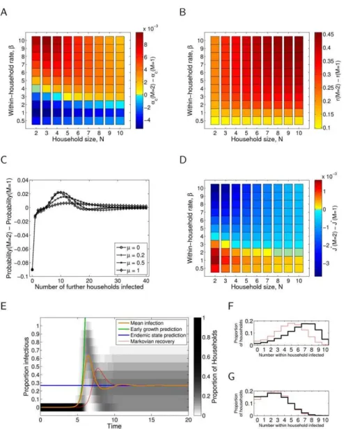
Figure 1 shows the critical level of between-household transmission, ac, required to sustain an epidemic (Plot 1A); the early growth rater(Plot 1B); the offspring distribution (Plot 1C); the endemic prevalence proportionJ(Plot 1D); and the transient dynamics of infection (Plot 1E; see 1F and 1G also), all for the case of exponentially distributed infectious period (M~1). The precise parameter values are provided in the Figure caption; other rate parameter values are presented in the Supporting Information File S1.
Examining the critical level of between-household transmission (Plot 1A) indicates that two factors contribute to the success of an
infection. For large household sizes, the main determinant of epidemic success is whether within-household transmission (governed byb) can produce an epidemic within the household – if it can, then the final size within households is relatively large and so relatively small levels of between-household transmission,
a, can sustain an epidemic. For smaller households of sizeN~2 andN~3, this is not seen, and appreciable between- and within-household transmission is always necessary to sustain an epidemic.
The endemic prevalence of infection (when between-household transmission rate a~1; Plot 1D) is again predominately deter-mined by within-household transmission,b, for larger households, with household size,N, only having a major impact when it is below size4. However, unlike the critical level of transmission (Plot 1A) and early growth rate (Plot 1C), varying the rate of waning immunity, m, has a significant effect in terms of absolute prevalenceJN, which reduces as the rate of loss of immunitym
Figure 1. Epidemiological quantities as defined in the main text for the exponential (M~1) infectious period distribution.(A) Critical transmissionac, with rate of waning immunitym~1. (B) Early growth rater, with rate of waning immunitym~1and between-household transmission parametera~1. (C) Offspring distribution, with within-household transmission rate parameterb~6, house sizeN~10and between-household transmission parametera~1. (D) Endemic infectionJ, with rate of waning immunitym~1and between-household transmission parametera~1. (E) Transient dynamics, with within-household transmission rate parameter b~6, house sizeN~10, rate of waning immunitym~1and between-household transmission parametera~1. (F) As in E at peak prevalence. (G) As in E at endemic prevalence.
is reduced, and vanishes in the absence of waning immunity (m~0); see Supporting Information File S1.
The early growth rater(with between-household transmission
a~1; Plot 1B) varies with both within-household transmission,b, and household size, N, and is only weakly affected by waning immunity,m(see Supporting Information File S1). We observe that the critical between-household transmission rate (Plot 1A) and the endemic prevalence of infection (Plot 1D) show far greater saturation with both household size, N, and within household transmission rate,b, compared to the early growth rate (Plot 1B). This is because the critical transmission rate,ac, and the endemic
prevalence of infection, J, depend on the number of cases produced over one generation (which rapidly saturates as susceptibles within the household get infected), whereas the early growth rate, r, depends on the instantaneous transmission rate
from infected individuals (which is less influenced by households reaching saturation).
The offspring distribution (Plot 1C) shows a significant probability that a newly infected household will fail to infect any further households; often because the infection fails to spread within the household. This failure probability is relatively unaffected by the waning immunity rate,m; whereas increasing
m leads to an increased probability of generating very large numbers of secondary cases. The bimodality of these distributions is a qualitative difference from distributions considered in detail at the individual level [50,51] and therefore can be expected to lead to very different stochastic invasion and persistence properties.
The complete model dynamics at a given parameter set (Plot 1E) demonstrates that our methods for calculating early growth (green line) and the endemic state (blue line) are sound, and also that the
Figure 2. Epidemiological quantities as defined in the main text for the gamma (Mw1) infectious period distribution, compared to the exponential (M~1) results, where within household transmission rate parameter,b, is held constant.(A) Critical transmission differenceDac, with rate of waning immunitym~1;M~2. (B) Early growth rate differenceDr, with rate of waning immunitym~1and between-household transmission parametera~1;M~2. (C) Offspring distribution difference, with within-household transmission rate parameterb~6, house sizeN~10and between-household transmission parametera~1;M~2. (D) Endemic infection differenceDJ, with rate of waning immunitym~1 and between-household transmission parametera~1; M~2. (E) Transient dynamics, with within-household transmission rate parameterb~6, house sizeN~10, rate of waning immunitym~1and between-household transmission parametera~1; M~3; exponential (M~1) results are shown as a thin red line for comparison. (F) As in E at peak prevalence. (G) As in E at endemic prevalence.
proportion of households with a given prevalence assumes a unimodal distribution around the mean, with significant variance. Figures 2 and 3 essentially repeat the evaluation of each of the epidemiologically relevant quantities for the case of gamma distributed infectious period of order Mw1, with b and pheld constant, respectively. In panels (A), (B), (C) and (D) the change in the quantity (respectively, ac, r, probability of offspring number,
andJ) with respect to the assumption of an exponential infectious period has been presented; likewise, in (E), the mean prevalence curve and, in (F) and (G), the full distribution of prevalence, under the assumption of an exponential infectious period have been superimposed for reference.
With respect to the critical transmission rate,ac, the early growth rate,r, and the endemic prevalence of infection,J, it can be seen that both the magnitude and direction of change can differ
depending upon whether the transmission parameter b or the probability of transmission,p, is held constant. With respect to these quantities, holdingpconstant generally results in more significant changes. Furthermore, in general, a higher level of between-household transmission,a, is required to sustain an epidemic, and thus the endemic prevalence of infection,J, witha~1is generally reduced. The early growth rate increases ifbis held constant (Plot 2B) and generally decreases ifpis held constant (Plot 3B).
With respect to the offspring distributions (C), once again the incorporation of gamma-distributed infectious period, and choice of what is held constant between epidemics, has a significant impact. In both cases the probability of no secondary households infected decreases, and by a substantial margin in the case ofbheld constant. In the b constant case the probability of a small number of secondary infections also decreases, whilst in thepconstant case this
Figure 3. Epidemiological quantities as defined in the main text for the gamma (Mw1) infectious period distribution, compared to the exponential (M~1) results, where probability of transmission,p, is held constant.(A) Critical transmission differenceDac, with rate of waning immunitym~1;M~2. (B) Early growth rate differenceDr, with rate of waning immunity m~1and between-household transmission parametera~1;M~2. (C) Offspring distribution difference, with within-household transmission rate parameterb’&3:29(b~6), house sizeN~10 and between-household transmission parameter a~1; M~2. (D) Endemic infection differenceDJ, with rate of waning immunitym~1and between-household transmission parametera~1;M~2. (E) Transient dynamics, with within-household transmission rate parameterb’&2:74(b~6), house sizeN~10, rate of waning immunitym~1and between-household transmission parametera~1; M~3; exponential (M~1) results are shown as a thin red line for comparison. (F) As in E at peak prevalence. (G) As in E at endemic prevalence.
is not seen. In both cases there is a decrease in the tail of the distribution, corresponding to reduced probability of a large number of secondary infections, and the major increase in probability mass occurs in the vicinity of the second peak of the exponential offspring distribution case. Despite these changes, for this parameter set, the bimodal feature of these distributions remains.
Finally, we consider the influence of gamma-distributed infectious period, and what is held constant, by studying the full dynamics of infection. Holdingbconstant (Plot 2E) results in an earlier epidemic with a larger peak infection when compared to the exponential case, whilst holding p constant (Plot 3E) results in an epidemic with similar, but slightly reduced, peak incidence but slower take-off and hence delayed peak. Also interestingly, the incorporation of gamma-distributed infectious period results in a slight oscillatory approach to endemicity, with mean infection dropping below the endemic prevalence following the peak, and slightly overshooting the endemic level again before converging to equilibrium.
Discussion
In this paper, we have focused on appropriate numerical methods for efficient calculation of epidemiologically relevant quantities in households models obeying anSIRSdisease paradigm. Solutions of the kind we have found provide a useful bridge between formal work [36] and individual-based simulation [24], allowing us to study the effects of finite size, stochasticity, and infectious and recovered period distributions at the household level while still in the infinite-size limit at the population level. This has allowed us to quantify some basic behaviours of household structured dynamics; for example the impacts of varying within-household and between-household transmission rates and the role of waning immunity.
In essence the behaviour of the households model can be explained by two different processes. Firstly, compared to purely individual-based transmission (at rate a) the action of within-household transmission (at rate b) is to amplify the infection; so households act as amplifiers for the general transmission process. Secondly, the clustered network structure within a household leads to rapid depletion of the locally susceptible population and hence saturation of amplification effect (and other household properties) as the within-household transmission rate increases. Using our methods, a full sweep of parameter space (as provided in Supporting Information File S1) requires only a few seconds of desktop processor time and so comprehensive sensitivity analysis around a region of parameter space relevant to a given applied problem is also readily obtained. In addition, such methods are able to rapidly calculate likelihood values for any given observations, leading to efficient methods of parameter estimation from household-structured data.
Our results additionally provide one of the first explicit studies of the impact of gamma-distributed infectious periods on dynamics at the household level. Biologically significant effects arise from this change in infectious period distribution, with both the magnitude and direction of these effects varying depending on which parameters are held constant when comparing models. This link between which quantities are observed and therefore which model parameters are held constant, is likely to have significant
impact during the early stages of a disease outbreak in determining an appropriate response.
The methodology used to consider gamma-distributed infec-tious periods can be straightforwardly extended to include latent and prodromal stages of infection. For homogeneously mixed models, the most common such addition is an ‘exposed’ class through which infected individuals pass before becoming fully infectious, leading to the standardSEIRmodel. This does not alter threshold and final size behaviour compared to theSIRmodel, but can cause a highly significant reduction of the early growth rate and modification of other features of the transient dynamics, which we would also expect to see in household models.
We also believe that the epidemiological consequences of the shape of the household offspring distribution warrant further consideration, as has been done for individual-level offspring distributions [50,51]. The ability to construct this distribution through the solution of sets of linear equations offers the possibility of deriving such a distribution, and therefore a greater under-standing of stochastic invasion and persistence, for a range of more complex disease natural histories.
Methodologically, we hope that the reduction of many problems in household epidemic theory to solving a set of linear equations through the theory of path integrals for Markov chains will be of significant use, and have made MATLAB code available to encourage this in the Supporting Information File S2. It is important to note that the consideration of distributions of household sizes is simply done within our framework, but is not included in this work since its main impact is known, from theoretical work, to be on control strategy rather than dynamics. While it could be argued that the methodologies presented here simply allow us to produce the same results more quickly than by using direct integration, numerically efficient algorithms can open up problems to analysis that are currently unsolvable. One example of this would be to consider epidemiological dynamics of sub-populations much larger than households, either ecologically-motivated or as a simplification of large-scale structured models of human and animal disease.
Supporting Information
File S1 Calculation of disease dynamics in a population of households. In this Supporting Information File S1, we include additional technical discussion, and supplementary figures. Found at: doi:10.1371/journal.pone.0009666.s001 (0.08 MB PDF)
File S2 Calculation of disease dynamics in a population of households. In this Supporting Information File S2 we provide MATLAB code.
Found at: doi:10.1371/journal.pone.0009666.s002 (0.01 MB ZIP)
Author Contributions
Conceived and designed the experiments: JR TH MJK. Performed the experiments: JR TH MJK. Analyzed the data: JR TH MJK. Contributed reagents/materials/analysis tools: JR TH MJK. Wrote the paper: JR TH MJK.
References
1. Kermack W, McKendrick A (1927) A contribution to the mathematical theory of epidemics. Proc R Soc Lond A 115: 700–721.
2. Anderson R, May R (1992) Infectious diseases of humans. Oxford: Oxford University Press.
3. Keeling M, Rohani P (2008) Modeling infectious diseases in humans and animals. Princeton: Princeton University Press.
4. Bartlett M (1956) Deterministic and stochastic models for recurrent epidemics. Proc 3rd Berkeley Symp Math Statist Probab 4: 81–109.
5. Bailey N (1957) The mathematical theory of epidemics. London: Griffin. 6. Andersson H, Britton T (2000) Stochastic Epidemic Models and Their
Statistical Analysis. Berlin: Springer Lectures Notes in Statistics, Vol. 151, Springer.
7. Diekmann O, Heesterbeek J (2000) Mathematical Epidemiology of Infectious Diseases Model Building, Analysis and Interpretation. England: Wiley. 8. Altmann M (1995) Susceptible-infectious-recovered epidemic models with
9. Keeling M, Rand D, Morris A (1997) Correlation models for childhood epidemics. Proc R Soc Lond B 264: 1149–1156.
10. Watts D, Strogatz S (1998) Collective dynamics of ‘‘small-world.
11. Keeling M (1999) The effects of local spatial structure on epidemiological invasions. Proc R Soc Lond B 266: 859–867.
12. Potterat J, Rothenberg R, Muth S (1999) Network structural dynamics and infectious disease propagation. Int J STD AIDS 10: 182–185.
13. Klovdahl A (2001) Networks and pathogens. Sex Transm Dis 28: 25–28. 14. Halloran M, Longini I, Nizam A, Yang Y (2002) Containing bioterrorist
smallpox. Science 298: 1428–1432.
15. Keeling M, Eames K (2005) Networks and epidemic models. J Roy Soc Interface 2: 295–307.
16. Boccaletti S, Latora V, Moreno Y, Chavez M, Hwang DU (2006) Complex networks: Structure and dynamics. Physics Reports 424: 175–308.
17. Dangerfield C, Ross J, Keeling M (2009) Integrating stochasticity and network structure into an epidemic model. J Roy Soc Interface 6: 761–774.
18. Ball F (1986) A unified approach to the distribution of total size and total area under the trajectory of infectives in epidemics models. Adv App Prob 18: 289–310.
19. Addy C, Longini Jr. I, Haber M (1991) A generalized stochastic model for the analysis of infectious disease final size data. Biometrics 47: 961–974. 20. Becker N, Dietz K (1995) The effect of household distribution on transmission
and control of highly infectious diseases. Math Biosci 127: 207–219. 21. Ball F, Mollison D, Scalia-Tomba G (1997) Epidemics with two levels of mixing.
Ann App Prob 7: 46–89.
22. Ball F, Neal P (2002) A general model for stochastic sir epidemics with two levels of mixing. Math Biosci 180: 73–102.
23. Cross P, Lloyd-Smith J, Johnson P, Getz W (2005) Duelling timescales of host movement and disease recovery determine invasion of disease in structured populations. Ecol Lett 8: 587–595.
24. Cross P, Johnson P, Lloyd-Smith J, Getz W (2007) Utility ofr0as a predictor of disease invasion in structured populations. J Roy Soc Interface 4: 315–324. 25. House T, Keeling M (2008) Deterministic epidemic models with explicit
household structure. Math Biosci 213: 29–39.
26. Ball F, Sirl D, Trapman P (2009) Threshold behaviour and final outcome of an epidemic on a random network with household structure. Adv App Prob 41: 765–796.
27. Ferguson N, Cummings D, Fraser C, Cajka J, Cooley P, et al. (2006) Strategies for mitigating an influenza pandemic. Nature 442: 448–452.
28. Pellis L, Ferguson N, Fraser C (2009) Threshold parameters for a model of epidemic spread among households and workplaces. J R Soc Interface 40: 979–987.
29. Hufnagel L, Brockmann D, Geisel T (2004) Forecast and control of epidemics in a globalized world. PNAS 101: 15124–15129.
30. Kao R, Danon L, Green D, Kiss I (2006) Demographic structure and pathogen dynamics on the network of livestock movements in great britain. Proc R Soc Lond B 273: 1999–2007.
31. Robinson S, Everett M, Christley R (2007) Recent network evolution increases the potential for large epidemics in the british cattle population. JRS Interface 4: 669–674.
32. Becker N, Utev S (1998) The effect of community structure on the immunity coverage required to prevent epidemics. Math Biosci 147: 23–39.
33. Fraser C (2007) Estimating individual and household reproduction numbers in an emerging epidemic. PLoS ONE 2: e758.
34. Wu J, Riley S, Fraser C, Leung G (2006) Reducing the impact of the next influenza pandemic using household-based public health interventions. PLoS Med 3: e361.
35. House T, Keeling M (2008) Household structure and infectious disease transmission. Epidemiol Infect 137: 654–661.
36. Ball F (1999) Stochastic and deterministic models for sis epidemics among a population partitioned into households. Math Biosci 156: 41–67.
37. Ball F, Lyne O (2001) Stochastic multitype sir epidemics among a population partitioned into households. Adv App Prob 33: 99–123.
38. Koopman J, Chick S, Simon C, Riolo C, Jacquez G (2002) Stochastic effects on endemic infection levels of disseminating versus local contacts. Math Biosci 180: 49–71.
39. Keeling M, Grenfell B (2002) Understanding the persistence of measles: reconciling theory, simulation and observation. Proc R Soc Lond B 269: 335–343.
40. Ross J, Pagendam D, Pollett P (2009) On parameter estimation in population models ii: multi-dimensional processes and transient dynamics. Theor Pop Biol 75: 123–132.
41. Norris J (1997) Markov chains. Cambridge: Cambridge University Press. 42. Pollett P, Stefanov V (2002) Path integrals for continuous-time markov chains.
J App Prob 39: 901–904.
43. Pollett P (2003) Integrals for continuous-time markov chains. Math Biosci 182: 213–225.
44. Daniels H (1967) The distribution of the total size of an epidemic. Proc 5th Berkeley Symp Math Statist Prob 4: 281–293.
45. Goldstein E, Paur K, Fraser C, Kenah E, Wallinga J, et al. (2009) Reproductive numbers, epidemic spread and control in a community of households. Math Biosci 221: 11–25.
46. Ghoshal G, Sander L, Sokolov I (2004) Sis epidemics with household structure: the self-consistent field method. Math Biosci 190: 71–85.
47. Kurtz T (1970) Solutions of ordinary differential equations as limits of pure jump markov processes. Journal of Applied Probability 7: 49–58.
48. Keeling M, Ross J (2008) On methods for studying stochastic disease dynamics. J Roy Soc Interface 5: 171–181.
49. Longini Jr. I, Koopman J, Monto A, Fox J (1982) Estimating household and community transmission parameters for influenza. Am J Epi 115: 736–751. 50. Lloyd-Smith J, Schreiber S, Kopp P, Getz W (2005) Superspreading and the
effect of individual variation on disease emergence. Nature 438: 355–359. 51. James A, Pitchford J, Plank M (2007) An event-based model of superspreading in