www.ann-geophys.net/26/1777/2008/ © European Geosciences Union 2008
Annales
Geophysicae
Equinox transition at the magnetic equator in Africa: analysis of
ESF ionograms
B. J.-P. Adohi1, P. M. Vila2, C. Amory-Mazaudier2, and M. Petitdidier2
1Universit´e de Cocody, Laboratoire de Physique de l’Atmosph`ere, 22 BP 582 Abidjan 22, Ivory Coast
2Centre National de la Recherche Scientifique/Universit´e Versailles Saint-Quentin en Yvelines, Centre d’Etude des Environnements Terrestre et Plan´etaires, 4 avenue de Neptune, 94107 Saint-Maur-des-Foss´es Cedex, France Received: 28 September 2007 – Revised: 17 March 2008 – Accepted: 26 March 2008 – Published: 26 June 2008
Abstract. We study equatorial night-time F layer be-haviour from quarter-hourly ionograms at Korhogo/Ivory Coast (9.2◦N, 5◦W, dip lat. −2.4◦) during local Spring
March–April 1995, declining solar flux period, according to the magnetic activity. The height and thickness of the F-layer are found to vary intensely with time and from one day to the next. At time of the equinox transition, by the end of March, a net change of the nightly height-time variation is observed. The regime of a single height peak phase before 22 March changes to up to three main F-layer height phases after 30 March, each associated to a dominant mechanism. The first phase is identified to the post-sunsetE×B pulse, the second phase associated to a change in the wind circula-tion phenomenon and the third one attributed to pre-sunrise phenomena. The influence of the magnetic activity is iden-tified by the increase in the second peak amplitude. After the 21 April magnetic-equinox period, the height-time mor-phology becomes more irregular suggesting meridional wind abatement. The initiation, the growth and the maintenance of ESF are explored in relation to these nightly variations. The Rayleigh-Taylor instability is clearly identified as main pre-cursor phenomenon. This is followed by the P-type (F-layer peak spread) structures, the whole with no specific depen-dence on the magnetic activity and on the F-layer phases, in contrast to further I and F-type (Inside and Frequency spread) ESFs. We discuss our results in the light of recent advanced experiments in Peru and the pacific.
Keywords. Ionosphere (Equatorial ionosphere; Ionosphere-atmosphere interactions; Ionospheric irregularities)
Correspondence to:C. Amory-Mazaudier ([email protected])
1 Introduction
The Equatorial Spread F layer (ESF) has been documented on low-latitude ionograms since the first Peruvian observa-tions (Booker and Welles, 1938; Cohen and Bowles, 1961). Later Woodman and Lahoz (1976) described the height-time maps of irregularity traces from 50 MHz incoherent scat-ter radar noise at Jicamarca. The clouds, trains and plume shapes at distinctive height levels result from ascending plasma bubbles driven by Rayleigh-Taylor Instability (Os-sakow, 1981). Numerous satellite and radar studies followed (Fejer et al., 1999; Aarons et al., 1996; Mendillo et al., 1997; Basu et al., 1996; Fejer et al., 1979). Using radar obser-vations Tsunoda et al. (1981) and Kudeki et al. (1981) in-terpreted the height-time variation of the middle-scale 2-D structures. The multi-instrument programs of “Guara” cam-paign in Brasil (Pfaff et al., 1997) completed the spectral analysis and dynamics. The Jicamarca Julia-campaign re-sults (Hysell and Burcham, 1998) and the Central Pacific Al-tair results prepared the XXIst Century experiments in the Western Pacific (Fukao et al., 2006; Hysell et al., 2005).
Most of the observations and studies have not concerned African regions. Then African ESF studies published are comparatively few. At the Eritrean subtropics, Wiens et al. (2006) used an advanced all-sky imager and two GPS (Global Positioning System) differential scintillators to de-termine ESF bubble occurrence and zonal drift speeds. Their coverage of both equinoxes during the 2001–2002 solar max-imum provides precious statistics. Farges and Vila (2003) compiled ESF occurrence series obtained from ionograms at Ouagadougou (12.4◦N, 1.4◦W, 1.5◦ dip lat.) and Dakar
(14.8◦N, 17.4◦W, 4.8◦dip lat.) during the year 1995 of
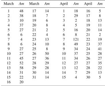
Table 1.Daily Magnetic indexAmfor the period 1 March–30 April.
March Am March Am April Am April Am
1 48 17 14 1 18 16 5
2 38 18 7 2 29 17 8
3 10 19 6 3 2 18 13
4 37 20 8 4 5 19 11
5 27 21 2 5 16 20 14
6 6 22 4 6 8 21 2
7 4 23 13 7 121 22 19
8 6 24 10 8 49 23 37
9 27 25 8 9 34 24 41
10 27 26 50 10 37 25 28
11 45 27 36 11 34 26 27
12 52 28 29 12 27 27 35
13 58 29 28 13 12 28 22
14 31 30 14 14 7 29 13
15 22 31 14 15 4 30 5
16 20
In this paper we describe March and April 1995 results from quarter-hourly IPS 42 ionograms at Korhogo/Ivory Coast (9.2◦N, 5◦W, 2.4◦S dip lat.). They cover the local
spring transition at this near magnetic-equatorial site. In Sect. 2 we present the data set and its processing. Sec-tion 3 is devoted to the time variaSec-tion of the F-layer param-eters around the 1995 spring equinox, and Sect. 4 to an ESF empirical analysis during the same period. Section 5 dis-cusses the equinox transition in West Africa.
2 Data set and processing
The device set up at Korhogo (Ivory Coast) is a vertical sounding IPS 42 transmitter-receiver. The aerial has 80 m width and 25 m height. The power-transmitter pulse is well shaped with 2µs rise time and 10µs width, and the peak power transmitted is 5 kW. The ionosonde explores the HF frequency range [1 MHz–22 MHz]. It records the continuous frequency sweeping echoes reflected at the ground and pro-vides the electron-density profiles of the lower ionosphere in virtual coordinates every 15 min. At low latitudes the se-quences of such profiles give a regular sampling of the F-layer evolution.
Two altitude parameters are commonly determined from the electron-density profiles. The bottom level altitudeh′F
is extrapolated from the low-frequency asymptotic value of the virtual height. The peak level altitudehpF is read on the ordinary trace and is taken as the virtual height for the plasma frequency 0.832foF2, wherefoF2 is the critical fre-quency. The parametersh′F andhpF are estimated every
quarter hour and their plot in the 2-D coordinates system
Fig. 1.ESF occurrence at Korhogo from December 1994 to Decem-ber 1995; the arrow indicates the March–April period investigated in this paper.
(height, time) delimitates the F-layer semi-thickness at any time and allows studying F-layer dynamics.
The iso-frequency lines are inserted betweenh′F andhpF
by simple linear interpolation. When the electron-density profile at any time shows ESF echo, we mark out the fre-quency interval where this echo is observed. We then draw its pattern within the height-time space with the help of the iso-frequency lines. It is very useful for the ESF studies (cf. Sect. 4). The time evolution of such trace allows studying the generation, the development and the propagation of ESF. It particularly helps identifying clear ESF seeding events and some fast increases of the F-layer altitude related to the vari-ety of Rayleigh-Taylor instability regimes.
ESF occurrence was first studied every night over one year, from December 1994 to December 1995. Every quarter-hour, from 18:00 to 06:00 UT, we defined two states. One with ESF-associated echo, quoted 1, and the other for no ESF echo, quoted 0. Note that at Korhogo, UT≈SLT+20 min and in all the paper the time was expressed in UT. Nightly occurrence percentage was then compiled. Figure 1 shows the histogram of ESF occurrence percentage smoothed by running averages over 4 nights. A clear influence of the geographic seasons is exhibited with maximum occurrence ∼80% in spring and autumn periods and only 40% in sum-mer. The data used in this paper are obtained in March and April.
3 Time variation of the F-layer parameters around the spring equinox
3.1 Time dependence of the F-layer height
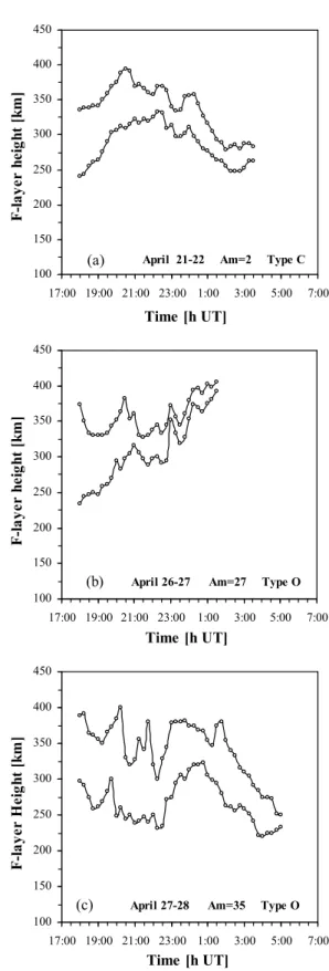
Figure 2 shows the typical time dependences of the layer height registered during all the spring equinox period of March–April 1995.
The lower curve corresponds to the altitude of the bottom of the layerh′F and the upper one to that of the F-layer
max-imum electronic-densityhpF. On 8–9 March (Fig. 2a), a quiet night (Am=6) preceding a period of increasing mag-netic index (Table 1), the F layer height exhibits a single phase of rise (from 18:00 UT to 20:15 UT) and descent (from 20:15 UT to 23:00 UT) of the F-layer. The elevation at the bottom of the layer is about 100 km. During all the rest of the night the height remains constant at about 205 km until sunrise. This is the well-known post-sunset peak (Fejer et al., 1979) usually attributed to theE×Bionospheric electric field pulse.
Figure 2b shows the example of 3–4 April, also a quiet night (Am=2). The variation clearly exhibits a three-phase pattern. Phase 1 is the post-sunset peak described above. Phase 2 occurs between 00:00 UT and 04:00 UT. Its peak is located at about 02:00 UT. The layer goes up from
h′F=215 km toh′F=255 km. The rise and descent have
av-erage velocities of about 16 ms−1and 10 ms−1, respectively. Phase 3 is a pre-sunrise motion starting at about 04:00 UT. Most often in our experiments this phase is not entirely ob-served.
Figure 2c shows the example of 20–21 April, another quiet night (Am=14) preceding a moderately disturbed period. The pattern is a single huge peak extended from 18:00 UT to 03:00 UT. It shows evidence of a three-time motion as fol-lows. A post-sunset rise at about 10 ms−1mean apparent ve-locity takes the bottom of the layer from 245 km at 18:00 UT up to 310 km at 20:00 UT. Then the layer remains practically stationary until 01:00 UT. The descent follows and takes the layer down to 230 km at 02:30 UT with a mean apparent ve-locity of 13 ms−1. The main difference between this profile and the one of 8–9 March (Fig. 2a) is the plateau region be-tween the rise and the descent in 20–21 April (Fig. 2c).
In all the paper the three shapes so described above will be referred as A, B and C for Fig. 2a, b and c, respectively. In other respects, in our set of nightly patterns, few other configurations were observed. They occurred randomly and no similitude could be detected with types A, B and C. We regrouped these particular shapes in the same label O.
! " " #
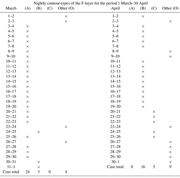
Table 2.Classification of the F-layer profiles according to their nightly patterns for the period 1 March–30 April: Type A corresponds to a single post-sunset peak (Fig. 2a), type B to a three-peak pattern including the post-sunset one (Fig. 2b) and type C to a single huge peak with a plateau region (Fig. 2c). Type O corresponds to undefined, odd profiles.
Nightly contour-types of the F-layer for the period 1 March–30 April
March (A) (B) (C) Other (O) April (A) (B) (C) Other (O)
1–2 × 1–2 ×
2–3 × 2–3 ×
3–4 × 3–4 ×
4–5 × 4–5 ×
5–6 × 5–6 ×
6–7 × 6–7 ×
7–8 × 7–8 ×
8–9 × 8–9 ×
9–10 × 9–10 ×
10–11 × 10–11 ×
11–12 × 11–12 ×
12–13 × 12–13 ×
13–14 × 13–14 ×
14–15 × 14–15 ×
15–16 × 15–16 ×
16–17 × 16–17 ×
17–18 × 17–18 ×
18–19 × 18–19 ×
19–20 × 19–20 ×
20–21 × 20–21 ×
21–22 × 21–22 ×
22–23 × 22–23 ×
23–24 × 23–24 ×
24–25 × 24–25 ×
25–26 × 25–26 ×
26–27 × 26–27 ×
27–28 × 27–28 ×
28–29 × 28–29 ×
29–30 × 29–30 ×
30–31 × 30–1 ×
31–1 × Case total 0 16 5 9
Case total 24 3 0 4
Statistic of the observations over the whole March–April equinox period
(A) (B) (C) Other (O) Number of observations 24 19 5 13 Occurrence (%) 39.3 31.1 8.2 21.3
3.2 Night to night variability of the layer height-An equinox transition
3.2.1 Classification
Table 2 classifies the nightly patterns observed through the equinox period and gives the occurrence percentage of each type.
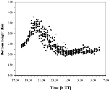
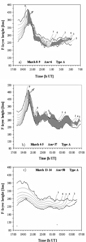
Fig. 3.Night to night variability of the bottom heighth′F of the F2
layer in kilometres (y-axis) as a function of UT time (x-axis), from 6 March to 20 March 1995. The profile exhibits A-type contours.
3.2.2 Type A variation
On Fig. 3 the plot of the bottom heighth′F of the F-layer,
from 6 to 20 March, allows to study the night to night vari-ability of the A-type motion. It is interesting to notice that there is not a strong dispersion ofh′F values in these 15
nights, although the five days, 9 to 14 March, were definitely active. This clearly indicates that the peak of phase 1 is sta-ble and the characteristic parameters of the associated mo-tion do not significantly fluctuate on the successive nights. We find for the velocity values about 14 ms−1at the rise and 10 ms−1at the descent. The peak height is about 330 km and is reached at a characteristic time 20:15 UT.
3.2.3 Type B variation
On Fig. 4 we compare the shapes of the motions for the suc-cessive nights from 30 March to 5 April, a period where the magnetic index varies between 29 and 2 as can be seen in Table 1. Type B patterns dominate. However, the peak of phase 1 is no longer stable as it was the case before the ge-ographic equinox period around 20 March, but shifts along with time as well indicated by the successive positions of the dashed line. On Fig. 4b and d the peak amplitude of phase 2, the F-layer thickness and the bottom heighth′F
are greater than on the other nights (Fig. 4a and c). Dur-ing the nights (1–2 April and 4–5 April) the magnetic ac-tivity presents an important increase that explains the differ-ence, Table 3 providing the three-hourly night-values of the Am index. On 1–2 April (Fig. 4b) the layer extends over more than 110 km with a bottom height about 320 km and on 4–5 April (Fig. 4d), phase 2 contours exhibit a huge peak from 00:00 UT to 05:30 UT with 300 km height and∼70 km
! !
Fig. 4. Night to night variability of the bottom height h′F and
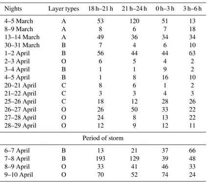
Table 3. Three-hourly magnetic indexAm, for the night plotted in the different figures; the part called “Period of Storm” corresponds to nights not plotted in this paper.
Three-hourly magnetic indexAm
Nights Layer types 18 h–21 h 21 h–24 h 0 h–3 h 3 h–6 h
4–5 March A 53 120 51 13
8–9 March A 8 6 7 18
13–14 March A 49 36 34 34
30–31 March B 7 4 6 10
1–2 April B 56 44 44 63
2–3 April O 6 5 4 2
3–4 April B 1 1 9 2
4–5 April B 1 8 16 10
20–21 April C 8 6 1 2
21–22 April C 3 3 4 3
25–26 April C 18 12 28 26
26–27 April O 26 50 33 22
27–28 April O 24 8 13 22
28–29 April O 12 9 12 11
Period of storm
6–7 April B 13 21 37 66
7–8 April B 193 129 39 48
8–9 April O 33 41 46 33
9–10 April O 70 52 74 24
thickness. In quiet nights, 30–31 March (Fig. 4a) and 3– 4 April (Fig. 4c), its heights and thickness are comparable, ∼260 km and 45 km, respectively.
3.2.4 Type C and O variations
After 21 April, a sudden change from type B to type C clearly appears on Table 2. Figure 5 shows some examples of type C (Fig. 5a) and O (Fig. 5b and c) variations.
During the night 21–22 April (Fig. 5a) of quite magnetic activity (Am=2), the F-layer height varies as a C-type accord-ing to time, with characteristic parameters,∼320 km for the bottom levelh′F,∼40 km for the thickness and∼4 h for the
plateau duration, comparable to that of the night 20–21 April (Fig. 2c) for example.
In 26–27 April (Fig. 5b), the F-layer rises above 400 km after 01:00 UT. The layer density is so reduced that it was not possible to detect it by the ionosonde. The magnetic in-dex is 23, 50 and 33 in the time intervals (18:00–21:00 UT), (21:00–24:00 UT) and (00:00–03:00 UT) respectively. For the following days it is below 15.
In 27–28 April (Fig. 5c), the peak of phase 2 is huge com-pared with that of 4–5 April (Fig. 4d) while the peak of phase 1 usually expected between 18:00 UT and 23:00 UT is inexistent. It appears from Table 2 that, since 21 April, type B is no longer detected. Only types C then O occur.
3.2.5 Conclusion
Whatever the profile of the F-layer parameters, the magnetic-activity increase during nighttime has an impact on their am-plitude. However, it does not modify the variation type, ex-cept in the three cases of O types in April (2–3, 8–9, 9–10).
During the period 30 March–20 April, as shown in Ta-ble 1 and noticed in Sect. 3.2.1, 18 nights out of 21 have a type B variation. The three nights with type O occur after a large disturbed magnetic activity (see Table 3). Unfortu-nately in two nights there are gaps of several hours in the data that preclude detailed analysis. Thus we consider that type B variation is characteristic of the transition period after the spring equinox.
4 Equatorial Spread-F analysis
4.1 Earlier works
gravity waves propagating upward can contribute to ESF ini-tiation (Liao et al., 1989). Evidence of this was shown later (Hysell et al., 1990). The consecutive perturbations at the bottom-side of the F-layer trigger one or more micro-bubbles moving upward which in turn multiply and lead to a large-scale structure that extends to higher altitudes, up to 800 km (Hysell et al., 1998).
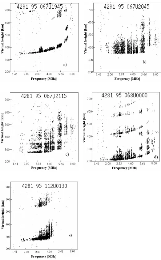
Piggott and Rawer (1972) classified ESF clouds phenom-ena according to their trace morphologies on ionograms. They found two categories. The F-type ESFs (Frequency spread) are irregularity traces parallel to the normal reflec-tion trace. The R-type ESFs (Range spread) are shear-like echoes starting from the F-layer bottom. Since their hand-book publication, new types of ESF have been defined such as the plume rise transient traces.
From coherent scatter radar observations, Hysell et al. (1998, 2002) classified the sequences of a chain of locally-generated ESF events into three categories according to their time position in the chain, their trace morphology, their alti-tude and the physical mechanisms that govern their propaga-tion.
Bottom-type ESF emerges first after sunset, before 21:00 LT. It appears on height-time maps as a relatively thin layer (<50 km thick), near the bottom of the F-layer in the range 250–350 km. It drifts westward, slowly descending. Bottom-type ESF causes very little spread on ionograms.
Bottom-side ESF generally appears after 21:30 LT. Its pat-tern on radar height-time maps is broader (up to 50 km thick) with sometimes very narrow wave-form traces (<5 km wide) that penetrate the topside of the F-layer. This kind of ESF drifts eastward.
Radar plumes are large-scale structures that can extend from 350 km up to 800 km-altitude. They appear in the time interval between the bottom-type and bottom-side ESFs at around 21:00 LT and also drift eastward.
More recently, it has been shown that shear flows in the bottom-side F-layer generate large-scale plasma waves that seed fully-developed ESF (Hysell et al., 2005). The first traces of this phenomenon as observed by UHF/VHF radar are patchy and mainly reside in the valley region although some cases were observed at the bottom of the F-layer be-tween 240 km and 300 km. These low-altitude structures have also been termed bottom-type layers.
ESF may be generated at a location to the west and drifted eastward over the sounding station under the effect of the eastward zonal neutral wind. This travelling irregularity gen-erally appears as patches on a height-time graph and has been observed from digital ionosonde measurements (McDougall et al., 1998).
In the following section we present some examples of ESF traces observed through the March–April period. We de-scribe and characterize the time evolution of the irregulari-ties with respect to the F-layer types. We particularly show that the actual observations correspond to a suite of ESF
Fig. 5.Nightly variations of the bottom heighth′Fand the height of
Fig. 6.ESF behaviour on A-type F-layers for three nights,(a)8–9 March,(b)4–5 March,(c)13–14 March; The X axis corresponds to UT time, the y-axis to the F-layer height in kilometres, the grey area to the ESF pattern, the grey lines to the isofrequency lines (the numbers indicate their values in MHz). The outward arrows direct the development of the P-type ESF and the inward ones indicate immerging clouds.
sequences not all the time identifiable according to the prece-dent classifications.
4.2 ESF in A-type F-layers
Figure 6 presents three examples of ESF behaviour on an A-type F-layer in different magnetic conditions. On these pictures the grey area corresponds to ESF clouds and traces and the curves between h′F and hpF to the iso-density
lines. The numbers indicate the corresponding plasma fre-quency (in MHz). In the quiet night (Am=6) of 8–9 March (Fig. 6a), a clear local seed pattern, ∼5 km thick, arises at about 340 km nearh′Fat 19:45 UT (UT≈SLT+20 min at
Ko-rhogo). It rapidly develops across the whole F-layer as an altitude-extended structure (directed by the outward arrow) reaching the upper limithpF of theE×Bpulse at 20:00 UT. Then it forms a large-scale ESF cloud which fills the early descending F-layer until 21:00 UT. During the descent, the ESF cloud is first tied up to the bottom of the F-layer and is thicker than the initial event (∼25 km thick) until 22:45 UT. It then breaks up into micro-bubbles that progressively dis-appear around 00:00 UT. Another sequence of similar ESF event arises at 01:00 UT without clear seeding phenomenon and disappears at 05:00 UT. This ESF event is unexpected owing to the very low altitude of the F-layer (∼200 km).
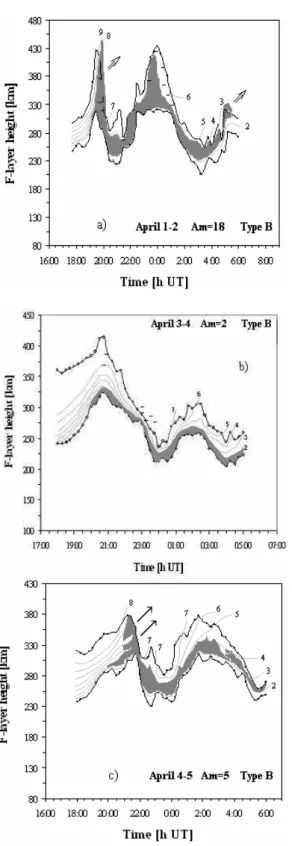
Fig. 8.ESF behaviour on B-type F-layers for three nights,(a)1–2 April,(b)3–4 April and(c)4–5 April. The dashes correspond to the R-type ESF (range-spread) patterns. Note that the transition from the b-type ESF (bottom-spread) to the P-type one (F-layer peak-spread) is abrupt in 1–2 April but progressive in 4–5 April.
extends inside the F-layer. We label this category of echoes I-type ESF (Inside spread) to show that they extend inside the body of the F-layer. Figure 7d also shows a succession of small additional echoes both disposed towards the higher fre-quencies and the higher virtual heights. These echoes appear around 00:00 UT on Fig. 6a, as dispersed micro-structures.
We consider now the night 4–5 March. This night is mag-netically disturbed until 03:00 UT (Table 3). However, until the end of the descent at 21:30 UT, the ESF event (Fig. 6b) is quite similar to that of the quiet night 8–9 March (Fig. 6a) by the initial seeding (b-type echo), the following peak-structure (P-type echo) and the mean-scale inside-extended event (I-type ESF). During the rest of the night, sequences of patches (21:30 UT, 23:15 UT, 00:30 UT) from higher altitudes (as in-dicated by the inward arrow) were found to populate the up-per F-layer. The expected I-type structure is no longer ob-served as was in 8–9 March (Fig. 6a) and ESF cloud rather fills the entire F-layer. The whole oscillates around 280 km until sunrise and ESF disappears upward after 05:00 UT. Fig-ure 6c shows the example of 13–14 March, another disturbed night (Table 3), but with lower altitudes of an A-type contour. Here the peak of theE×B phase is only at a bottom level
h′F∼270 km and ESF logically could not develop. Only
a brief and small patch is observed near the peak, between 19:30 UT and 19:45 UT.
4.3 ESF in B-type F-layers
Figure 8 presents three examples of ESF profile that occur on a B-type F-layer. The night 1–2 April (Fig. 8a) is moderately disturbed (Table 3). The seeding phase of the F-layer peak structure and the following ESF cloud processes are similar to that of 8–9 March (Fig. 6a), despite the different magnetic conditions and F-layer types of these two nights. A local seed pattern arises at about 300 km at 19:30 UT and rapidly gives rise to a P-type ESF trace across the body of the layer with a 80 ms−1average velocity (Fig. 8a). It reaches the upper limit of theE×Bpulse phase at 445 km at 20:00 UT where it de-velops a large ESF cloud across the whole descending layer. At the start of phase 2, about 22:00 UT, ESF is less clearly triggered, but it culminates near 400 km by 23:45 UT after a rapid increase, probably a development into a P-type struc-ture. Then it remains I-type at the descent of the layer until 03:30 UT. Finally, the ESF cloud of phase 3 (cf. Sect. 3.2.3) rises again while the upper half of the layer looses density and ESF vanishes at 04:45 UT. This profile appears as the average well-developed near-magnetic equator ESF.
By contrast, the night 3–4 April is a quiet night and its vari-ation, also a B-type (Fig. 8b), is lacking any seed and peak spread-F traces. Only a weak residual I-type cloud, following
h′F variations and dotted with strata-like patterns (R-type) at
the descent, is visible from 20:15 UT to 05:15 UT.
bottom cloud is duplicated by two rising P-type patterns, re-spectively starting from 300 km and 340 km. From 23:00 UT to 06:00 UT, the F-layer exhibits phase 2 contours. Here the I-type ESF near the peak is at about 300 km-height, high enough to generate a P-type structure as observed af-ter 22:00 UT on 1–2 April (Fig. 8a). This is not the case and ESF behaviour is rather similar to that of 3–4 April (Fig. 8b). 4.4 ESF in C-type F-layers
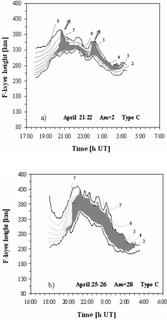
Figure 9 shows two examples of ESF patterns on C-type F-layers, in different magnetic conditions (Am∼2 and 28). In the very quite night (Am∼2) of 21–22 April (Fig. 9a), the initial trace observed around 20:00 UT, slightly above
h′F∼300 km with∼6 km-thickness, compares well with the
local seed pattern shown on the A-type F-layer of 8–9 April (Fig. 6a). However the expected invading cloud that follows arises gradually, in three steps (20:15, 20:30 and 20:45 UT). It reaches the upper limit of the F-layer and disappears up-ward between 20:45 and 21:30 UT as broken clouds (one of the latter can be distinguished at 21:45 UT around 365 km). Along the plateau region, the remaining ESF cloud is thicker, more than 10 km, and stagnates near the bottom limith′F,
suggesting an I-type (Inside spread) structure. It then dis-aggregates into micro-structures as the layer descends be-low 300 km at 23:00 UT as to vanish completely. At that moment a short rise of the bottom layer can be observed acrossh′F=300 km. This appears sufficient to activate
an-other sequence of b-type echo (bottom spread), 5km trace-thickness, which rapidly develops into a P-type one (F-layer peak spread) around 00:00 UT. At the descent of this C-type F-layer the spread structure is first inside the layer un-til 01:15 UT then progressively evolves tied up to the upper limit of the layer as does F-type ESFs (Frequency spread). The ionogram sequence of Fig. 7e is an example of F-type ESF as classified by Pigott et al. (1972). It illustrates the profile structure observed on Fig. 9a between 01:15 and 02:45 UT. Finally, from 02:45 to 03:15 UT ESF breaks into micro-bubbles that disappear upward (Fig. 9a).
In 25–26 April, a moderately disturbed magnetic night, (Fig. 9b), ESF is a b-type trace near h′F=300 km from
19:45 UT to 20:30 UT. A steep rise, with an invading cloud indicating a P-type ESF, reaches 400 km near 20:45 UT (av-erage rise velocity ∼26 ms−1). Then ESF fills the whole layer and lasts along a slow descent, from 21:30 UT to 03:00 UT ath′F=230 km.
4.5 ESF in O-type F-layers
Figure 10 shows three examples of ESF patterns on O-type layers, with different nightly magnetic conditions. The F-layer pattern on 2–3 April, a quiet night (Table 3), is an O-type, with a single peak of phase 1 but continuously decreas-ing from 20:00 UT to 04:00 UT in the pre-sunrise (Fig. 10a). Here no b-type seed and no P-type rise appear. We observe
Fig. 9. ESF behaviour on C-type F-layers for two nights,(a)21– 22 April and(b)25–26 April. The b-type trace is similarly thin in both nights indicating no influence of the magnetic activity on the Rayleigh-Taylor phenomenon. In contrast the I-type trace is thicker in disturbed nights (Fig. 9b) than in quiet nights (Fig. 9a).
only a weak bottom layer cloud descending from 310 km to 280 km between 19:45 UT and 22:00 UT then a residual trace from 340 km to 300 km between 22:15 UT and 23:00 UT. By comparison with the patterns described above these ones seem erratic and likely due to non-local seed source.
Fig. 10.ESF behaviour on O-type F-layers for three nights,(a)2–3 April,(b)26–27 April,(c)28–29 April. On 26–27 April (Fig. 10b) the thin initial trace (b-type echo) indicates a locally generated ESF event. On 2–3 April (Fig. 10a) and 28–29 April (Fig. 10c) the maps exhibit two isolated clouds slowly descending and patchy pat-terns before 22:30 UT respectively, both with evidence of non-local sources.
in an irregular and abnormally rising oscillation motion until 400 km at 01:30 UT.
On 28–29 April, a quiet magnetic night (Table 3), the F-layer pattern begins at 18:00 UT with an unexpected thick plateau region then decreases as in a C-type motion (Fig. 10c). As the usual post-sunset rise does not exist, this layer motion has to be classified as an O-type. As a con-sequence ESF is first dispersed. It starts at h′F=260 km
and shows separate ESF patches peaking at 21:00 UT near
hpF=340 km. The thick F-layer globally shows little con-tour changes until 23:30 UT. However a new start of ESF filling after 23:00 UT seems to be triggered at 22:30 UT. This is the logical consequence of the short increase inh′F from
22:30 UT to 23:15 UT. Then ESF follows the descent of the F-layer and disappears at 02:45 UT under 250 km. From this b-type seed until its end, ESF patterns are quite similar to that of 25–26 April (Fig. 9b).
4.6 Occurrence types complexity
Table 4 summarizes the ESF types of the nights investigated. We notice the frequent succession of b, P and I-types dotted with R-like strata between 20:45 UT and 01:00 UT. At the end of this chain of events, ESF vanishes upward as micro-bubbles. Apart from this category of ESF, others however less frequent, were also observed such as the patch-like struc-ture of 28–29 April between 20:00 and 22:30 UT and the F-type (Frequency spread) echoes generally after the I-type structures. The R and F-type ESFs being the well known range and frequency-spreads already classified (Pigott and Rawer, 1972) only the b, P, I and patch-like structures will be discussed later.
Whatever the F-layer type A, B, C and O, when the night is magnetically quiet, the sequence of ESF after the P-type structure is relatively thin and mainly located at the bottom of the F-layer whereas in perturbed days ESF fills the space between the bottom and maximum heights, above the maxi-mum having no observations. The example of ESF behaviour in the A-type night 13–14 March is not in contradiction to the preceding but confirms earlier observations on the generation of ESF phenomena. Indeed ESF is known to release under the combined effects of the rising speed and the altitude of the bottom level of the F-layer (∼300 km). This was verified in our series and most frequently the seed event is observed while the bottom of the F-layer rises through h′F∼280–
Table 4. ESF sequences observed over the night as a function of the F-layer profiles. The b-type ESFs correspond to small echoes at the bottom of the F-layer (Fig. 7a), the P-type to large-scale structures near the peak of the F-layer (Fig. 7b), the I-type to echoes emerging near the bottom and extending inside the F-layer (Fig. 7d). The R and F-type ESFs are the classical range and frequency spread echoes. The chain of events b, P+R, I+R, F is the most frequently observed.
Nights Layer types ESF types observed
4–5 March A 19 h 45–20 h 45 20 h 45–1 h 30 1 h 30–5 h 5 h–6 h
b, P+R I+R I F
8–9 March A 19 h 45–20 h 45 21 h–23 h 23 h–0 h 0 h 45–3 h 30 5 h–6 h b, P+R I+R Micro-structures (unclassified) I F
13–14 March A 19 h 30–20 h
Patch (unclassified)
1–2 April B 19 h 15–20 h 20 h–23 h 23 h–0 h 30 0 h 30–1 h 30 1 h 30–3 h 30 3 h 30–5 h 30
b, P+R I P+R I+R I F
2–3 April O 19 h 45–22 h 22 h 15–23 h
I Patch (unclassified)
3–4 April B 20 h–0 h 0 h–5 h
I+R I
4–5 April B 20 h–22 h 22 h–5 h 5 h–6 h
b, P I F
21–22 April C 20 h–21 h 30 21 h 30–23 h 30 23 h 30–0 h 15 0 h 15–2 h 2 h–3 h
b, P I b, P I F
25–26 April C 19 h 45–21 h 21 h 30–3 h
b, P I
26–27 April O 20 h 15–21 h 21 h–2 h
b, P I+R
28–29 April O 20 h–22 h 30 22 h 30–0 h 30 0 h 30–2 h 30
Patches (unclassified) b, P I
5 Discussion
5.1 The F-layer profile type
The set of results obtained over the two months investigated suggests 3 different periods.
The A-type profile until 30 March is classically explained by theE×Bdrift that controls the F-layer motion.
Between 30 March and 20 April, the B-type variation is observed. The first phase presents like type A and can be attributed to the E×B drift. The second phase is charac-terized by another peak which presence is not related to the magnetic activity as it also exists on quiet nights. However the amplitude of this second peak increases with increasing magnetic activity. This suggests that other physical processes are involved. A good candidate is the change in wind pat-tern during the equinox period (Roble et al., 1977). During the whole year the dominant wind patterns correspond to the solstice ones with a circulation from the summer hemisphere
to the winter one. The equinox period circulation lasts a few weeks after the equator solar transit as models and observa-tions point out (Roble et al., 1977). This circulation goes from a divergent situation, i.e. from the equator to the poles in each hemisphere on day time and to a convergent one dur-ing night time, the inversion time dependdur-ing on the location. The impact of the wind on the F-layer parameters has been studied since the 60 years and in great details to interpret the thermospheric intertropical arcs at 630 nm (Thuillier et al., 2002). In equinox condition the situation is complex due to the inversion of the meridional wind during nighttime that could explain the second peak. The role of the zonal wind is less important in the African sector as the magnetic declina-tion is close to 0.
two other nights are magnetically disturbed. Several hours after the beginning of a storm or strong magnetic activity, the ionospheric disturbance dynamo process (Blanc and Rich-mond, 1980) affects the wind circulation and associated dy-namo electric fields at low latitudes. Its effect lasts several days. Ionospheric disturbance dynamo is a good candidate for the change from type B to type O observed during 2–3, 8–9 and 9–10 April.
After 20 April until the end of April there is no typical pattern. Type C and type O are both observed with no specific correlation with the magnetic activity.
First, confirming previous schemes by Tsunoda et al. (1981) and Kudeki et al. (1981), Kudeki and Bhat-tacharyya (1999) observed the full distributions of fine-scale post-sunset ion velocity vectors, along the wide plasma vor-tex in the magnetic meridian plane at Jicamarca. They tried to discriminate between the classical scheme and two electro-dynamic extensions of the intertropical sporadic E connected conductors as proposed by H¨arendel et al. (1992) and by Far-ley et al. (1986).
5.2 The ESF events
In this section we discuss our ESF observations and attempt to approach the basic mechanisms involved in the light of theoretical previsions and earlier works above. Most of these works were carried out recently, using advanced techniques (associating coherent backscatter radars, GPS scintillation monitors, sounding rockets. . . ) and numerical modelling, and it is clear that features found under such conditions may not be evident with one-single ionosonde equipment. We can however notice some similarities.
Whatever the magnetic activity, the growth and the main-tenance of ESF phenomenon over our set of nights occur in four sequences, that is, a bottom-spread echo (b-type) around 19:45 UT, followed by a large-scale structure at the peak of the F-layer (P-type event) within the time interval (19:45–20:45 UT), then an inside-extended ESF (I-type) un-til 05:00 UT and finally a frequency-spread (F-type) near sunrise from 05:00 UT to 06:00 UT. This is the scheme most frequently observed on the A and B-type F-layers as clearly illustrated on Table 4. On O and C-types however, the F-layer very often disappears before 04:00 UT leading F-type ESF difficult to be observed.
As already notified the seed phenomenon in local ESF event arises as the bottom limit of the F-layer rises through about 300 km. The chain of events that follows on radar height-time maps is first a thin pattern about 10 km-thick tied up to the bottom limit of the layer and labelled bottom-type ESF. This is followed by a thick layer, upward extended and often reaching higher altitudes of more than 600 km. ESF se-quence after the radar plume is a 40–50 km-thick trace near the bottom of the F-layer, labelled bottom-side ESF.
According to the precedent scheme a local plume genera-tion requires, at least for theE×Bpulse, anh′F peak height
higher than about 300 km. This is likely to be what is ob-served on the A-type F-layers of 4–5 March and 8–9 March, the B-type F-layers of 1–2 April and 4–5 April and the C-type F-layer of 21–22 April and 25–26 April, independently of their magnetic conditions. Indeed, the initial ESF-pattern (the b-type echo) in all these nights is very thin, ∼5–8 km thick, near the bottom limit and similarly rising as is expected for a Rayleigh-Taylor instability trace. The following se-quence (the P-type spread) is thick (more than 80–90 km). It fills the entire F-layer near 21:00 UT and extends until 400– 450 km height. All these characteristics are consistent with bottom-side plumes as visualized and described by Fukao et al. (2004), by means of radar techniques. Our ESF observa-tions also compare well with the features found by Hysell et al. (1998, 2002), by the successive sequences in the whole event and their thickness, the time interval in which they oc-cur and the altitude at the bottom of the F-layer, at least until about 23:00 UT. However in their observations, the precur-sor event and the plume structure for example are westward and eastward respectively. These features are difficult to ac-cess from ionosonde measurements so that we can not con-clude that the thin rising-trace of b-type echo (as detected at 19:45 UT on Fig. 6a) and the following extended pattern of P-type echo are respectively bottom-type ESF and plume structure as defined from radar observations.
Observations by Rodrigues et al. (2004) show that the tran-sition to large-scale plasma bubbles may be either abrupt or progressive. The former is interpreted as an explosion and leads to a steep height-extended pattern whereas the second one gives rise to a bush-like structure. Indeed the 15 min-approximate resolution of our setup is a handicap in fast tran-sient phenomena detection. However a comparison of the P-type event in the 8–9 March night for example to that in 4–5 April exhibits a clear discrimination. The transition is abrupt in the first night. Similar behaviour is also observed in 4–5 March and 1–2 April indicating that the phenomenon is re-current. In contrast, in 4–5 April and 21–22 April a gradual extension in the precursor trace can be distinguished before the P-type events. The preceding means that the transition events so identified are reliable, thus showing similarities with observations by the precedent authors.
Atmosphere Radar (EAR) showing frequent successions of bottom-side patches (at ∼300 km-altitude) travelling east-ward, between 19:30 LT and 22:00 LT. These authors also observed downward-moving plumes, for more than 4 h, from high altitudes to below 300 km. Our observations, on 4–5 March, of succession of downward-moving patches which completely merge into the I-type ESF and fill the whole F-layer at about 300 km between 21:00 UT and 04:00 UT also recall this phenomenon.
Another remark with respect to the seeding phenomenon in the nights investigated in this work is that the probable Rayleigh-Taylor trace arises around a sudden drop of the bot-tom limit of the F-layer as it clearly appears on 25–26 and 26–27 April. This phenomenon is very recurrent and ESF modelling should take it into account.
6 Conclusion
Height-time profiles of the F-layer are analysed based on quarter-hourly ionograms continuously registered at Ko-rhogo/Ivory Coast (9.2◦N, 5◦W, dip lat.−2.4◦) in the
West-African sector during the two-month March–April 1995 pe-riod.
We showed that in addition to the single rise and fall mo-tion generally observed after sunset, others exist depending on the period. Three distinct periods were so identified.
– Before 22 March, only the single rise and fall motion associated to the post-sunset electric field enhancement occurs.
– Between 30 March and 21 April two additional motions occur after the post-sunset one. Both peaks shift along with time and their amplitude increases with increasing magnetic activity.
– After 21 April none of the two precedent profiles ex-ists. The F-layer pattern shows either a single huge peak with a plateau region or an odd profile with no simili-tude with the precedents. The period around 22 March and 21 April being the equinox solar-transit period, the above changes in height-time profiles were identified as an effect of the equinox transition and the additional peaks characterized in the light of actual knowledge on this phenomenon.
ESF patterns were also analysed in the two-months pe-riod according to the F-layer profiles.
– Whatever the equinox period and the F-layer profile the sequence of ESF events until 06:00 UT is b, P+R, I+R and F. Whereas the R and F-type ESFs are the well known range and frequency-spreads already classified in other works (Pigott and Rawer, 1972), the b, P and I-type structures are identified in this paper associating their patterns on height-time graphics and their traces
on ionograms. The seed event, clearly identified, is as-cribed to a Rayleigh-Taylor trace, 5–10 km thick, occur-ring between 280 km and 330 km altitude.
– The Rayleigh-Taylor ESF-trace does not depend on the magnetic activity. In contrast the thickness of the I-type one increases with increasing magnetic activity. The ESF event stops breaking down into upward micro-bubbles.
The main weakness of this work lies in the difficulty to de-termine the peak level altitudehpF of the F-layer with ac-curacy when large-scale ESFs eclipse the ordinary trace of the ionograms. Most time in our experiments this occurs in the time interval [20:30–23:00 UT] around the peak of the
E×Bpulse. In that case the procedure consists in, first re-viewing the consecutive ionograms in that period then reduc-ing the ones with moderate disturbance and at last interpolat-ing the missinterpolat-ing points accordinterpolat-ing to the instructions by Pigott and Rawer (1972). The plot ofhpF vs. time is expected to evolve similarly withh′F in that period as it does in the rest
of the night where the ordinary trace is clearly visible. This allows to check how reliable is thehpF variation pattern in presence of strong ESF and was verified on the height-time profiles studied in this work. Indeed possible errors on that parameter exist and may affect the thickness of the layer in that period but not the time profile.
This work shows evidence of the importance of West African data and should be pursued. For that purpose, net-works of light Doppler-ionosondes and Fabry-Perot Interfer-ometer (FPI) receivers would be the best ground tools for complementing spatial aeronomy and GPS scintillation cam-paigns.
Acknowledgements. The authors thank France-Telecom and the French foreign Ministry for the financial support of the IPS 42 ionosonde. The present series have been available thanks to Emile Kon´e, technical responsible of the Korhogo station. Thanks are also to the University of Cocody (Abidjan Cˆote-d’Ivoire) for its financial support during the training period of Jean-Pierre Adohi at Centre d’´etudes des Environnements Terrestres et Plan´etaires (C.E.T.P/France).
Topical Editor M. Pinnock thanks A. Bhattacharyya and another anonymous referee for their help in evaluating this paper.
References
Aarons, J., Mendillo, M., Yantosca, R., and Kudeki, E.: GPS phase fluctuations in the equatorial region during the MISETA 1994 campaign, J. Geophys. Res., 101(A12), 26 851–26 862, 1996. Basu, S., Kudeki, E., Basu, S., Valladares, C. E., Weber, E. J.,
Blanc M. and Richmond, A.: The ionospheric disturbance dynamo, J. Geophys. Res., 85, 1669–1686, 1980.
Booker, H. G. and Wells, H. W.: Scattering of radio waves by the F-region of the ionosphere, Terr. Magn. Atmos. Electr., 43, 249– 256, 1938.
Cohen, R. and Bowles, K. L.: On the nature of Equatorial Spread-F, J. Geophys. Res., 66(4), 1081–1106, 1961.
Cosgrove, R. B. and Tsunoda, R. T.: Instability of the E-F cou-pled nighttime midlatitude ionosphere, J. Geophys. Res., 109, A04305, doi:10.1029/2003JA010243, 2004.
Farges, T. and Vila, P. M.: Equatorial Spread-F and dynamics in the F-layer over West Africa from ionogram analysis during the declining solar flux year 1994–1995, J. Atmos. Solar Terr. Phys., 65, 1309–1314, 2003.
Farley, D. T., Bonelli, E., Fejer, B. G., and Larsen, M. F.: The pre-reversal enhancement of the zonal electric field in the equatorial ionosphere, J. Geophys. Res., 91, 13 723–13 728, 1986. Fejer, B. G., Farley, D. T., Woodman, R. F., and Calderon, C.:
De-pendence of equatorial F region vertical drifts on season and solar cycle, J. Geophys. Res., 84, 5792–5796, 1979.
Fejer, B. G., Scherliess, L., and de Paula, E. R.: Effects of the vertical plasma drift velocity on the generation and evolution of equatorial spread F, J. Geophys. Res., 104(A9), 19 859–19 870, doi:10.1029/1999JA900271, 1999.
Fukao, S., Ozawa, Y., Yokoyama, T., Yamamoto, M., and Tsun-oda, R. T.: First observations of the spatial structure of F re-gion 3-m-scale field-aligned irregularities with the Equatorial At-mosphere Radar in Indonesia, J. Geophys. Res., 109, A02304, doi:10.1029/2003JA010096, 2004.
Fukao, S. T., Yokoyama, T., Yamamoto, M., Maruyama, T., and Saito, S.: Eastward traverse of equatorial plasma plumes ob-served with the equatorial atmospheric radar in Indonesia, Ann. Geophys., 24, 1411–1418, 2006,
http://www.ann-geophys.net/24/1411/2006/.
Haerendel, G., Eccles, J. V., and Calir, S. C.: Theory for mod-elling the equatorial evening ionosphere and the origin of the shear in the horizontal plasma flow, J. Geophys. Res., 97(A2), 1209–1223, 1992.
Heelis, R. A.: Electrodynamics in the low and middle latitude iono-sphere, a tutorial, J. Atmos. Solar-Terr. Phys., 66, 824–838, 2004. Hysell, D. L., Kelley, M. C., Swartz, W. E., and Woodman, R. F.: Seeding and layering of equatorial spread F by gravity waves, J. Geophys. Res., 95(A10), 17 253–17 260, 1990.
Hysell, D. L. and Burcham, J. D.: JULIA radar studies of equatorial spread F, J. Geophys. Res., 103(A12), 29 155–29 167, 1998. Hysell, D. L. and Burcham, J. D.: Long term studies of equatorial
spread F using the JULIA radar at Jicamarca, J. Atmos. Solar Terr. Phys., 64, 1531–1543, 2002.
Hysell, D. L., Larsen, M. F., Swenson, C. M., Barjatya, A., Wheeler, T. F., Sarango, M. F., Woodman, R. F., and Chau, J. L.: Onset conditions for equatorial spread F determined during EQUIS II, Geophys. Res. Lett., 32, L24104, doi:10.1029/2005GL024743, 2005.
Kudeki, E., Fejer, B. G., Farley, D. T., and Ierkic, H. M.: Inter-ferometer studies of equatorial F region irregularities and drifts, Geophys. Res. Lett., 8(4), 377–388, 1981.
Kudeki, E. and Bhattacharyia, S.: Post sunset vortex in equa-torial F-region plasma drifts and implications for bottom-side spread-F, J. Geophys. Res., 104(A12), 28 163–28 170, doi:10.1029/1998JA900111, 1999.
Liao, C. P., Freidberg, J. P., and Lee, M. C.: Explosive spread F caused by lightning-induced electromagnetic effects, J. Atmos. Terr. Phys., 51(9/10), 751–758, 1989.
MacDougall, J. W., Abdu, M. A., Jayachandran, P. T., Cecile, J. F., and Batista, I. S.: Pre-sunrise spread F at Fortaleza, J. Geophys. Res., 103(A10), 23 415–23 425, 1998.
Mendillo, M., Baumgardner, J., Nottingham, D., Aarons, J., Reinisch, B., Scali, J., and Kelley, M.: Investigation of thermospheric-ionospheric dynamics with 6300A images from the Arecibo observatory, J. Geophys. Res., 102(A4), 7331–7343, 1997.
Ossakow, S. L.: Spread-F theories – a review, J. Atmos Terr. Phys., 43, 437–452, 1981.
Pfaff, R. F., Sobral, J. H. A., Abdu, M. A., Swartz, W. E., Labelle, J. W., Larsen, M. F., Goldberg, R. A., and Schmidlin, F. J.: The Guara campaign: a series of rocket-radar investigations of the earth’s upper atmosphere at the magnetic equator, Geophys. Res. Lett., 24(13), 1663–1666, 1997.
Piggott, W. R. and Rawer, K.: U.R.S.I. Handbook of ionogram in-terpretation and reduction, UAG-23 Report, World Data Centre A, Second Edition, 1972.
Roble, R. G., Dickinson, R. E., and Ridley, E. C.: Seasonal and Solar cycle variations of the zonal mean circulation in the ther-mosphere, J. Geophys. Res., 82(35), 5493–5504, 1977. Rodrigues, F. S., de Paula, E. R., Abdu, M. A., Jardim, A. C.,
Iyer, K. N., Kintner, P. M., and Hysell, D. L.: Equatorial spread F irregularity characteristics over S˜ao Lu´ıs, Brazil, using VHF radar and GPS scintillation techniques, Radio Sci., 39, RS1S31, doi:10.1029/2002RS002826, 2004.
Sastri, J. H., Abdu, M. A., Batista, I. S., and Sobral, J. H. A.: On-set conditions of equatorial (range) spread F at Fortaleza, Brazil, during the June solstice, J. Geophys. Res., 102(A11), 24 013– 24 021, 1997.
Thuillier, G., Wiens, R. H., Shepherd, G. G., and Roble, R. G.: Photochemistry and dynamics in thermospheric intertropical arcs measured by the WIND imaging interferometer on board UARS: A comparison with TIE-CGM simulations, J. Atmos. Solar-Terr. Phys., 64, 405–415, 2002.
Tsunoda, R. T., Livingstone, R. C., and Rino, C. L.: Evidence of a velocity shear in bulk plasma motion associated with the post-sunset rise of the equatorial F layer, Geophys. Res. Lett., 8, 807– 810, 1981.
Wiens, R. H., Ledvina, B. M., Kintner, P. M., Afeverki, M., and Mulugheta, Z.: Equatorial plasma bubbles in the ionosphere over Eritrea: Occurrence and drift speed, Ann. Geophys., 24, 1443– 1453, 2006,
http://www.ann-geophys.net/24/1443/2006/.