Paleoclimatic reconstructions in Western Canada from subsurface temperatures: consideration of groundwater flow

(1)

CPD

1, 93–120, 2005

Paleoclimatic reconstructions in

Western Canada

J. Majorowicz et al.

Title Page

Abstract Introduction

Conclusions References

Tables Figures

◭ ◮

Back Close

Full Screen / Esc

Print Version

Interactive Discussion

EGU Climate of the Past Discussions, 1, 93–120, 2005

www.climate-of-the-past.net/cpd/1/93/ SRef-ID: 1814-9359/cpd/2005-1-93 European Geosciences Union

Climate of the Past Discussions

Climate of the Past Discussionsis the access reviewed discussion forum ofClimate of the Past

Paleoclimatic reconstructions in Western

Canada from subsurface temperatures:

consideration of groundwater flow

J. Majorowicz1,2, S. Grasby3, G. Ferguson4, J. Safanda5, and W. Skinner6

1

Northern Geothermal, 105 Carlson Close, Edmonton, Alberta, T6R 2J8, Canada

2

University of North Dakota, Northern Plains Climate Research Centre, Grand Forks, USA

3

Geological Survey of Canada, Calgary, Canada

4

Department of Earth Sciences, St. Francis Xavier University, Antigonish, Nova Scotia, Canada

5

Geophysical Institute, Prague, Czech Republic

6

Environment Canada, Downsview, Ontario, Canada

Received: 15 June 2005 – Accepted: 25 July 2005 – Published: 9 August 2005 Correspondence to: J. Majorowicz (majorowicz@shaw.ca)

(2)

CPD

1, 93–120, 2005

Western Canada

Title Page

Tables Figures

◭ ◮

Back Close

Full Screen / Esc

Print Version

EGU

Abstract

The surface temperature forcing is responsible for the majority of the observed

devi-ation of temperature with depth. In some cases, differences higher than the error of

measurements are observed between the model and measurements. These can be an indication that other factors than surface temperature change influence subsurface

5

temperature. Groundwater flow is one of the possible candidates.

1. Introduction

The primary assumption of borehole paleoclimatology (Lachenbruch and Marshall, 1986) is that heat transfer is by conduction only. This assumption is justified in areas with negligible vertical movement of underground water (Kane et al., 2001).

Ground-10

water flow is often neglected in GST reconstructions without adequate justification ac-cording to recent studies of Reiter (2005) and Ferguson and Woodbury (2005). In this paper we analyze temperature-depth profiles from the Western Canadian Sedimentary Basin with special focus on the Paskapoo Formation in the Alberta Basin.

The past changes in the energy balance at the Earth’s surface propagate into the

15

subsurface and appear as perturbations of the subsurface thermal regime. Due to

the low thermal diffusivity of rocks, GST changes propagate downward slowly and are

recorded as transient perturbations to the steady state temperature field. Temperature profiles measured in a borehole a few hundred metres deep may contain information about GST changes in the last millennium. This gives us an opportunity to reconstruct

20

surface temperature history by inversion of the temperatureT vs. depthzprofile (T−z).

The result is considered to be a climate record with a secular length proportional to depth of the borehole temperature measurement.

In general, mean annual ground surface temperature tracks the mean annual surface air temperatures taken at screen height (1.5 m above the surface of the ground), in the

25

(3)

Majorow-CPD

1, 93–120, 2005

Western Canada

Title Page

Tables Figures

◭ ◮

Back Close

Full Screen / Esc

Print Version

EGU icz and Skinner, 1997). However, the coherence between ground surface temperature

(GST) warming reconstructed from boreholeT−z profiles and surface air temperature

(SAT) warming has been questioned by Mann and Schmidt (2003) who argued that the ground does not “see” much of the cold winter air cooling in the presence of snow cover because of insulation and reflection of incoming radiation, resulting in potential

5

loss of information of cold-season temperature variations in the reconstructed GST history. The GST annual means are usually higher than the SAT annual means as the snow cover warms the surface (Lachenbruch, 1994; Schmidt et al., 2001; Stieglitz et

al., 2003). The magnitude of the difference between the mean annual ground surface

and surface air temperatures depends on snow cover or the content of soil moisture

10

at the beginning of the freezing season. If these departures between ground and air temperatures change randomly from year to year and their mean values do not change on the time scale of the GST history reconstruction, than the present interpretation of the GST history as a first order estimate of the air temperature history is correct (Putnam and Chapman, 1996; Cermak et al., 2003, Beltrami, 2001; Schmidt et al.,

15

2001; Gonzalez-Rouco et al., 2003). Modelling done by Gonzalez-Rouco et al. (2003) shows that at long time scales terrestrial deep annual soil temperature changes are a good proxy for annual surface air temperature (SAT), and their variations are almost indistinguishable from each other.

Factors like deforestation or forest fires can also significantly change surface

temper-20

ature and influence underground temperature regimes (Majorowicz and Skinner, 1997; Lewis and Skinner, 2003; Skinner and Majorowicz, 1999). Such changes of the land surface are sometimes not well known and their contribution to the warming/cooling of the surface are not easily separated from the irradiative forcing. This is similar to the

influence of groundwater flow uponT−z. These effects are difficult to separate from the

25

e_ffects of surface warming onT−z curvature (Reiter, 2005; Ferguson and Woodbury,

2005). All of these (surface warming due to climatic change, changes related to land

use, hydrodynamic effects etc.) can influenceT vs.z.

(4)

CPD

1, 93–120, 2005

Western Canada

Title Page

Tables Figures

◭ ◮

Back Close

Full Screen / Esc

Print Version

EGU 1D conductive assumption can be discerned in the multi-decadal/century time scale,

GST histories derived from well temperatures over the past several centuries may be much more believable.

We can test the above by comparing measured transient temperature-depth profiles

(T−z) with simulated profiles from the surface air temperature SAT data of nearby

cli-5

mate stations. In this paper we report results of temperature (T) measurements with

depth (z) for borehole sites located in the Western Canadian Sedimentary basin, with

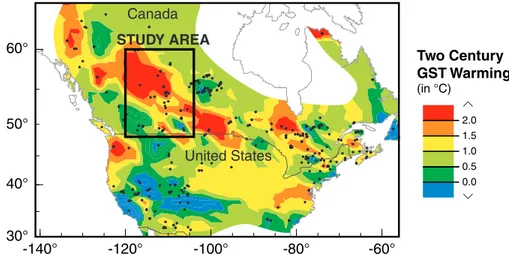
special focus on the Paskapoo Formation in western Alberta. The Mid-west of North America (northern Great Plains in the USA and Western Canadian Prairies) has been experiencing one of the highest mean annual surface air and ground warming in the

10

Northern hemisphere, characterized by a GST warming magnitude of₊2◦_{C over some}

two centuries (Fig. 1; Skinner and Majorowicz, 1999; Gosnold et al., 1997).

2. Paskapoo Formation

The Paskapoo Formation is a mudstone dominated non-marine unit with a series of interbedded sand channels which can form isolated aquifer units. Channel sandstone

15

beds range up to 15 m, but are typically 5–10 m thick. Sand channels are lenticular and can pinch out laterally over short distances (100–150 m or more). However basal sand units can intercalate to form more extensive sheet sands. Sand units have a dominant intergranular porosity with a range from 5 to 30%, and averaging 19% over

the formation. Sandstone permeability’s are typically very low (average 10−14

m2) with

20

the exception of basal coarse-grained sand units (∼10−12m2). Limited paleocurrent

data suggests a general northeastward trend to channel sands suggesting that aquifer units within the Paskapoo have greater continuity on average along that orientation.

The fluvial sandstones of the Paskapoo are interbedded with light grey to greenish or brownish, sandy siltstone and. These fine grained facies form intervals several to

25

several tens of metres thick between the major sandstone horizons and likely act as

(5)

CPD

1, 93–120, 2005

Western Canada

Title Page

Tables Figures

◭ ◮

Back Close

Full Screen / Esc

Print Version

EGU

3. Data

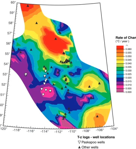
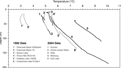
Temperature logs were taken in 51 wells through the prairies (Fig. 2) using portable logging equipment with a thermistor probe. The location of wells logged within the Paskapoo area is shown in Fig. 2. Paskapoo well logs are shown in Fig. 3. Locations of other wells with temperature logs are also shown in Fig. 2. Temperature measurements

5

were made between 1991–1995 and as recently as 2004. The temperature- depth data were used to infer magnitude of recent ground surface temperature (GST) warm-ing (1920–1990 A.D) uswarm-ing the approach described in Majorowicz et al. (2002). The contour map presented in Fig. 2 shows large variability of warming rates. In the region

underlain by the Paskapoo Formation warming rates vary in the 0.005–0.025◦C/year

10

range. A warming rate as high as 0.060◦_{C/year is observed in the north-eastern part}

of the Prairie Provinces.

Temperature measurements were made with a thermistor probe calibrated to 0.01◦C

(relative change) and 0.03◦_{C (absolute change). The probe was attached to 500 m}

ca-ble on a portaca-ble, manually operated winch. The measurements were taken at discrete

15

intervals (2 m and 5 m for the oldest log) in observational wells with no disturbances for decades. These wells monitor piezometric water levels only and no other activi-ties were present after well drilling ceased (before 1980). This ensures that thermal equilibrium exists between water in the well and the surrounding rock mass. Usu-ally, logging of temperature is done at depths below 20 m as the static water level in

20

the wells are well below the surface. In some cases shallower levels were measured (Fig. 3). Above 15–20 m, daily to seasonal temperature changes has been influencing soil temperatures. That upper part of the cased well above the water level is air. The small diameter of the wells relative to their length disallowed any convection in the well bore significant enough to disturb the thermal regime (Jessop, 1990). Nevertheless,

25

(6)

in-CPD

1, 93–120, 2005

Western Canada

Title Page

Tables Figures

◭ ◮

Back Close

Full Screen / Esc

Print Version

EGU duced circulation). Variations of static water level (piezometric surface variations) are

constant and can be between meters to tens of meters seasonally and over longer terms.

Rock chip and well log derived net rock lithology and rock conductivities of the West-ern Canadian Sedimentary Basin (Beach et al., 1987; Jessop, 1990) were used in

5

thermal conductivity estimate. Details of conductivity variation with depth were shown in Majorowicz et al. (1999).

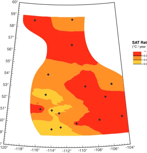
Meteorological data (SAT series) like the one illustrated in Fig. 4, from 22 Environ-ment Canada SAT stations, were used in calculations of SAT warming rates for the 1920–1990 AD (Fig. 5). These are much less variable than the GST rates calculated

10

from well temperature logs (Fig. 2). However, a trend of lower warming rate towards the south-western Rocky Mountain Foothills is apparent in both maps (Figs. 2 and 5). SAT series are also useful in the calculation of the synthetic response below the ground surface that can be compared with temperature transients from temperature logs in wells.

15

Surface air temperature data come from the Canadian historical climate network database (Vincent and Gullett, 1999; Vincent, 1998; Zhang et al., 2000 and the re-cent Environment Canada web based updates). Historical SAT data represent mea-surements originally made at airports, agricultural stations and rural volunteer sites. Instrument compounds are located over grassed surfaces in order to maintain

na-20

tional observing consistency. The calculated mean annual SAT warming magnitudes

for the period 1892 to 1992 varies between 0.3◦ and 1.8◦C across Canada

(Environ-ment Canada, 1995). Recent temperature increases have been neither spatially nor temporally uniform (Zhang et al., 2000).

4. Modelling of surface temperature change effect uponT(z)– The method

25

The reconstruction of the GST history is for time interval [t0tot1] from the subsurface

(7)

CPD

1, 93–120, 2005

Western Canada

Title Page

Tables Figures

◭ ◮

Back Close

Full Screen / Esc

Print Version

EGU

implicitly requires that the perturbations inT(z, t) caused by the GST variation before

timet0 cannot be distinguished from the steady-state field within the depth interval [0,

z_b] at timet1. This requirement can be satisfied by consideringt0sufficiently far away

fromt1.

The GST change will produce a disturbance to a linear portion of the well

temper-5

ature profile assuming constant conductivity K and diffusivity a. The linear portion of

the well temperature profile represents steady flow of heatQfrom the earth’s interior

according to Fourier relation:

Q=−K Go,

whereK is thermal conductivity andG_ois thermal gradient.

10

Extrapolation of the linear portion of thermal profile controlled by deep heat flowQ

and thermal conductivityK to the surfacez_oyields the intercept temperatureT(z_o). The

deviation of the measured temperature profileT(z) from the extrapolated linear profile

results in temperature anomalyDT(z), which in the simplest interpretation represents

the response of the ground to recent rise of the mean annual surface temperature from

15

a previous long-term valueT(z_o) (positive anomaly values) or recent cooling (in case

of negative anomaly). The combination of subsequent warming and cooling events complicates the disturbing signal with depth.

Inhomogeneities in rock properties and three dimensional effects limit resolution of

the details ofT(z, t), where t is time, however, a one dimensional model is capable

20

of resolving the general magnitude of recent temperature changes and timing of its

onset. In the simple one dimensional transient model of the effects of surface GST

change upon temperature depth, the assumption of homogenous sub-surface media is a simplification. Temperature change with depth and time can be written as:

T(z, t)=T(z_o)+G_oz+DT(z, t),

25

whereDT(z, t) represents the response of the ground to recent mean annual

(8)

CPD

1, 93–120, 2005

Western Canada

Title Page

Tables Figures

◭ ◮

Back Close

Full Screen / Esc

Print Version

EGU

governed by the differential equation

d2DT(z, t)/d z2=1/kd T/d t ,

wherek=K/ρ cis thermal diffusivity,ρis density andcis heat capacity.

We can simulate the transient subsurface temperature changes caused by the ground surface temperature variations by using the SAT series under the assumption

5

that the mean difference between the ground and air temperatures is constant through

time. We consider annual meansT i of the SAT as a ground surface forcing function.

POM (pre-observational mean) surface temperature needs to be assumed.

The forcing function consisted of a series ofN jumps of amplitude∆T i=T i−T i−1 at

timesti before the borehole temperature measurement. The subsurface temperature

10

responseT to this forcing at depthz was (Carslaw and Jaeger, 1959)

T(z)=

N X

i=1

∆T i×erf c(z/ p

4kti),

wherek is thermal diffusivity anderf c is the complementary error function. This

cal-culation depends on one free parameter, the mean long-term temperature T_o before

the first change at timet1. ParameterTo is the pre-observational mean (POM).

15

5. Results of paleoclimatic model

The 2004 transient components in the deepest Paskapoo Formation borehole,

War-burg (Fig. 3), has been obtained as (i) a posteriori FSI transients fromT−z logs

(Func-tional Space Inversion; see Shen and Beck, 1991 for method’s description) and (ii) synthetic transients based on SAT time series and assumed POM temperature level

20

for the nearby Calmar meteorological station run by Environment Canada (Fig. 4).

A comparison of the 2004 transient component of T−z in the borehole Warburg

(9)

CPD

1, 93–120, 2005

Western Canada

Title Page

Tables Figures

◭ ◮

Back Close

Full Screen / Esc

Print Version

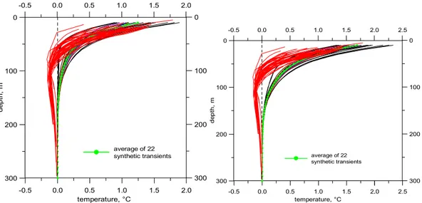
EGU SAT series from Calmar (Fig. 4) is shown in Figs. 6a and 6b. The synthetic curves were

calculated for three values of the POM:

1. POM equal to the 1895–1910 mean;

2. POM 0.5◦C higher than the above mean;

3. POM 0.5◦_{C lower than the mean.}

5

The SAT data cover the period 1915–2003, their mean value is 2.3◦C. The mean of

the first decade 1915–1924 is 1.55◦C. The “boxcar” period is 1790–1910. The SAT

value considered for the gap 1910–1915 is estimated in the same way as in previous

calculations and amounts to 1.1◦C. There are two free parameters – a long-term mean

prior 1790, which is referred to as POM, and the boxcar temperature between 1790

10

and 1910. The considered POM values are centered ±0.5◦C around the mean of

the first observational decade 1915–1924 and attain 1.1◦C, 1.6◦C and 2.1◦C. These

values were combined with the boxcar temperatures 0.6◦C and 1.1◦C. In the case of

POM=1.1◦_{C, only the boxcar value of 0.6}◦_{C was considered.}

Thermal diffusivity used in calculating the synthetic curves was the same as for the

15

FSI, this means 0.7×10−6m2.s−1in the case of Warburg.

There could be several possible sources of the observed disagreement between the synthetic and FSI transient in Fig. 6a. One of them is a problem with short boreholes, where the FSI does not reproduce fully the recent warming. The FSI inversion scheme estimates the undisturbed basal heat flow, and therefore the transient component, by

20

considering in its probabilistic model the whole temperature log. In the case of shallow boreholes it can result in a basal heat flow estimate lower than indicated by a gradient of the lowermost part of the log. One of the results would be a spurious minimum of the GST history, frequently observed in the reconstructions of wells shallower than 150 m (see simulations of the synthetic GST histories in Fig. 4 of Majorowicz et al., 2002) and

25

(10)

CPD

1, 93–120, 2005

Western Canada

Title Page

Tables Figures

◭ ◮

Back Close

Full Screen / Esc

Print Version

EGU Tentatively, we tried to correct the above disagreement between transients by fitting

the lowermost part of a posteriori FSI transients in Fig. 6a to a line and by calculating

new transients as the difference of the old ones and the fitted lines. The resulting curve

is shown by the dashed line and marked as corrected FSI (Fig. 6b). One can see that the degree of coincidence is appreciably better that in the case of the uncorrected

5

one. The corrected FSI transients indicate that the POM is 0 to−0.5◦C lower that the

1895–1910 means for the nearby Calmar SAT station.

Observed cooling at depth below ca. 100 m (Fig. 6a) may correspond to the cold

period during the 1800’s experienced in the prairies, but this is difficult to prove due

to the lack of instrumental data before the 20th century. The transient component of

10

the Warburg’sT−zlog agrees with the GST low before recent warming showed in the

upper ∼80 m of the T−z transient anomaly. Such temperature lows in the late 18th

and all of the 19th century, preceding 20th century warming, explains the negative

slope of theT−z transient from measured logs well (Majorowicz et al., 1999 and this

paper, Fig. 6c). These lows are confirmed by recent tree ring reconstruction done in

15

the Alberta Rocky Mountains (Luckman et al., 1997; Luckman and Wilson, 2005). One additional possible explanation of the disagreement between transient based on SAT-POM forcing models and measured transient below ca. 80 m is downward flow of groundwater. It will be discussed later in the paper.

The above modelling shows that fit between the simulated and observed temperature

20

transient can be hardly a test of GST versus SAT coupling by itself.

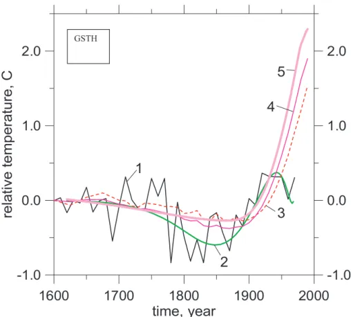
Synthetic curves were also calculated for the Calgary SAT station for several years of the last decade (Fig. 7). A model of SAT-POM – equal to the 1895–1910 mean was

used as forcing. The thermal diffusivity used in calculating the synthetic curves was

the same as for the FSI’s, i.e. 1.0×10−6m2.s−1. We have used the thermal conductivity

25

model based on lithology description and literature (Jessop, 1990) assumed thermal

conductivities and specific heat of 2MJ/(K.m3).

(11)

CPD

1, 93–120, 2005

Western Canada

Title Page

Tables Figures

◭ ◮

Back Close

Full Screen / Esc

Print Version

EGU with transients calculated from FSI’s of temperature logs in all 51 wells (locations in

Fig. 2) show significant difference below 70–80 m depth (Figs. 8a and 8b) depending

on the assumed POM. Differences above the errors of measurement are in the 70–

200 m depth range. The simplification of the model used in the simulations is that POM is an assumed quantity.

5

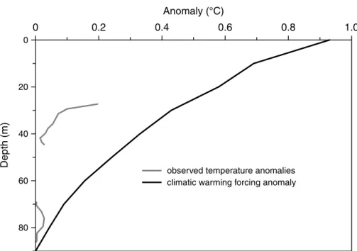
Comparison of the simulatedT−zanomaly from SAT-POM model for Calgary (Fig. 9)

can be also compared with measurements ofT−zin one location in Airdrie (Paskapoo

Fm). Deep regional geothermal gradient (25 mK/m) and regional steady state surface

temperature 4◦C were used to exctract theT−z anomaly. In this case it is apparent

thatT−zbased on Calgary station SAT forcing is much higher than the observedT−z.

10

Two explanations can be given: (1) SAT in Calgary is subject to a “city island” warming

effect; (2) changes in surface recharge and water flow disturbed the AirdrieT−z.

The above comparisons show that the observed changes in temperature-depth are only partly explained by the assumed SAT-POM forcing model.

6. Groundwater flow consideration

15

One of the well known possible causes of observed changes in the temperature-depth curve is downward water flow. The typical profile associated with downward flowing groundwater creates a lower downward curvature (Bredehoeft and Papadopulos, 1965; Reiter, 2005). This tends to show up as recent warming in the upper part of the profile and cooling at depth when reduced, assuming that the temperature profile can be

de-20

scribed byT(z, t)=T(z_o)+G_oz+∆T(z, t), which neglects advective heat flow. The type of perturbation that would be associated with downward flow of groundwater depends on recharge rates, depth and time.

(12)

CPD

1, 93–120, 2005

Western Canada

Title Page

Tables Figures

◭ ◮

Back Close

Full Screen / Esc

Print Version

EGU ground water in one dimension for a homogeneous and isotropic porous medium:

κ_e∂

2

T

∂z2 −cfρf

∂(vzT)

∂z =csatρsat ∂T

∂t ,

whereκ_e is thermal conductivity,T is temperature,c_f is the specific heat of water,ρ_f

is the density of water, v_z is specific discharge, c_sat is the specific heat capacity of

the saturated porous medium andρsatis the density of the saturated porous medium.

5

In the current study, this equation is solved numerically using MULTIFLO (Painter and

Seth, 2003), which utilizes an integrated finite difference formulation.

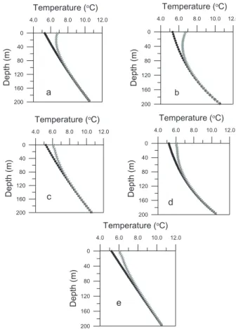
The results of the advective-conductive models assuming groundwater recharge rates of 25 and 100 mm/yr were calculated in this paper for Calgary and Calmar stations assuming SAT records as forcing (Fig. 10). The method described in detail by Ferguson

10

and Woodbury (2005) was used. We have estimated the approximate surface temper-ature to which the SAT anomalies are added or subtracted from by extrapolating the

Airdrie and Calmar profiles to the surface, (5.2 and 5.3◦C, respectively). We have used

a fixed temperature at the bottom of the aquifer and fixed pressure boundary condition.

In both cases we have used a temperature of 10.6◦C at the base of the model at 200 m,

15

based on an extrapolation of the Warburg log. These models are by no means perfect because we know little about the seepage velocities of water over the broader area, and there is most likely horizontal flow of groundwater that should be considered as well. Recent estimates for long term recharge rates into the Paskapoo Formation in

the Spyhill area north of Calgary suggest minimal recharge rates (∼5 mm/yr, T, Van

20

Dijk, pers. com., 2005). In case of 5 mm/year modelT−z shows no curvature.

While the high end recharge rate used here suggests that for the extreme case some of the observed curvature in the profiles, especially the Warburg profile, could be due to groundwater flow, it is more likely that the low recharge rates in this semi-arid region would have minimal impact. Another issue is that this assumes steady-state fluid flow,

25

(13)

CPD

1, 93–120, 2005

Western Canada

Title Page

Tables Figures

◭ ◮

Back Close

Full Screen / Esc

Print Version

EGU

7. Discussion and conclusions

Modelling and observations presented above show that differences higher than the

error of measurement are observed between the model based on surface forcing (ob-served SAT plus assumed POM) and observation. It is mainly due to our poor knowl-edge of the climatic history before the observational period and poor knowlknowl-edge of

5

other factors like groundwater flow, snow cover trends etc. These factors are difficult

to distinguish from each other without additional independent information about the climate preceding the observational SAT record.

The transients shown here for all of Alberta and S. Saskatchewan (51 wells) and transients modeled here for 22 SAT stations (Figs. 8a and 8b) agree well with the

ex-10

ample analyzed for the Paskapoo Fm well in Warburg (Fig. 6a) despite that the majority of wells are outside the area of Paskapoo. There are only 11 Paskapoo logs available

(Fig. 3). Significant disagreement exists between modeled transients ofT−zSAT-POM

models and transients based on measured T−z profiles. The disagreement is most

significant in the 70–200 m depth interval.

15

A “Box-car” model approximating lower temperature in 1800’s preceding 20th cen-tury warming used by Majorowicz et al. (1999) and this paper (Fig. 6c) can explain the observed discrepancy and model the observed negative slope of temperature tran-sients below 80 m depth. While the observed cooling at this depth may correspond to

the cold period during the 1800’s experienced in the prairies, it is difficult to prove due

20

to the lack of instrumental data. There is support of the above explanations in proxy record from tree rings in the Alberta Rocky Mountain’s Colombia glacier region (Luck-man et al., 1997; Luck(Luck-man and Wilson, 2005). A temperature low of the late 1700s through 1800’s is apparent from the tree ring based temperature history reconstruction of Luckman et al. (1997) as shown in Fig. 11.

25

The groundwater flow as another possible explanation was also examined.

Down-ward groundwater flow creates T−z curvature and this tends to show up as recent

(14)

CPD

1, 93–120, 2005

Western Canada

Title Page

Tables Figures

◭ ◮

Back Close

Full Screen / Esc

Print Version

EGU proxy SAT reconstructions indicate that 1800 s cooling was present and this would be

enough to explainT−z observations If this is the case, it would be consistent with

re-cent work suggesting long term recharge rates are significantly lower than the modeled 100 mm/year. Even models using recharge rates (25 mm/yr) at five times the estimated

average values do not show evidence for groundwater flow affecting the temperature

5

profile. Thus the temperature-depth curve in this region can be explained to a large extend by surface cooling/warming models alone, without assumption of significant ad-vective heat transport.

It is also to be remembered that the solution of the problem is not unique and FSI seeks the most probable solution within its probabilistic model.

10

While, most of the observed transients can be explained by surface temperature change, the deviation of the transients from well temperature logs from the synthetic transients based on SAT-POM model exists. Assuming lower POM’s will make that

di_fference even larger. However, the assumed POM constant level of temperature

before the start of observations in the early 20th century may not be valid and the local

15

19th century surface temperature low related to Little Ice Age could explain observed temperature’s transient (Majorowicz et al., 1999).

The results show that SAT forcing is the main driving factor for the underground

temperature changes diffusing with depth. It supports validity of borehole temperature

paleoclimatology hypothesis that the ground surface temperature is systematically

cou-20

pled with the air temperature in longer term (decades). The analysis of the transient temperatures with depth presented here also supports the validity of the assumption

that the changes in ground surface temperature di_ffuses mainly by conduction into

the subsurface and impose a transient “climate” signal on the steady-state geother-mal gradient. These assumptions are limited to the sites in which no hydrogeological

25

disturbance or land surface changes were observed.

Acknowledgements. We would like to thank Environment Alberta and Saskatoon Research

(15)

CPD

1, 93–120, 2005

Western Canada

Title Page

Tables Figures

◭ ◮

Back Close

Full Screen / Esc

Print Version

EGU

logging of temperature.

This material is partially based upon work supported by the GSC Calgary, EC Downsview and the National Science Foundation under Grant No. 0318384.

References

Baker, D. G. and Ruschy, D. L.: recent warming in eastern Minnesota shown by ground tem-5

peratures, Geophys. Res. Lett., 20, 371–374, 1993.

Beach, R. D. W., Jones, F. W., and Majorowicz, J. A.: Heat flow and heat generation for the Churchill of Western Canadian Sedimentary basin, Geothermics, 16, 1–16, 1987.

Bredehoeft, J. D. and Papadopulos, I. S.: Rates of vertical groundwater movement estimated from the Earth’s thermal profile, Water Resour. Res., 1, 325–328, 1965.

10

Beltrami, H.: On the relationship between ground temperature histories and meteorological records: a report on the Pomquet station, Global Planet. Change, 29, 327–348, 2001. Cermak, V.: Underground temperature and inferred climatic temperature of the past millennium

Paleography, Paleoecclimatology, Paleoecology, 10, 1–19, 1971.

Cermak, V., Bodri, L., Gosnold, W. D., and Jessop, A. M.: Most recent climate history stored in 15

the sub-surface, inversion of temperature logs re-measured after 30 years, Geophys. Res. Abstr., 5 02117 EGS-AGU-UEG Nice, France, 2003.

Carslaw, H. S. and Jaeger, J. C.: Conduction of Heat in Solids, Oxford Univ. Press, New York, 386 pp., 1959.

Environment Canada: The state of Canada’s climate: Monitoring variability and change, SOE 20

A State of Environment, Report 95, 52 p., 1995.

Ferguson, G. and Woodbury, A. D.: The Effect of Climatic Variability on Estimates of Recharge derived from Temperature Data, Ground Water, in press, 2005.

Gonzalez-Rouco, F., von Stroch, H., and Zorita, E.: Deep soil temperature as proxy for surface air-temperature in a coupled model simulation of the last thousand years, Geophys. Res. 25

Lett., 30, 21, doi:10.1029/2003GL018264, 2003.

(16)

CPD

1, 93–120, 2005

Western Canada

Title Page

Tables Figures

◭ ◮

Back Close

Full Screen / Esc

Print Version

EGU

Huang, S., Pollack, H. N., and Shen, P.-Y.: Temperature trends over the past five centuries reconstructed from borehole temperatures, Nature, 403, 756–758, 2000.

Jessop, A. M.: Thermal Geophysics Developments in Solid Earth, Elsevier, Geophysics, 17, 306 p, 1990.

Jones, P. D. and Mann, M. E.: Climate over past millennia, Elsevier, Reviews of Geophysics, 5

42, 1–42, 2004.

Kane, D. L. Hinkel, K. M., Goering, D. J., Hinzman, L. D., and Outcalt, S. I.: Non-conductive heat transfer associated with frozen soils, Global Planet. Change, 29, 275–292, 2001. Lewis, T. and Skinner, W.: Inferring climate change from underground temperatures: Apparent

climatic stability and apparent climatic warming, Earth Interactions, 7, paper No. 9, 1–9, 10

2003.

Lachenbruch, A. H.: Permafrost, The Active Layer And Changing Climate, US Geol. Surv., open-file report 94-694, Menlo Park, CA, 43 pp., 1994.

Luckman, B. H. and Wilson, R. J. S.: Summer Temperatures In The Canadian Rockies During The Last Millennium: A Revised Record, Climate Dynamics, in press, 2005.

15

Luckman, B. H., Briffa, K. R., Jones, P. D., and Schwaingruber, F. H.: Tree ring based re-construction of summer temperatures at the Columbia Icefield, Alberta, Canada, AD, 1073– 1983, The Holocene, 7, 375–389, 1997.

Majorowicz, J. A. and Skinner, W. R.: Potential causes of differences between ground and surface air temperature warming across different ecozones in Alberta, Canada Global and 20

Planetary Change, 15, 79–91, 1997.

Majorowicz, J. A. and Safanda, J.: Composite surface temperature history from simultaneous inversion of borehole temperatures in Western Canadian plains, Global Planet. Change, 29, 231–239, 2001.

Majorowicz, J. A., Safanda, J., Harris, R., and Skinner, W. R.: Large ground surface tempera-25

ture changes of the last three centuries inferred from borehole temperatures in the southern Canadian prairies-Saskatchewan, Global Planet. Change, 20, 227–241, 1999.

Majorowicz, J. A., Safanda, J., and Skinner, W.: East to west retardation in the onset of the recent warming across Canada inferred from inversions of temperature logs, J. Geophys. Res., 107, 2227, doi:10.1029/2001JB000519, 2002.

30

(17)

CPD

1, 93–120, 2005

Western Canada

Title Page

Tables Figures

◭ ◮

Back Close

Full Screen / Esc

Print Version

EGU

Painter, S. and Seth, M. S.: MULTIFLO User’s Manual; MULTIFLO Version 2.0. Southwest Research Institute, San Antonio, Texas, 2003.

Putnam, S. N. and Chapman, D. S.: A geothermal climate change observatory: first year results from Emigrant Pass in Northwest Utah, J. Geophys. Res., 101, 21 877–21 890, 1996. Pollack, H. N., Shauopeng, H., and Shen, P.-Yu.: Climate change record in subsurface temper-5

atures: a global perspective, Science, 282, 279–281, 2000.

Reiter, M.: Possible ambiguities in subsurface temperature logs – Consideration of ground – water flow and ground surface temperature change, Pure and Applied Geophys., 162, 343– 355, 2005.

Shen, P.-Yu. and Beck, A. E.: Least squares inversion of borehole temperature measurements 10

in functional space, J. Geophys. Res., 96, 19 965–19 979, 1991.

Schmidt, W. L., Gosnold, W. D., and Enz, J. W.: A decade of air-ground temperature exchange from Fargo North Dakota, Global Planet. Change, 29, 311–325, 2001.

Skinner, W. R. and Majorowicz, J. A.: Regional climatic warming and associated twentieth century land-cover changes in north-western North America, Climate Research, 12, 39–52, 15

1999.

Stallman, R. W.: Computation of vertical groundwater velocity from temperature data, US Ge-ological Survey Water Supply, Paper 1544H, 1963.

Stieglitz, M., Romanovsky, V. E., and Osterkamp, T. E.: The Role of Snow Cover in the Warming of Arctic Permafrost, Geophys. Res. Lett., 30, 1721, doi:10.1029/2003GL017337, 2003. 20

Vincent, L.: A technique for the identification of inhomogeneities in Canadian temperature series, J. Clim., 11, 1094–1104, 1998.

Vincent, L. and Gullett, D. W.: Canadian historical and homogeneous temperature datasets for climate change analyses, Int. J. Clim., 19, 1375–1388, 1999.

Zhang, X., Vincent, L. A., Hogg, D. W., and Niitsoo, A.: Temperature and precipitation trends in 25

(18)

CPD

1, 93–120, 2005

Western Canada

Title Page

Tables Figures

◭ ◮

Back Close

Full Screen / Esc

Print Version

EGU

60°

40°

30° 50°

-140° -120° -100° -80° -60°

Canada

STUDY AREA

United States

Two Century GST Warming (in °C)

0.0 1.0 0.5 1.5 2.0

(19)

CPD

1, 93–120, 2005

Western Canada

Title Page

Tables Figures

◭ ◮

Back Close

Full Screen / Esc

Print Version

EGU

0.005 0.000 0.015 0.010 0.020 0.025 0.030 0.035 0.040 0.045 0.050 0.055 0.060

Rate of Change (°C / year )

T-z logs - well locations

Paskapoo wells Other wells

-120° _-118°

-116° -114° -112° -110° -108° -106° -104°

60°

59°

58°

57°

56°

55°

54°

53°

52°

51°

50°

49°

48°

(20)

CPD

1, 93–120, 2005

Western Canada

Title Page

Tables Figures

◭ ◮

Back Close

Full Screen / Esc

Print Version

EGU

Depth (m)

4 5

2 3 6 7 8 9 10 11

Temperature (°C)

0

50

100

150

200

1 - Sundre 2 - Airdrie (water filled) 3 - Olds

4 - Warburg 5 - Gull Lake

5

4 3

1

1' _2'

3' _4'

5'

6' 2

2004 Data

1' - Treecreek Basin #50)bs#4 2' - Treecreek Basin 7b 3' - Sylvan Lake 4' - Three Hills RCA144 5' - Hubbles Lake 1922E 6' - Crestomere lake N-Obs1

1992 Data

(21)

CPD

1, 93–120, 2005

Western Canada

Title Page

Tables Figures

◭ ◮

Back Close

Full Screen / Esc

Print Version

EGU

(22)

CPD

1, 93–120, 2005

Western Canada

Title Page

Tables Figures

◭ ◮

Back Close

Full Screen / Esc

Print Version

EGU 0.005

0.000 0.010

SAT Rate

(°C / year )

-120° _-118°

-116° -114° -112° -110° -108° -106° -104°

60°

59°

58°

57°

56°

55°

54°

53°

52°

51°

50°

49°

48°

(23)

CPD

1, 93–120, 2005

Western Canada

Title Page

Tables Figures

◭ ◮

Back Close

Full Screen / Esc

Print Version

EGU

Fig. 6.Example of synthetic transient temperature-depth components for year 2004 AD based on Calmar surface temperature forcing and POM (pre-observational mean) assumed temper-ature. These are compared with FSI (functional space inversion) calculated transient for the 2004 log in well Warburg (Paskapoo Fm),(a); “negative slope” corrected FSI calculated tran-sient,(b). The best coincidence is exhibited by the model with POM=1.1◦_{C and the boxcar}

value 0.6◦_{C. It would suggest the long-term SAT mean prior 1790 by about 0.5}◦_{C lower than}

(24)

CPD

1, 93–120, 2005

Western Canada

Title Page

Tables Figures

◭ ◮

Back Close

Full Screen / Esc

Print Version

EGU

(25)

CPD

1, 93–120, 2005

Western Canada

Title Page

Tables Figures

◭ ◮

Back Close

Full Screen / Esc

Print Version

EGU

-0.5 0.0 0.5 1.0 1.5 2.0 temperature, °C

300 200 100 0

de

pt

h,

m

300 200 100 0 -0.5 0.0 0.5 1.0 1.5 2.0

average of 22 synthetic transients

-0.5 0.0 0.5 1.0 1.5 2.0. 2.5 temperature, °C

300 200 100 0

de

pt

h,

m

300 200 100 0 -0.5 0.0 0.5 1.0 1.5 2.0 2.5

average of 22 synthetic transients

Fig. 8.Comparison of transient temperature-depth components of temperature well logs ana-lyzed by Majorowicz and Safanda (2001) for the Canadian Prairies (red curves) with synthetic transients (black curves; mean is marked by green curve) based on SAT-POM model for 22 SAT stations Banff, Calgary, Campsite, Fort Chipewyan, Fort Mc Murray, Gleichen, High Level, Lethbridge, Medicine Hat, Pincher Creek, R.M.House, Indian Head, Prince Albert, Regina, Saskatoon, Swift Current, Waseca, Birtle, Brandon, Dauphin, Morden and Winnipeg). POM level was assumed to be equal to the 1910–1919 A.D. level (a) and POM₌₋0.5◦_{C (relative to}

(26)

CPD

1, 93–120, 2005

Western Canada

Title Page

Tables Figures

◭ ◮

Back Close

Full Screen / Esc

Print Version

EGU

observed temperature anomalies climatic warming forcing anomaly

Depth (m)

0 0.2 0.4 0.6 0.8 1.0 0

20

60

80 40

Anomaly (°C)

(27)

CPD

1, 93–120, 2005

Western Canada

Title Page Abstract Introduction Conclusions References Tables Figures ◭ ◮ ◭ ◮ Back Close

Full Screen / Esc

Print Version

EGU

4.0 6.0 8.0 10.0 12.0

Temperature (o_C)

200 160 120 80 40 0 D epth (m) d

4.0 6.0 8.0 10.0 12.0

Temperature (o_C)

200 160 120 80 40 0 De pth (m) c

4.0 6.0 8.0 10.0 12.0

Temperature (o_C)

200 160 120 80 40 0 D epth (m) a

4.0 6.0 8.0 10.0 12.0

Temperature (o_C)

200 160 120 80 40 0 De pth (m) b

4.0 6.0 8.0 10.0 12.0

Temperature (o_C)

200 160 120 80 40 0 De pth (m) e

(28)

CPD

1, 93–120, 2005

Western Canada

Title Page

Tables Figures

◭ ◮

Back Close

Full Screen / Esc

Print Version

EGU