WIND TURBINE SIMULATION FOR
TIME-DEPENDENT ANGULAR
VELOCITY, TORQUE, AND POWER
YONGHO LEE
Embry-Riddle Aeronautical University Daytona Beach, FL 32114, USA
Yongho.Lee@erau.edu
https://fusion.erau.edu/faculty/index.cfm?hrefkey=1FEA02EECCFC
Abstract
Albeit the prediction of time-dependent properties of wind turbines is not required for common applications, such time-varying properties may play an important role during transient operations occurring due to various reasons. Unlike the conventional numerical simulations of wind turbine rotations that fix the angular velocity to an assumed value, the present work numerically simulates the time-varying turbine rotation in both unsteady and quasi-steady operation regimes, without specifying the angular velocity of the turbine a priori, but by calculating the actual time-dependent angular velocity and aerodynamic torque along with other properties in the course of simulation. In the present work, successful results obtained by an efficient computational fluid dynamics technique are shown, as a demonstration, for a vertical-axis wind turbine with a two-dimensional Savonius rotor, and the cycle-averaged output powers are compared with experimental power curves and a theory developed on the basis of experimental observations.
Keywords: wind turbine; time-dependence; computational fluid dynamics 1. Introduction
Conventional numerical simulations of horizontal-axis wind turbine rotations have assumed certain angular velocities of the rotors in steady operations [1,2,3,4]. However, for a wind turbine rotor under a given wind speed, the angular velocity is not known in advance, although the angular velocity is somewhat arbitrary since it is fixed when the turbine rotor is connected to a specific electric generator. In some applications, for example, where the objective is the prediction or verification of a turbine power curve through numerical simulations, the knowledge of the angular velocity is not necessary, unless the system operates with unsteady wind or the angular velocity used in the simulations is outside the possible range – consider the extreme cases where the turbine will not rotate or the assumed angular speed exceeds the maximum possible value of the system.
In an analysis of vertical-axis wind turbine, reference [5] produced an approximation for the power of Savonius rotor that depends on the rotation angle, however the analysis assumed constant angular speed and included a correction factor to match the equation with the results of numerical simulation conducted with constant angular speed. The Savonius rotor of reference [5] had a small gap between the two buckets, and the analysis neglected the effect of turbulence and used a fixed position of flow separation. Reference [5] also considered the effect of varying angle of relative wind on a small horizontal-axis wind turbine with constant angular speed. Reference [6] created a theory for Savonius rotors based on experimental observations. Although reference [6] did not include skin friction, flow separation and turbulence, the effects of those turn out to be insignificant for the output power of the system. As exhibited in the present work, the angular speed of Savonius rotor varies with time during quasi-steady rotations because, as reference [5] and [6] showed, the aerodynamic torque acting on the rotor is a function of the angular position of rotor blade. Both [5] and [6] assumed infinitely small thickness of rotor blade in their investigations.
The present author successfully performed numerical simulations without assuming constant angular velocities a priori, rather by calculating the time-dependent angular velocity and the aerodynamic torque of a turbine in the course of the simulation. This is achieved by combining computational fluid dynamics with solid body dynamics of the rotor and the electric generator, which naturally describes the interaction between the fluid motion and the rotor rotation determined by a specific generator connected. The current analysis includes the effect of skin friction, turbulence, and finite rotor blade thickness. Such a method presented in this work offers the following advantages compared with the conventional methods that use arbitrary constant angular velocities:
Prediction of time-varying angular velocity, aerodynamic torque, and output power of the wind turbine rotor under unsteady operations – the current method can be applied to any type of rotating turbines.
Useful for full FSI (Fluid Structure Interaction) simulations with unsteady aerodynamic loads and structural dynamic interactions – this requires a deforming dynamic mesh, which is not necessary for a rigid rotor simulated in the present work by virtue of the efficient sliding mesh technique.
More natural prediction of the turbine-wake interactions among multiple turbines installed in wind farms. Possible to simulate unsteady or steady operations of a wind turbine system with different types of
generators; synchronous or asynchronous, variable-speed or constant-speed.
Numerical simulation of the effects of unsteady wind on the turbine performance and acoustic noise – the results are beneficial for enhanced designs and improved power control strategies.
Numerical simulations of the time-dependent rotor rotations due to yaw control. Large eddy simulations of the rotor that rotates unsteadily due to turbulent flows. 2. Method of Analysis
Although the conventional numerical simulations force the turbine to rotate at a fixed arbitrary angular velocity, the present analysis includes an additional relation in order to predict the time-dependent rotation of a turbine. The additional equation describes the dynamics of a rigid rotor interacting with an electric generator, and more generally other components in the system. In the present analysis, a simple wind turbine without the effects of the other components is considered for simplicity, and thus the rigid body dynamics relation is written as
I T T
M r g
, (1)
where M represents the external moments acting on the turbine rotor, Tr is the turbine rotor torque due to the
fluid flow, Tg is the resistive torque acting on the turbine rotor by the generator, I is the mass moment of inertia
of the turbine rotor measured about the axis of rotation, and is the angular acceleration of the turbine rotor. For a steady rotation with a constant angular speed, Tr is equal to Tg, however, in an unsteady operation, the
quantity, (Tr – Tg), is nonzero and can vary with time, thus and the angular speed are generally functions of
time. In the present analysis, the finite-volume based computational fluid dynamics program, ANSYS FLUENT, is used for the estimation of time-dependent Tr with Tg incorporated in the simulation, and at each
time step the angular velocity, , and the angular position, , of the turbine rotor are estimated by the fundamental relations written in terms of time, t. For temporal discretization of the relations between , and , the first-order explicit forward-differencing was adopted with a fixed time-step, t:
t t
d
d n n
1 and n1 n n1t, (2)
where the superscripts denote nth and (n+1)th time-step. Since the truncation error in the time-derivative of is proportional to the product of t and the second-derivative of , the size of t must be sufficiently smaller than the second-derivative of to maintain the first-order accuracy, if varies rapidly with time.
Inclusion of Tg in Eq. (1) and calculation of , , and in Eq. (2) were all implemented via a separate code
written in C language, which interacts with ANSYS FLUENT solver at each time step while the governing equations are solved for the flow properties. The separate code is parallelized for multi-processor computation, and it can be expanded to simulate multiple rotors with three-dimensional geometries. The governing equations of fluid flow that ANSYS FLUENT solves can be written as
F t v dV v v dA ~ 0 , (3)
where F is the external force including pressure, friction, and body forces, is the fluid density, and v is the fluid velocity vector. These two equations describing the conservation of mass and linear momentum are discretized with small control volumes (i.e., mesh elements), V, with differential surface area vector, dA, normal to the control surface and pointing outward. The vector, v~ , is used for the velocity of fluid relative to moving control surface. For turbulent flows, additional relations for turbulence modeling are required; however, the details of Spalart-Allmaras model used for the analysis are not discussed in this paper. The flow field solution obtained at each time step is used to calculate the time-dependent aerodynamic torque acting on the rotor, Tr.
difference between the two buckets, which in turn creates a net torque about the center. Although this type of vertical-axis wind turbine is not as effective as the common horizontal-axis turbines in power production, it offers a few advantages. It can operate at relatively low wind speeds and in the environment where there is a lot of turbulence. It does not require yaw control since the rotor can rotate regardless of the wind directions. In addition, it has a simple structure, reducing the costs in manufacturing, installation, and maintenance, and thus has been investigated recently for its application in the urban areas.
The hypothetical generator connected to the rotor in the present analysis is a direct-drive generator without gear box, which operates at the same angular speed as that of the turbine rotor, i.e., a generator similar to PSMG (Permanent Magnet Synchronous Generator) operating in variable-rpm. Reference [7] notes that recently wind turbine systems of many manufacturers have been changed from constant-rpm to variable-rpm operation on the basis of the consideration on energy production and smoother power due to rotor inertia. For the relation between the torque and the angular speed of the generator, a simple modeling similar to that of a permanent magnet DC generator is used in the present investigation:
0.1/3
2 3 / 2
1
c c
Tg , (4)
where c1 and c2 are positive constants. Tg is in N·m (per meter length of a two-dimensional Savonius rotor)
when is in rad/sec, and its sign is equal to that of Tr in Eq. (1). Additional terms can be added to account for
the effect of other components, for example, friction in bearings. Equations (1) and (4) do not include any mechanical or electrical loss in the power of the system. The term with c1 is a simplified modeling for the base generator, and the term with c2 is to vary the generator load without changing the slope significantly. In the present simulation of a two-dimensional Savonius rotor, a very small value of 6.5 10–4 is selected for c1 in order to facilitate the rotation of the drag-based rotor creating small amount of aerodynamic torque, and the value of c2 was varied to produce the power curve. Note that the values of c1 and c2 and the dynamic characteristics of the generator do not affect the non-dimensional power curve of the turbine rotor, because the selection of generator is somewhat arbitrary and the non-dimensional power curve of the turbine rotor is independent of the type of generator. The equation (4) relating the resistive generator torque and the angular speed is plotted in Figure 2(a) for positive Tg with c1 = 6.5 10–4 and c2 = 0.
Wind, V∞
D = 20 cm 5 cm
Figure 1. The geometry of the simulated Savonius rotor.
0 0.004 0.008 0.012 0.016
0 20 40 60 80 100
(rad/sec) Tg
(N
m)
-0.04 -0.02 0 0.02 0.04
0 20 40 60 80 100
(rad/sec) Tg
(N
m)
(a) (b)
Although not used in the present simulations, it is possible to incorporate the common induction generator, i.e., asynchronous generator, of which torque is approximately described as
2 2
) ( ) (
) ( 2
b bd
b abd Tg
, (5)
where a is the peak value, b is the synchronous speed, and d is the parameter that determines the variation of generator torque in , especially the sharpness of the peaks. The parameter, a, must have the dimension of torque, b the dimension of angular velocity, and d is a dimensionless parameter. Eq. (5) is plotted in Figure 2(b) with a = 0.03 Nm, b = 50 rad/sec, and d = 0.2, which demonstrates both the motor mode (negative torque) and the generator mode (positive torque).
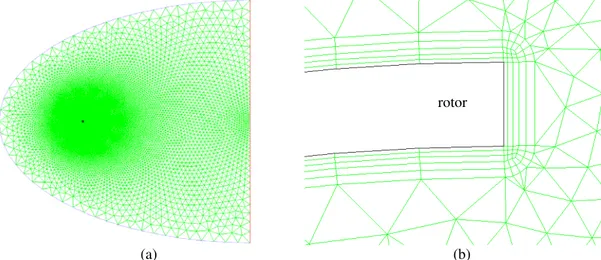
Figure 3(a) displays the mesh used in the simulation for the entire computational domain and the location of the Savonius rotor that appears as a black dot. To avoid the use of deforming dynamic mesh that is computationally more expensive owing to the mesh regeneration at each time step, a much simpler sliding mesh technique was used. For that purpose, a circle enclosing the rotor was created as the outer boundary of the sliding mesh, and the diameter of the circle is 2D (see Fig. 5 for the circle). This circle is a computational interface that is not a physical boundary. The black dot in Figure 3(a) is the circle and rotor, which have the size of 2D. The mesh surrounding the rotor inside the circle is allowed to rotate with the rotor when the fluid motion creates rotor rotation, whereas the other part of mesh outside the circle is stationary. In fact, there are two circles along the interface, one for the rotating inner mesh and the other belonging to the stationary mesh. The outer boundary of the computational domain is a semi-ellipse that is 300D wide in both the horizontal and the vertical directions. Although such a large computational domain is not necessary in producing reasonably accurate results, the outer boundaries were positioned very far away from the rotor so that the result is completely free from the influence of the outer boundary location. Since the flow is incompressible and two-dimensional without any three-two-dimensional relieving effect, it was observed in the numerical experiments that the air flow somewhat far away from the rotor is significantly influenced by the rotor, at least during some parts of rotation.
Wind velocity in the horizontal direction, V∞, was specified along the elliptical boundary in Figure 3(a) with the free stream turbulence viscosity ratio of 10, the atmospheric pressure along the vertical boundary on the right, and the no-slip condition at the rotor surface. Figure 3(b) displays five layers of structured quadrilateral mesh elements along the surface of the rotor and the near-wall region, which are critically important to resolve the unsteady turbulent boundary layer on the rotating blade. The height of the first quadrilateral element on the rotor is 0.1 mm in the direction perpendicular to the rotor surface, and it is compared in Fig. 3(b) with the thickness of the rotor blade equal to 2 mm. Unstructured triangular mesh elements were used away from the rotor surface due to their simplicity in creation.
Spalart-Allmaras model was adopted for turbulence modeling, the first-order implicit scheme for time advancement, and the second-order upwind scheme for the discretization of momentum and modified turbulent viscosity. The present analysis assumes turbulent flows although the flow may be partially laminar along the rotor blade surface during portions of rotations, at least under some of the conditions used in the simulations. To ensure the accuracy in time, PISO (Pressure-Implicit with Splitting of Operators) algorithm was chosen for pressure-velocity coupling scheme in the pressure-based solution method of ANSYS FLUENT. The unsteady
rotor
(a) (b)
simulations were performed by parallel processing, some of which used Beowulf Zeus cluster at the author’s institution (64-bit, 3.2 GHz, 4GB RAM).
3. Results and Discussion
A fixed time step of t = 10–4 sec was used in all the time-dependent simulations to ensure the accuracy. In convergence tests, the change in the results from t = 10–4 sec to t = 10–5 sec was negligibly small at the wind speed of 5 m/sec, which produced average rotor angular speed of 69.52 rad/sec (the actual time for one full rotation was 0.0896 sec) with the steady oscillation period in of 0.0448 sec (i.e., oscillation frequency of 140
rad/sec). Note that the steady oscillation of has two cycles for each rotation of the rotor, since the same motion is repeated every 180 degrees of rotor rotation.
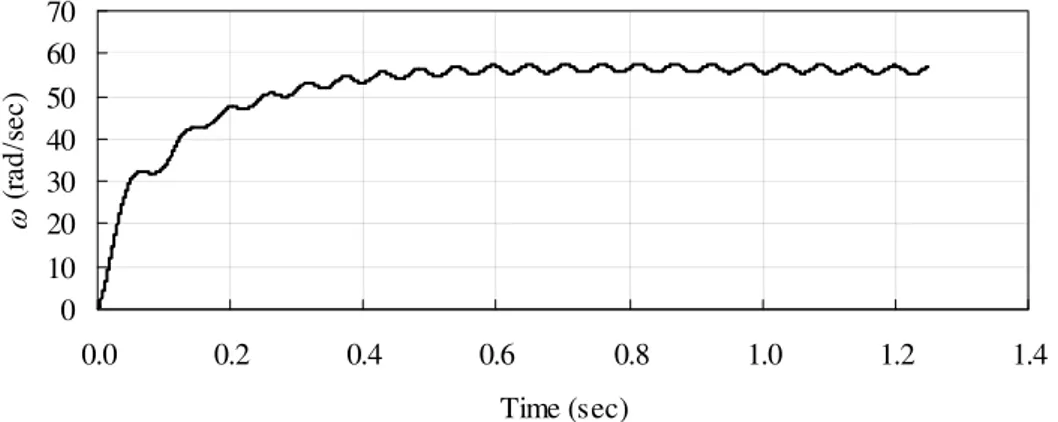
The Savonius rotor was held stationary under the wind of 4 m/sec until a steady flow was achieved, and then released at t = 0 marked in Figure 4, which clearly shows the transient behavior of the rotor, including the cyclic variation during the quasi-steady state when the angular speed varies periodically. The periodic positive angular speed indicates that the net moment acting on the rotor is negative during a portion of each rotation, i.e., Tr < Tg, < 0, and thus is decreasing; however, the sign change of causes to increase later in the same cycle. The average angular speed in the last rotation of the rotor presented in Figure 4 is calculated to be 56.1 rad/sec and the period of rotation is 0.111 sec, although it turns out that the angular speed is not yet fully converged to a steady oscillation.
Illustrated in Figure 5(a) is the contour plot of the static gage pressure in the vicinity of the rotor rotating in the counter-clockwise direction, presented at t = 1.2512 sec with the wind speed of 4 m/sec. The condition corresponds to the last point in the curve of Figure 4. As explained earlier in section 2, the circle is the sliding interface between the two fluid zones, which is a non-physical boundary used for purely computational purpose.
0 10 20 30 40 50 60 70
0.0 0.2 0.4 0.6 0.8 1.0 1.2 1.4
Time (sec)
(
rad
/s
ec)
Figure 4. Time-dependent angular velocity (V∞ = 4 m/sec and c2 = 0).
(a) (b)
The pressure values listed in the color map are in Pascal, and the atmospheric pressure away from the rotor was verified although not shown in the magnified view. The highest pressure is observed near the nose of a bucket moving in the direction opposing the main flow, whereas the concave surface on the other bucket facing the free stream wind has much lower pressure since the part moves in the direction of the main flow. Most part of the downstream side of the rotor has low pressure due to its orientation relative to the main flow. The instantaneous aerodynamic torque calculated with the distributed forces acting on the rotor surface turns out to be 0.0459 N·m (per meter), which is greater than the generator torque and thus produces a counter-clockwise net moment, even if the highest pressure point tends to create clockwise moment at the instant under discussion .
In Figure 5(b), the velocity vector field at the same instant as that of Figure 5(a) is illustrated with the color map legend presented in meters per second. To the left of the rotor, the flow is somewhat decelerated from the free stream wind, but the air speed is nearly doubled in the vicinity of the lower bucket moving in the direction of the main flow. Rotation of the rotor creates a circulating air motion around it, which in turn interacts with the free stream wind blowing from the left and produces a few regions with very small air velocity, one to the left of the upper bucket moving toward the free stream and another behind the same bucket. At two locations around the rotor center, small circulating regions are observed, which are associated with the nearly circular closed contours with low pressure in Figure 5(a). At the instant of time, the height of the first cells adjacent to the rotor surface yields the highest value of the inner-law variable, y+, slightly less than 2 observed only at two grid points, and the values of y+ are less than 1.6 at all the other grid points, producing the average of approximately 0.8. The inner-law variable is defined as y+ = yu*/, where y is the height of the first cell, is the fluid kinematic viscosity coefficient, and u* is the wall-friction velocity written as following, with w representing the
shear stress at the rotor wall:
w
u* (6)
Figure 6 shows the time-varying aerodynamic torque and mechanical power of the rotor during one full rotation at the wind speed of 4 m/sec, where the power is obtained by the product of the torque and angular speed at each instant of time. The results for the angle-dependent power of reference [5] showed a cyclic behavior similar to that obtained in the present work. Measurements of reference [6] also showed aerodynamic torque depending on the rotation angle, although both [5] and [6] assumed constant angular velocity in their theories. In Figure 6, the aerodynamic torque curve is nearly the same as the net torque curve due to the small magnitude of Tg at the operating values of . The angular speed increases for positive net torque and decreases
for negative net torque, and the instantaneous power of the rotor varies with the aerodynamic torque. Since the power in Figure 6 is negative during portions of cycle, it is possible to increase the cycle-averaged output power of the system by adopting a proper control mechanism. In another simulation, a constant angular velocity equal to 56.1 rad/sec (the cycle-averaged value of Figure 6) was enforced as in the conventional method, and the simulation was conducted until steady oscillation was obtained in the aerodynamic torque. The results of constant angular velocity simulation produced aerodynamic torque and mechanical power very similar to and slightly different from those of Figure 6, which produced nearly the same averaged power during the rotation. The very small difference in the two different simulations is attributed to the small percentage variation of angular velocity during the rotation, exhibited in Figure 6 and 4. Notice that the time variation of angular velocity depends on the magnitude of mass moment of inertia as shown in Eq. (1).
-10 -5 0 5 10 15 20
1.14 1.17 1.19 1.22 1.24
T ime (sec)
Figure 6. Time-dependent torque and power of the rotor during one rotation (V∞ = 4 m/sec and c2 = 0).
*0.3 (rad/sec)
Rotor Power (W)
Three methods were considered to calculate the average power after the rotor angular velocity reached steady oscillations; (i) the product of averaged Tr and averaged , (ii) the average of instantaneous power, i.e.,
the average of Tr·, (iii) the product of averaged and Tg evaluated at the averaged . All three methods
showed a good agreement with each other with negligibly small round-off error once the angular speed and the aerodynamic torque reached the steady oscillation. The third method is the most convenient in the present analysis producing time-varying properties with a specific generator, and it calculates the electric power output from the generator rotating at the average angular velocity of the Savonius rotor. During the rotation, Tr varies
periodically as and its average is equal to Tg evaluated at the averaged , once the quasi-steady state is
established.
Figure 7 shows a power-curve comparison between a theory, a few experiments, and the present computations. The black solid curve represents a two-dimensional theory of reference [6] based on experimental observations, but it neglects fluid friction, blade thickness, flow separation, turbulence, and time-dependence of angular velocity. Experimental data from various sources are shown by open symbols. The experimental data were adopted from reference [6], which also describes the sources of the data. The results of the present work, obtained from two-dimensional flow simulations, are indicated by red solid squares, and they exhibit a good agreement with the theory and some of the experiments. In Figure 7, the horizontal axis is the tip speed ratio, = (D/2)/V∞, and the vertical axis is the normalized power coefficient (Cp) defined as
H D V P
Cp 2
) 2 / 1 ( 17 . 0
1
(7)
where the factor 0.17 normalizes the power coefficient, P is the dimensional rotor power, is the air density, V∞ is the free stream wind speed, D is the rotor diameter, and H is the rotor height. As demonstrated by reference [8], it is necessary to vary both the wind speed and the rotor angular speed in order to produce a non-dimensional power curve and to identify the optimum operating condition. In the present analysis, a few different wind speeds were used, and the angular velocity at steady oscillation was varied by changing the generator heftiness through the value of c2. The data to cover the entire power curve were not obtained since it becomes more difficult for the small Savonius wind turbine to reach the steady oscillation at low wind speeds and additionally the present results are very sensitive to the value of c2 as the wind speed decreases. Due to these reasons, the present analysis show very sparse data for the left side of the power curve.
Reference [6] mentions that the experimental data have wide variation due to the differences in conditions, e.g., a small gap between the two buckets, but the theory shown by the black curve in Fig. 7 does not have any gap and thus has the same geometry as that of the present analysis. In addition, reference [6] states that much of experimental data are questionable due to wind tunnel blockage problems. Later, reference [9] performed thorough experiments regarding wind tunnel blockage of vertical-axis wind turbines. Note that the experimental
0 0.2 0.4 0.6 0.8 1 1.2
0 0.1 0.2 0.3 0.4 0.5 0.6
/ Cp
results in Fig. 7 have three-dimensional rotors, whereas the present results were obtained for a two-dimensional rotor without three-dimensional relieving effect.
The usual practice in wind turbine designs is to produce the power curve of turbine rotor valid for any generators and then determine the operating conditions for the generators considered. On the contrary, the approach demonstrated in the present analysis predicts the power curve by using specific generators, and then the operating points can be determined in the conventional way.
4. Conclusion
Unsteady rotations of a simple two-dimensional Savonius rotor were successfully simulated in order to demonstrate the capability of predicting the time-dependent properties of the rotor connected to a specific type of generator. The methodology is distinguished from the conventional ones, in that it can predict the actual angular velocity of the rotor during the rotation, instead of fixing the angular velocity to an arbitrary value by assuming an arbitrary generator. The principle and logic used in the present analysis can be conveniently applied to any type of rotating rigid turbines and also can be extended for non-rigid turbines. Thus the method can serve as an essential tool in the investigation of the transient behaviors of wind, water, or gas/steam turbines undergoing unsteady operation, and it is especially useful for, but not limited to, vertical axis wind turbines such as Darrieus and Savonius type turbines.
In the numerical experiments undertaken, it was possible not only to estimate the time-varying output powers in transient operations, but also to predict whether the turbine would rotate or not under certain conditions. The angular velocity, aerodynamic torque, and power of the rotor were all obtained in terms of time at various conditions, and the cycle-averaged powers at cyclically steady operations show a very good agreement with a theory and some experiments. It is also noticed that the current method can be extended to simulate multiple rotors that rotate simultaneously in a flow field.
Acknowledgments
Thanks are expressed to Dr. Jianhua Liu in Electrical Engineering Department at the author’s institution for helpful discussions on electric generators and associated electric power. The author would like to thank Mr. Aditya Gupte, a former graduate student at the author’s institution, for sharing his experience and motivating the author to put the long-delayed idea into practice. Additionally, the author is grateful for the computational resources provided by Aerospace Engineering Department of his institution.
References
[1] Duque, E. P. N.; van Dam, C. P.; Hughes, S. C. (1999): Navier-Stokes Simulations of the NREL Combined Experiment Phase II Rotor, AIAA-99-0037
[2] Sørensen, N. N.; Michelsen, J. A.; Schreck, S. (2002): Navier-Stokes Predictions of the NREL Phase VI Rotor in the NASA Ames 80-by-120 Wind Tunnel, AIAA-2002-31.
[3] Tongchitpakdee, C.; Benjanirat, S.; Sankar, L. N. (2005): Numerical Simulation of the Aerodynamics of Horizontal Axis Wind Turbines under Yawed Flow Conditions, J. Sol. Energy Eng., Vol. 127, Issue 4, pp. 464-474.
[4] Monteiro, J. M. M.; Páscoa, J. C.; Brójo, F. M R. P. (2009): Simulation of the Aerodynamic Behaviour of a Micro Wind Turbine, International Conference on Renewable Energies and Power Quality.
[5] Pope, K. (2009): Performance Assessment of Transient Behaviour of Small Wind Turbines, Master’s Thesis, University of Ontario Institute of Technology.
[6] Paraschivoiu, I. (2002). Wind Turbine Design with Emphasis on Darrieus Concept, Polytechnic International Press. [7] Nelson, V. (2009). Wind Energy: Renewable Energy and the Environment, CRC Press, Boca Raton.
[8] Mathew, S. (2006). Wind Energy: Fundamentals Resource Analysis and Economics, Springer.