www.ocean-sci.net/7/733/2011/ doi:10.5194/os-7-733-2011
© Author(s) 2011. CC Attribution 3.0 License.
Ocean Science
A computational method for determining XBT depths
J. Stark1, J. Gorman1, M. Hennessey1, F. Reseghetti2, J. Willis3, J. Lyman4, J. Abraham1, and M. Borghini5 1University of St. Thomas, School of Engineering, St. Paul, MN 55105-1079, USA
2ENEA, UTMAR-OSS, Forte S. Teresa, 19032 Pozzuolo di Lerici, Italy
3Jet Propulsion Laboratory, California Institute of Technology, Pasadena, CA 91109, USA 4Pacific Marine Environmental Laboratory/NOAA, Seattle, WA, 98115-6349, USA 5CNR-ISMAR, Forte S. Teresa, 19032 Pozzuolo di Lerici, Italy
Received: 13 June 2011 – Published in Ocean Sci. Discuss.: 2 August 2011
Revised: 17 October 2011 – Accepted: 27 October 2011 – Published: 8 November 2011
Abstract.A new technique for determining the depth of ex-pendable bathythermographs (XBTs) is developed. This new method uses a forward-stepping calculation which incorpo-rates all of the forces on the XBT devices during their de-scent. Of particular note are drag forces which are calculated using a new drag coefficient expression. That expression, obtained entirely from computational fluid dynamic model-ing, accounts for local variations in the ocean environment. Consequently, the method allows for accurate determination of depths for any local temperature environment. The re-sults, which are entirely based on numerical simulation, are compared with the experiments of LM Sippican T-5 XBT probes. It is found that the calculated depths differ by less than 3 % from depth estimates using the standard fall-rate equation (FRE). Furthermore, the differences decrease with depth. The computational model allows an investigation of the fluid flow patterns along the outer surface of the probe as well as in the interior channel. The simulations take account of complex flow phenomena such as laminar-turbulent tran-sition and flow separation.
1 Introduction
Accurate determination of the long-term trends in ocean heat content is essential for estimations of the impact of global warming on the planet. The ocean represents a significant reservoir and reacts slowly to changes in the Earth’s energy balance. The lag in ocean-thermal response and the very
Correspondence to:J. Abraham ([email protected])
large heat capacity of the ocean waters results in a significant portion of heat being absorbed there and is therefore critical for accurate prediction of future climate change.
That work also showed that uncertainties in the initial probe velocity overwhelm the impact of acceleration uncertainty. These findings demonstrate the difficulty in true comparison of XBT devices.
Currently, multiple classes of XBT probes are manufac-tured but the most common are referred to as T4/T6/T7/DB class and the T5 class. There are slight geometric differ-ences between the classes of XBT devices and therefore, it is expected that there are slightly different fall characteristics. Additionally, the devices are manufactured by two different companies (LM Sippican and TSK) and the manufacturing processes since the 1960s could have introduced small varia-tions in the geometry of the probes. Finally, alteravaria-tions made to the devices in subsequent generations have led to varia-tions in behavior so that year-to-year consistency is not guar-anteed (Wijffels et al., 2008; Gouretski and Reseghetti, 2010; Johnson, 2010; Kizu et al., 2011; DiNezio and Goni, 2010; Reseghetti, 2010).
With respect to the fall rate equations (FRE) originally supplied by LM Sippican, the inventor of the XBT probes, several works have tried to provide improvements over the manufacturer recommendations for the various XBT mod-els. Most of them concern the T4/T6/T7/DB class and are summarized by Hanawa et al. (1995), whose FRE has been considered the standard FRE for the T4/T6/T7/DB class from both the manufacturers. On the other hand, only few reports analyzed the T5 class (Boyd and Linzell, 1993; and Kizu et al., 2005a). Nevertheless, it has been argued that these FRE models cannot be universally applied around the differ-ent ocean waters with consistdiffer-ent accuracy. Specifically, there are experimental indications that the probe fall rate depends on the local water temperature (Hanawa et al., 1995; Green, 1984; Thadathil et al., 2002; Kizu et al., 2005b). Since the current FREs originated in experiments performed in tropi-cal or subtropitropi-cal waters, their application to polar regions or to water columns with temperatures differing from tropic regions may not be appropriate. Furthermore, use of the stan-dard FREs outside their range of applicability has a signifi-cant impact on ocean heat content estimation (Gouretski and Reseghetti, 2010).
It is believed that the dependency of FRE models on local conditions is a critical limitation to their accuracy, particu-larly when they are to be applied in different environments. Consequently, a new approach is proposed which calculates the fall rate of XBT devices for any local conditions. This method takes advantage of local temperature measured by the XBT itself to auto-correct for biases in the FRE. This new method requires very accurate determinations of the drag co-efficient and its variation with Reynolds number. The calcu-lation of the drag coefficient will be performed with greater fidelity than the earlier estimates of drag (Green, 1984; Hal-lock and Teague, 1992). While those earlier efforts were seminal and pioneering, the research was limited by the abil-ity to accurately determine the drag coefficient.
Advances in computational modeling now allow the
afore-mentioned limitation to be overcome. Numerical analysis of the fluid dynamics can account for details in physical geome-try of the probe and complex mechanics in the fluid. Included here is the accounting of laminar-turbulent transition of the fluid boundary layer against the probe body.
Here, a mathematical model will be presented to determine the depth of an XBT T-5 probe during a recent experimental launch. The method is not fully predictive because it relies upon local temperature measurements made by the probe for the determination of depth. The results will make use of pre-viously calculated drag coefficients that were obtained using numerical simulation. Probe depth will be determined with a forward-stepping time integration.
2 Numerical model
The numerical model has two important components. The first is the depth-calculation algorithm, second are the results for the Reynolds-dependent drag coefficient. Both portions of the numerical procedure will now be presented.
2.1 Depth calculations
The depth of the probe is based on a force-balance which is shown in Eq. (1). It can be seen that the net force on the probe is a combination of buoyancy and drag forces. Their differ-ence is equal to the change in probe momentum. Changes in momentum arise from velocity variations as well as varia-tions in the mass as the transmitting wire unspools.
Fnet=Fbuoy−Fdrag=
d mpV dt =mp
dV dt +V
dmp
dt (1)
The termmprepresents the instantaneous mass of the probe anddmp/dtis the rate at which that mass decreases from wire loss. The buoyant force is equal to the difference between the probe weight and the weight of displaced water,mwg; as is common in the literature so that
Fbuoy= mp−mwg (2)
whereas the drag force is found from the classic definition of the drag coefficient to be
Fdrag=Cd 1 2ρV
2A (3)
which can be rearranged to give
Cd= 2Fdrag
ρV2A (4)
Eqs. (1)–(4) are combined and the chain rule of differentia-tion is applied, there is obtained
mp−mwg−Cd 1 2ρV
2A=m p
dV dx
dx dt +V
dmp dx
dx dt
=mpV dV
dx +V 2dmp
dx (5)
which can be rearranged to give dV
dx =
mp−mwg−Cd12ρV2A−V2 dmp
dx mpV
(6) wherex is in the vertical direction. This model accounts for variations in the XBT velocity with depth but it does not account for unsteadiness in the ocean currents, that is, it as-sumes a quiescent water body.
While Eq. (6) is a viable representation of the variation in probe velocity, it is not solvable for velocity. Consequently, a finite-difference discretization is applied to Eq. (6) to give, after rearrangement
Vnew=V+1t
mp
mp−mwg−Cd 1 2ρV
2A−V2dmp dx
(7) whereVnewis the velocity at a future time step. All terms on the right-hand side of Eq. (7) are evaluated at a current time so that this numerical model marches forward in time steps of 0.1 s. It was found that the time steps were sufficiently small to ensure the results were independent of time step. Provided that the initial conditions of the launch (initial velocity and mass) are known, this equation can be evaluated. It must be emphasized that the use of Eq. (7) obviates the need for a tra-ditional FRE which relates depth to fall time. Equation (7) will, when accompanied with an expression for the drag coef-ficient, determine the depth of an XBT for any local environ-ment. It is also important to notice that the present method is able to account for differences in probe initial mass, the drop height, local water temperatures, and the linear-mass density of the wire.
2.2 Determination of the drag coefficient
Notably, the drag coefficient on the right-hand side of Eq. (7) must be known at each time step in order to proceed with the numerical integration. It is impossible to determine drag co-efficients analytically on blunt objects which cause flow sep-aration. Either experimental or computational investigations are required. Computational investigations offer a signifi-cant advantage over experimentation because of the ability to carefully control operating parameters and to determine drag coefficients for a wide variety of operating conditions. Typ-ically, drag coefficients are found to be single-valued func-tions of the Reynolds number, particularly when pressure forces dominate over frictional forces. Since the Reynolds number is, itself, a function of the local temperature, veloc-ity, and viscosity of the fluid, it follows that
Cd=function(Re)=function(T ,V ,µ) (8)
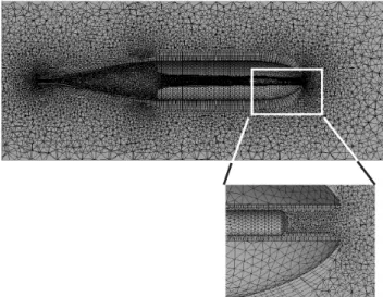
Fig. 1 – Image of the computational mesh with a close up view of elements near the probe nose.
Fig. 1. Image of the computational mesh with a close up view of elements near the probe nose.
With Eq. (8) available, the integration expressed in Eq. (7) can be completed.
2.3 The computational model
The first step in the determination of the drag coefficient is the discretization of the fluid region surrounding the probe. That discretization can be seen in Fig. 1. It may be noted that no fins are visible on the probe in Fig. 1 because the slice plane was selected to show elements on the main body of the probe. The simulations were fully three-dimensional and included all fins. This figure shows a bisected view of the probe and the mesh which spans the fluid domain. The mesh deployment was based on the knowledge of important pro-cesses which occur in the boundary layer. These boundary-layer processes govern the development of shear stress and pressure drag. It is essential for the elements to be fine within the boundary layer and aligned with the flow so that pro-cesses such as laminar-to-turbulent transition and boundary layer growth can be determined. It can be seen from Fig. 1 that the computational model extends around the exterior of the probe but also includes the flow that passes through the center channel of the device.
The governing equations include mass conservation, mo-mentum conservation, turbulence, and two transport equa-tions which govern the laminar-to-turbulent transition pro-cess. Each equation is solved at every computational element within the solution domain. This computational method, of-ten termed thefinite-volume method, is well established with a history of accurate fluid simulations.
The first equation in the set, conservation of mass, is ex-pressed in tensor notation as
∂ui ∂xi
The termui is the local velocity in thei-th direction. The next set contains three individual equations which represent conservation of momentum in the three coordinate direc-tions. Mathematically, it appears as
∂ ρuj
∂t +ρ
ui
∂uj ∂xi
= −∂p
∂xj
+ ∂
∂xi
(µ+µturb) ∂uj ∂xi
j=1,2,3 (10) Here, ρ is the local fluid density, p, is the pressure, µ is the molecular viscosity of the fluid, and the termµturbis the turbulent viscosity which is related to local fluctuations in the fluid velocity associated with turbulent motion.
A critical step in a computational fluid simulation is the determination of the turbulent viscosity. A variety of meth-ods have been used to accomplish this step, following the pioneering work of Launder and Spalding (1974) and of Wilcox (1988, 1994). More recent developments have com-bined the best features of these works into a comprehensive turbulent solution algorithm. That new approach was first proposed by Menter (1994) and is often termed theShear Stress Transport Model (SST). The SST model has shown ex-cellent capabilities of predicting flow separation, wall shear, and pressure variations in boundaries of blunt objects, such as XBT probes.
The SST model makes use of two transport equations for the turbulent kinetic energyκ, and the specific rate of tur-bulent dissipation, ω(inverse time scale). Those transport equations are
∂ (ρκ)
∂t +
∂ (ρuiκ) ∂xi
=γ·Pκ−β1ρκω
+ ∂
∂xi
µ+µturb
σκ ∂κ ∂xi (11) and ∂ (ρω) ∂t +
∂ (ρuiω) ∂xi
=AρS2−β2ρω2
+ ∂
∂xi
µ+µturb
σω ∂ω
∂xi
+2(1−F1)ρ 1 σω2ω
∂κ ∂xi
∂ω ∂xi
(12) A full description of the SST model and the terms in Eqs. (11) and (12) are provided in (Menter, 1994). The term γvaries between zero and one, taking values near zero for re-gions that are predominantly laminar and values near one for regions that are predominantly turbulent. It is used to multi-ply the rate of turbulence production,Pκ so that turbulence production is reduced where laminar flow dominates.
The termsβ1,β2, andAare model constants that result from experimental validation of the code. The SST turbu-lence model combines the very popularκ-ε andκ-ω mod-els. It uses theκ-ωmodel near the wall because of its su-perior performance in handling boundary layers. The code smoothly switches to the κ-ε model outside the boundary layer because of its superiority in that region. The smooth
transition is accomplished by the use of the blending func-tionF1. Theσ terms are model constants for the respective transported variable. More information can be obtained in the cited references.
The solution of coupled Eqs. (11) and (12) yields the val-ues for the turbulent viscosity which is expressed as
µturb=
aρκ max(aω,SF2)
(13) Equation (13) is a limiting function that eliminates the over-prediction of the turbulent viscosity; many turbulent mod-els are susceptible to this so that limiting functions are com-monly employed in computational fluid dynamics. TheF2 term is a blending function which restricts Eq. (13) to the boundary layer.
The final stage in the numerical procedure is to predict the status of the flow (laminar, intermittent, or turbulent). Most flow situations involve fluid motion that is a combination of these three states. For instance, flow near the leading edge of the XBT nose is likely to be laminar whereas flow near the aft is likely to be turbulent. There is a transitional region between the laminar and turbulent zones where the flow is partly laminar and partly turbulent. This laminar-to-turbulent transition is known to affect drag significantly (Gorman et al., 2010).
The transitional model used here was developed by Menter et al. (2002, 2004a, b) and later used by the present authors in a series of studies that conclusively demonstrated its suit-ability for flows of this nature (Abraham et al., 2008, 2009, 2010; Abraham and Thomas, 2009; Thomas and Abraham, 2010; Minkowycz et al., 2009; Sparrow et al., 2009; Lovik et al., 2009).
The transitional model consists of transport equations for the turbulent intermittencyγ, and the turbulent adjunct func-tion5which was first introduced by Menter et al. (2002) and then classified in Abraham et al. (2008). Those models are expressed as
∂ (ργ )
∂t +
∂ (ρuiγ ) ∂xi
=Pγ ,1−Eγ ,1+Pγ ,2−Eγ ,2
+ ∂
∂xi
µ+µturb
σγ ∂γ ∂xi (14) and ∂ (ρ5) ∂t +
∂ (ρui5) ∂xi
=P5,t+ ∂ ∂xi
σ5,t(µ+µturb) ∂5 ∂xi
(15) The production and destruction terms, (P and E) are de-scribed in Eqs. (4)–(5), (13)–(14), and (18) in Menter et al. (2004a). The origination of5 is shown in Eq. (16) of that same article. The value ofσ5 is taken from Menter et al. (2004a, b) to be 10 whileσγ is 1.0.
Table 1.Listing of parameters used in simulations.
Case Velocity Kinematic Viscosity Reynolds
(m s−1) (cm2s−1) Number (106)
1 6 0.0095 2.141
2 6.5 0.0095 2.319
3 7 0.0095 2.497
4 6 0.0103 1.974
5 6.5 0.0103 2.139
6 7 0.0103 2.303
7 6 0.0136 1.495
8 6.5 0.0136 1.620
9 7 0.0136 1.744
10 6 0.0146 1.393
11 6.5 0.0146 1.509
12 7 0.0146 1.625
At the inlet, positioned 0.45 m upstream of the probe, a uni-form relative velocity was given. At the exit, which was lo-cated 0.64 m downstream from the probe, an average gauge pressure was applied with weak conditions on all transported variables. At the probe surface, standard no slip conditions were employed. At lateral boundary conditions, which were positioned at least 7.5 cm from the probe, free-slip conditions were used. The simulations used a total of 2 100 000 ele-ments and the results were found to be independent of mesh size. Mesh independence was based on an increase in the number of elements by approximately 50 %. It was found that despite the improved resolution, the variation between the drag coefficients was insignificant. All calculations were performed using ANSYS CFX V12.1 software. Numerous simulations were completed for a range of velocities and vis-cosity values. Table 1 lists the parameters for the individ-ual simulations. In these calculations, the water density was treated as constant and equal to 1025 kg m−3. The frontal area of the T5 probe was found to be 0.00206 m2 and the probe length is 0.342 m, as listed in Table 3. The character-istic length in the Reynolds number is taken to be the probe length. In these simulations, no account was made for rota-tion of the probe during its descent.
We underline that during its motion an XBT probe has a rotation at a rate ranging between 10 and 15 rev/s as stated by LM Sippican, and reaches this condition within 2–3 s af-ter the probe hits the sea surface. If other factors such as entry angle or water turbulence due to the ship motion are considered, it is evident that the probe motion in the initial 20–30 m thick layer may be different from the standard mo-tion as described by the FRE. Recent videos indicate that the XBT motion in near surface layer is not vertically aligned but with slow rotation and helicoidal trajectory, confirming indi-cations quoted in Seaver and Kuleshov (1982).Therefore, a satisfying description of XBT motion in such a region is not easy to simulate.
Fig. 2 – Velocity contours (a) at the leading edge of the probe and (b) in the aft region
Fig. 2. Velocity contours(a)at the leading edge of the probe and
(b)in the aft region.
Further studies will be performed in the near future to ac-count for the rotation and helical motion. It is not known how large the impact of rotation is on the value of the drag coefficient. Drag is caused by pressure forces and by friction between the fluid and the probe surface. It is possible that the impact of rotation will be to increase frictional drag but reduce pressure drag. Finally, the entirety of the probe was modeled, symmetry conditions were not employed.
3 Results and discussion
Results from the numerical simulations will be presented first in a qualitative manner with a focus on the flow patterns which occur along the body of the T5. Next, quantitative results of the drag coefficients will be provided. Finally, the drag coefficients will be used to estimate the depth of T5 when field data on temperature and fall-time are available. Figure 2 shows a set of velocity contour diagrams near the (a) leading edge of the probe and in the (b) rear of the probe. The results in this figure and the following figure are repre-sentative of the set of results obtained using the information in Table 1.
Notable and expected features are easily observed. First, there is a local slow-fluid zone at the forward cone of the probe, near the center channel inlet. Second, it can be seen that fluid passes through the center channel and complicated recirculation regions are seen within the cavity. Finally, a recirculation region is seen behind the probe with relatively low velocities.
Fig. 3. Velocity streamlines(a)near the probe inlet and(b)in the probe interior.
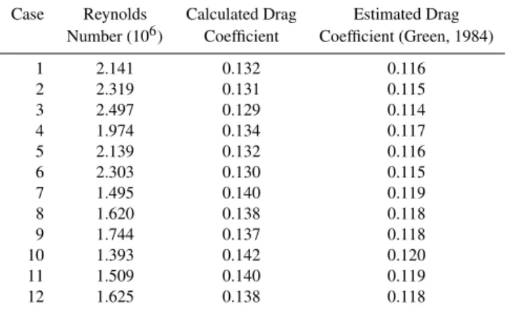
Table 2. Comparison of calculated drag coefficients with those from Green (1984).
Case Reynolds Calculated Drag Estimated Drag
Number (106) Coefficient Coefficient (Green, 1984)
1 2.141 0.132 0.116
2 2.319 0.131 0.115
3 2.497 0.129 0.114
4 1.974 0.134 0.117
5 2.139 0.132 0.116
6 2.303 0.130 0.115
7 1.495 0.140 0.119
8 1.620 0.138 0.118
9 1.744 0.137 0.118
10 1.393 0.142 0.120
11 1.509 0.140 0.119
12 1.625 0.138 0.118
The critical result which is required for the estimation of probe depth is the drag coefficient. In the present simula-tions, drag coefficient was found from Eq. (4) where the drag force was found from the simulations. The listing of results is shown in Table 2, along with a comparison to results which would be obtained with the estimation that is recommended in Green (1984). Graphical comparison of the present results with those of Green (1984) are shown in Fig. 4.
There are a number of features which are evident from the figure. First, the numerical simulations show a drag co-efficient that depends only on the Reynolds number. This finding is reassuring because it is expected from basic fluid-mechanic theory when pressure drag forces dominate over frictional drag. Second, it can be seen that the present results show values of the drag coefficient which consistently exceed those of Green (1984). In the figure, a fit of the presently
cal-Table 3.Parameter values used for fall calculations.
Parameter Value
Initial probe mass 0.98 (kg)
Mass of wire per unit length 0.000118 (kg m−1)
Probe length 0.342 (m)
Probe frontal area 0.00203 (m3)
Launch height 2.5 (m)
Initial probe velocity 7 (m s−1)
Initial probe displaced volume 0.000274 (m3)
Wire diameter 0.00762 (cm)
Density of surface water 1028 (kg m−3)
Fig. 4. Comparison of present drag coefficient results with those from Green (1984).
culated drag coefficient to Reynolds number is shown with the resulting expression
Cd=2.74×10⁻¹⁵·Re2−2.21×10⁻⁸·Re+0.1668 (16) The results of the present work also display a greater de-pendency of the drag coefficient on Reynolds number. It is relevant to identify a rational basis for the disagreement of the drag coefficients of the present work with those of Green (1984). Green’s results were taken from literature that presented drag values for streamlined bodies with con-trolled turbulence (Hoerner, 1965). That work provided only generalized values for various streamlined shapes. General-ized models are incapable of providing probe-specific drag results. Although the work of Hoerner (1965) and the in-corporation of drag into probe depth calculations were very advanced at the time, it was, admittedly, limited by the infor-mation that was available.
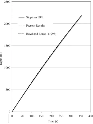
Fig. 5. Comparison of present depth results with values ob-tained from the manufacturer FRE and the FRE from Boyd and Linzell (1993).
were compared to numerical predictions. The parameters used in the simulations are listed in Table 3.
XBT T-5 probes manufactured by LM Sippican in 2002, 2003, 2007, and 2008 were launched during CTD casts from the CNR’s R/VURANIA, in Central and Western Mediter-ranean Sea. The recording system consisted always of a LM Sippican MK-21 USB and a notebook computer. The XBT sampling rate was 10 Hz, as great as the time con-stant of the XBT thermistor, having an instrumental sensitiv-ity of 0.01◦
C. The recording system was checked through a tester probe at two reference values (Tmin=12.75◦C,Tmax= 27.96◦C). The weights of deployed T-5 probes were within
the range 972.4–988.1 g, whereas the density of the copper wire varied from 0.118 to 0.121 g m−1. The height of the launching platform was always 2.5 m over the sea level, as high as the manufacturer suggests. Usually, the nose of the probes was thermalised in a bucket filled by seawater just before the drop.
Two independent tests of the new method will be pre-sented. The first test will be a comparison of the predicted depths from the new method with those which are obtained using the standard FRE. The second test will be a
compari-Fig. 6a.Percent deviation of present results from the manufacturer supplied FRE predictions.
Fig. 6b.Difference in depth calculations (new method – manufac-turer FRE).
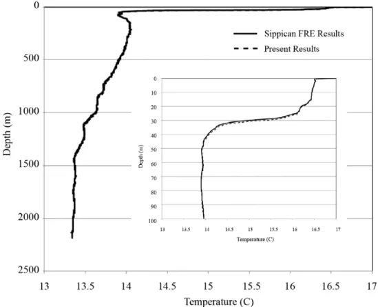
Fig. 7.Comparison of present depth-temperature results with current manufacturer FRE.
complemented by comparisons with the CTD devices, these two comparisons will provide quantitative information sup-porting the proposed method.
A comparison between the predicted depth using the cur-rent manufacturer supplied FRE and the present results is dis-played in Fig. 5. The level of agreement encourages the uti-lization of the present predictions which are based on numer-ical simulation. It can be seen that the present results slightly overestimate the depth of the probe compared to the man-ufacturer supplied FRE. This behavior can be explained by a number of reasons. First, the simulations were performed on a non-rotating probe. Furthermore, the comparisons are based on a single XBT drop. Deviations from one XBT drop to another may also give rise to some of the differences noted here. It is expected that when rotational motion is consid-ered, the results will be brought into even closer agreement. It is also expected that rotation will lessen the dependency of the drag coefficient on the Reynolds number. Also shown in Fig. 5 are the depth results using the Boyd and Linzell (1993) FRE. It can be seen the all three results are virtually indistin-guishable from each other.
Another useful comparison is shown in Fig. 6a and b, where the percentage deviation and the absolute depth de-viation (in meters) between the present results and those of the manufacturer supplied FRE are shown. It can be seen that the results differ by less than 3 % and the deviation decreases
with depth. For instance, at a depth of 1000 m, the differ-ence between the present method and the Sippican FRE is approximately 1.5 %, and decreases to about 0.1 % at depths of 2000 m. It is seen that the maximum difference of ap-proximately 15 m occurs at a depth of apap-proximately 1200 m. The shape of this curve gives insight about the relative fall rates. In the upper part of the ocean (less than 1200 m, the new method slightly over-predicts XBT depth whereas in the deeper regions, the new method under-predicts depths. Both the under-prediction and the over-prediction are slight, as represented by the small differences compared to the over-all depth measurements, and within the tolerance admitted by the manufacturer FRE (2 % or 5 m, whichever is greater). A further way to compare the present results with those using the manufacturer supplied FRE is to show the tem-perature/depth relationship. This information is provided in Fig. 7, where depths of the present method are compared with those from the Sippican FRE. It can be seen, at least on the scale shown in the figure, that the results are virtually indis-tinguishable from each other. An inset in the figure is used to provide greater resolution in the near-surface region.
Fig. 8. Comparison of averaged differences between the new method and CTD experiments with differences using the FRE ap-proach and CTD experiments.
profiler, calibrated before and after each cruise at NURC (NATO Undersea Research Centre, La Spezia – Italia). The CTD has a 24 Hz sampling rate, its nominal accuracy of 0.001◦C on temperature, and of 0.0003 Sm−1on conductiv-ity. Its time constants are 0.065 s for conductivity and tem-perature sensors (the nominal spatial resolution is 0.065 m), and 0.015 s for the pressure sensor (the spatial resolution is 0.015 m). The adopted lowering speed was 1.0 m s−1. CTD profiles were processed following standard SeaBird’s proce-dures (data conversion, alignment, cell thermal mass, filter-ing, derivation of physical values, bin average and splitting). In order to carry out such a comparison, all XBT profiles were interpolated to 1 m depth increments through a polyno-mial fit. Then, the temperature differences between the XBT profiles and the CTD measurements were calculated. The average temperature difference at each depth and the stan-dard deviation were calculated for both the versions of XBT profiles. The results are shown in Fig. 8.
Differences for all CTD/XBT temperature measurements were found for all coincident depths. It was discovered that the RMS values of the averaged FRE-CTD (0.068◦
C) and the new method-CTD (0.070◦
C) agreed to approximately 0.002◦
C.
A graphical display of a comparison between the present method and a collocated FRE experiment is shown in Fig. 9. This drop was performed on 8 October 2007. With the CTD drop made approximately 7 min prior to the XBT. In both figures, three sets of results are shown, the present method, the recommended FRE, and the results from the CTD device. The close agreement of the three sets of data serves to rein-force the method and indicate that the new method can be used to reproduce archival XBT data.
(a)
(b)
Fig. 9. Comparison of the present method with a collocated CTD experiment.
4 Concluding remarks
This work presents a novel treatment of calculating the depth of an XBT device during an oceanographic measure-ment. The method takes advantage of advanced computa-tional fluid dynamic software to calculate the drag coefficient with Reynolds number. Twelve separate calculations were performed for a non-rotating T5 device. It was found that the drag coefficient did not depend separately on the various operating parameters but rather depended solely on the value of the Reynolds number. This result concurs with basic fluid dynamic expectations.
(mass, size, etc.) or the parameters of the drop (height above water). The method takes advantage of the temperature mea-surements made by the probe during its descent. The temper-atures are utilized to determine instantaneous Reynolds num-bers and subsequent drag coefficients. This method avoids the reliance upon traditional fall rate equations. Finally, the computational method allows an evaluation of the flow pat-terns in the near vicinity of the probe and of the flow within the probe’s central channel.
The method was applied to a T5 experiment where it was found that the model agreed with CTD and the manufacturer supplied FRE. The agreement improved with depth.
The present work will be expanded to include the T4/T7/DB class of XBT devices. Additionally, inclusion of rotating motion will be made to assess its impact on drag.
Edited by: J. M. Huthnance
References
Abraham, J. and Thomas, A.: Induced Co-Flow and Laminar-to-Turbulent Transition with Synthetic Jets, Comput. Fluids, 38, 1011–1017, 2009.
Abraham, J., Tong, J., and Sparrow, E.: Breakdown of Laminar Pipe Flow into Transitional Intermittency and Subsequent Attainment of Fully Developed Intermittent or Turbulent Flow, Numer. Heat Tr.-B Fund., 54, 103–115, 2008.
Abraham, J., Sparrow, E., and Tong, J.: Heat Transfer in All Pipe Flow Regimes – Laminar, Transitional/Intermittent, and Turbu-lent, Int. J. Heat Mass Tran., 52, 557–563, 2009.
Abraham, J. P., Sparrow, E. M., Tong, J. C. K., and Bettenhausen, D. W.: Internal Flows which Transist from Turbulent Through Intermittent to Laminar, Int. J. Therm. Sci., 49, 256–263, 2010. Boyd, J. and Linzell, R. S.: The Temperature and Depth Accuracy
of Sippican T-5 XBTs, J. Atmos. Ocean. Tech., 10, 128–139, 1993.
Boyer, T., Gopalakrishna, V. V., Reseghetti, F., Naik, A., Suneel, V., Ravichandran, M., Mohammed Ali, N. P., Mohammed Rafeeq, M. M., and Chico, R. A.: Investigation of XBT and XCTD Biases in the Arabian Sea and the Bay of Bengal with Implications for Climate Studies, J. Atmos. Ocean. Tech., 28, 266–286, 2011. DiNezio, P. N. and Goni, G. J.: Identifying and Estimating Biases
Between XBT and Argo Observations Using Satellite Altimetry, J. Atms. Ocean. Tech., 27, 227–240, 2010.
Gorman, J. M., Sherrill, N. K., and Abraham, J. P.: Analysis of Drag-Reducing Techniques for Olympic Skeleton Helmets, AN-SYS Users Conference, Minneapolis, MN, 11 June 2010.
Gouretski, V. and Koltermann, K.: How Much is the
Ocean Really Warming, Geophys. Res. Lett., 34, L01610, doi:10.1029/2006GL027834, 2007.
Gouretski, V. and Reseghetti, F.: On Depth and Temperature Biases in Bathythermograph data: Development of a New Correction Scheme Based on Analysis of a Global Ocean Database, Deep-Sea Res. Pt. I, 57, 812–833, 2010.
Green, A.: Bulk Dynamics of the Expendable Bathythermograph, Deep-Sea Res., 31, 415–426, 1984.
Hallock, Z. and Teague, W.: The Fall Rate of the T-7 XBT, J. At-mos. Ocean Tech., 9, 470–483, 1992.
Hanawa, K. and Yoritaka, H.: Detection of Systematic Errors in XBT Data and Their Correction, J. Ocean. Soc. Japan, 43, 68– 76, 1987.
Hanawa, K., Rual, P., Bailey, R., Sy, A., and Szabados, M.: A New Depth-Time Equation for Sippican or TSK T-7; T-6; and T-4 Ex-pendable Bathythermographs (XBT), Deep-Sea Res., 42, 1423– 1451, 1995.
Heinmiller, R., Eddesmeyer, C., Taft, B., Olson, D., and Nikitin, O.: Systematic Errors in Expendable Bathythermograph (XBT) Profiles, Deep-Sea Res., 30, 1185–1197, 1983.
Hoerner, S.: Fluid-Dynamic Drag, Hoerner Dynamics, Bricktown, NJ, 1965.
Johnson, G.: Echo Sounder Evaluation of XBT Drop Rate Off the Coast of Florida, XBT Bias and Fall Rate Workshop, Hamburg, Germany, 25–27 August 2010.
Kizu, S., Itoh, S., and Watanabe, T.: Inter-manufacturer Difference and Temperature Dependency of the Fall-Rate of T-5 Expendable Bathythermograph, J. Oceanogr., 61, 905–912, 2005a.
Kizu, S., Yoritaka, H., and Hanawa, K.: A New Fall-Rate Equa-tion for T-5 Expendable Bathythermograph (XBT) by TSK, J. Oceanogr., 61, 115–121, 2005b.
Kizu, S., Sukigara, C., and Hanawa, K.: Comparison of the fall rate and structure of recent T-7 XBT manufactured by Sippican and TSK, Ocean Sci., 7, 231–244, doi:10.5194/os-7-231-2011, 2011. Launder, B. and Spalding, D.: Mathematical Modeling of
Turbu-lence, Comput. Method Appl. M., 3, 269–289, 1974.
Lovik, R. D., Abraham, J. P., Minkowycz, W. J., and Sparrow, E. M.: Laminarization and Turbulentization in a Pulsatile Pipe Flow, Numer. Heat. Tr. A-Appl., 56, 861–879, 2009.
Levitus, S., Anotonov, J., and Boyer, T.: Warming of
the World Oceans, Geophys. Res. Lett., 32, L12602,
doi:10.1029/2004GL021592, 2005.
Levitus, S., Antonov, J., Boyer, T., Locarnini, R., Garcia, H., and Mishonov, A.: Global Ocean Heat Content 1955–2008 in Light of Recently Revealed Instrumentation Problems, Geophys. Res. Lett., 36, L07608, doi:10.1029/2008GL037155, 2009.
Menter, F.: Two Equation Eddy-Viscosity Models for Engineering Applications, AIAA J., 32, 1598–1605, 1994.
Menter, F., Esch, T., and Kubacki, S.: Transition Modelling Based on Local Variables, 5th Int. Symposium on Engineering Turbu-lence Modeling and Measurements, Mallorca, Spain, 2002. Menter, F., Langtry, R., Likki, S., Suzen, Y., Huang, P., and Volker,
S.: A Correlation-Based Transition Model Using Local Vari-ables, Part I – Model Formulation, Proceedings of ASME Turbo Expo Power for Land, Sea, and Air, Vienna, Austria, 14–17 June 2004a.
Menter, F., Langtry, R., Likki, S., Suzen, Y., Huang, P., and Volker, S.: A Correlation-Based Transition Model Using Local Vari-ables, Part II – Test Cases and Industrial Applications, Proceed-ings of ASME Turbo Expo Power for Land, Sea, and Air, Vienna, Austria, 14–17 June 2004b.
Minkowycz, W. J., Abraham, J. P., and Sparrow, E. M.: Numerical Simulation of Laminar Breakdown and Subsequent Intermittent and Turbulent Flow in Parallel Plate Channels: Effects of Inlet Velocity Profile and Turbulence Intensity, Int. J. Heat Mass Tran., 52, 4040–4046, 2009.
Expendable Probes, J. Atmos. Ocean Tech., 8, 888–894, 1991. Reseghetti, F.: Performance of XBT Systems in Mediterranean Sea
(2003–2010), XBT Bias and Fall Rate Workshop, Hamburg, Ger-many, 25–27 August 2010.
Seaver, G. and Kuleshow, S.: Experimental and Analytical Error of the Expendable Baththermograph, J. Phys. Oceanogr., 12, 592– 600, 1982.
Sparrow, E. M., Abraham, J. P., and Minkowycz, W. J.: Flow Sepa-ration in a Diverging Conical Duct: Effect of Reynolds Number and Divergence Angle, Int. J. Heat Mass Tran., 52, 3079–3083, 2009.
Thadathil, P., Saran, A., Gopalakrishna, V., Vethamony, P., and Ar-aligidad, N.: XBT Fall Rate in Waters of Extreme Temperature: A Case Study in the Antarctic Ocean, J. Atmos. Ocean. Tech., 19, 391–395, 2002.
Thomas, A. and Abraham, J.: Sawtooth Vortex Generators for Un-derwater Propulsion, Open Mech. Eng., 4, 1–7, 2010.
Wijffels, S., Willis, J., Domingues, C., Barker, P., White, N., Gronell, A., Ridgeway, K., and Church, J.: Changing Expend-able Bathythermograph Fall Rates and Their Impact on Estimates of Thermosteric Sea Rise, J. Climate, 21, 5657–5672, 2008. Wilcox, D.: Reassessment of the Scale-Determining equations for
Advanced Turbulence Models, AIAA J., 26, 1299–1310, 1988. Wilcox, D.: Comparison of Two-Equation Turbulence Models for