www.atmos-chem-phys.org/acp/4/1323/
SRef-ID: 1680-7324/acp/2004-4-1323
Chemistry
and Physics
Longpath DOAS tomography on a motorway exhaust gas plume:
numerical studies and application to data from the BAB II campaign
T. Laepple, V. Knab, K.-U. Mettendorf, and I. Pundt
Institut f¨ur Umweltphysik, Ruprecht-Karls-Universit¨at Heidelberg, Heidelberg, Germany Received: 15 March 2004 – Published in Atmos. Chem. Phys. Discuss.: 7 May 2004 Revised: 28 July 2004 – Accepted: 9 August 2004 – Published: 23 August 2004
Abstract. This paper presents a procedure for performing and optimizing inversions for DOAS tomography and its ap-plication to measurement data. DOAS tomography is a new technique to determine 2- and 3-dimensional concentration fields of air pollutants or other trace gases by combining dif-ferential optical absorption spectroscopy (DOAS) with tomo-graphic inversion techniques. Due to the limited amount of measured data, the resulting concentration fields are sensitive to the inversion process. Therefore detailed error estimations are needed to determine the quality of the reconstruction. In this paper we compare different row acting methods for the inversion, present a procedure for optimizing the parameters of the reconstruction process and propose a way to estimate the error-fields by numerical studies. The procedure was ap-plied to data from the motorway emission campaign BAB II. Two dimensional NO2 cross sections at right angles to the motorway could be reconstructed qualitatively well at differ-ent meteorological situations. Additionally we presdiffer-ent error fields for the reconstructions which show the problems and skills of the used measurement setup. Numerical studies on an improved setup for future motorway campaigns show, that DOAS tomography is able to produce high quality concentra-tion maps.
1 Introduction
The measurement of trace gas concentration distributions in the atmosphere is an important tool for quantifying atmo-spheric emissions, chemistry and transport. It can contribute to the validation of chemical transport models (CTM), the improvement of emission inventories or for emission moni-toring (e.g. leakages in industrial installations).
Correspondence to:T. Laepple
1.1 Tomography for mapping trace gas distributions Two and three dimensional concentration distributions of trace gases can be obtained by combining path-integrating measurement techniques along a large number of light paths with tomographical inversion techniques. In comparison point sampling techniques can only give local details of the concentration maps and conclusions to larger scales may be falsified by small scale fluctuations. Tomographic line-integrating measurement techniques for trace gases were pro-posed by Wolfe (1980) and first indoor measurements were realized by Yost et al. (1994) using open-path Fourier in-frared absorption spectroscopy. Since then there have been improvements in speed and spatial resolution (e.g. Drescher et al., 1996; Fischer et al., 2001), but to our knowledge all ex-periments have been restricted to the laboratory environment so far.
1.2 DOAS tomography
experiments were carried out during the motorway campaign BAB II in 2001, which was organised by Fiedler et al. (2001). More details are given by Pundt et al. (2004), Knab (2003) and in Sect. 2.
In comparison to other tomographic applications like in medicine, DOAS-tomography has only a very limited num-ber (10–100) of well known light paths. Therefore the recon-struction technique is not time critical but attention has to be paid on the a-priori information added to the ill-posed prob-lem, implicitly by the algorithm or explicitly by the selected parameters. This requires extensive studies on the reliability of the reconstructed concentration fields. These studies are a main subject of this paper.
1.3 Overview over inversion techniques
Due to the limited amount of data in DOAS-tomography a discretization is needed which describes the concentration field by a finite number of parameters accepting losses in ac-curacy.
Drescher et al. (1996) proposed an inversion algo-rithm called smooth basis function minimization technique (SBFM) for the reconstruction of indoor trace gas measure-ments. The concentration field is parameterized nonlinearly as a sum of several Gaussians with some free parameters. A global optimization algorithm is used to determine the set of parameters fitting the measurement data best. While SBFM is reported to be suitable for indoor measurements examining the mixing of trace gas from located sources (Fischer et al., 2001), it could not be applied successfully in our case of a motorway exhaust plume. The plume shapes for the motor-way campaign estimated by a chemical transport model (D. B¨aumer, personal communication) could not be described by Gaussians with a number of parameters determinable by the measurement data. Sharp concentration slopes are appear-ing near emission sources, if the wind is blowappear-ing from one specific direction. This is not the case in indoor situations. Other parameterizations for the use at the motorway situation involved an unquantifiable amount of a priori information. One main problem is the difficulty to determine the quality of the reconstruction due to the nonlinearity of the inversion and the long computation time for the global optimization (in the order of hours for our problem size) which does not allow extensive numerical sensitivity studies.
The more common approach is to discretize the contin-uous concentration field by a linear combination of a finite number of basis functions. The advantage of this linear ap-proach is that the resulting discrete linear inversion problem is better to handle and does not require the knowledge of the algebraic form of the concentration field. (The nonlinear approach SBFM only works well if the concentration field can be described by superposition of few Gaussians). There-fore we use the linear approach. In the literature many meth-ods can be found to solve this linear inversion problem (e.g. Groetsch, 1993).
In environmental science a popular class of methods are iterative row-acting-methods (RAM). They were often used to deal with large size problems because they only act on the rows of a matrix and save memory space. Their simplic-ity and their good regularization and smoothing characteris-tics still makes them interesting and they are successfully ap-plied on tomographic problems (e.g. Kak and Slanley, 1988). In environmental sciences, Ziemann et al. (2001) use the si-multaneous iterative reconstruction technique (SIRT) a mem-ber of this algorithm class in acoustic tomography for deter-mining small scale land surface characteristics. Todd and Ramachandran (1994) use row acting methods for numeri-cal studies on FTIR-tomography. The disadvantage of these techniques is that the a priori information which is always needed to solve the ill-posed inversion problem is not added explicitly but is included in the nature of the algorithm, the first guess and the number of iterations.
There are inversion techniques which include the a pri-ori information explicitly. Application of a statistical ap-proach to atmospheric remote sensing can be found in Rodgers (2000). A constrained optimization method – where a smoothness function is used as quadratic constraint – is used successfully by Fehmers et al. (1998) in the field of the tomography of the ionosphere. If good a priori information is available these inversion techniques are useful to include such information. Further work has to be done to investigate these techniques and to investigate which a priori informa-tion can be integrated depending on the problem.
Due to their regular use in tomographic problems similar to our problem we decided to use row acting methods as a starting point for the new tomographic DOAS technique and the study described here. First we describe the discretiza-tion process and discuss different basis funcdiscretiza-tions and differ-ent row acting methods in Sect. 3. In contrast to other studies we try to investigate the complete characteristics of the cho-sen RAM’s by numerical studies in Sect. 5 and choose the best parameter set for our reconstruction. In Sect. 6 we apply this optimized algorithm on the motorway data.
Independent of the inversion technique it is important to quantify the quality of reconstructions. To our knowledge the absolute reconstruction error has not yet been estimated in to-mographic applications in atmospheric sciences. Drescher et al. (1997) compared reconstructed concentration fields with real point measurements. Todd and Ramachandran (1994) performed numerical experiments judging the reconstruction quality by some quality criteria, but only considering concen-tration fields constructed as sum of several randomly located Gaussians and ignoring the errors caused by the discretiza-tion. Price et al. (2001) mentioned errors due to measuring the light paths sequentially but did not quantify them.
1 6 0 m
8 2 5 m 7 0 5 m
D O A S 1 D O A S 2
x
y
z
1 6 0 m
8 2 5 m 7 0 5 m
( b ) ( a )
Fig. 1. DOAS tomography setups for the measurements of cross sections of vehicle exhaust gas plumes at right angles to the motorway. Setup(a)was used during the motorway campaign BAB II. Two DOAS telescopes were placed on opposite sides of the motorway. 4 retro-reflectors were mounted on two cranes in about 800 m distance. With the stepping technique 16 lightbeams were realized, 8 crossing and 8 going parallel to the carriageway. The enhanced setup(b), desribed in Sect. 6.7, consists of 4 telescopes and 9 retroreflectors. It is able to measure the cross sections with much better accuracy. For better clarity only the lightbeams of the telescopes on the left hand side are drawn in completely.
2 DOAS tomography measurements at a motorway
During the field campaign BAB II (Experimental determina-tion of emissions from motor vehicle traffic on motorways and comparison to calculated emissions) at the motorway A 656 in Germany , organized by the Institute for Meteo-rology and Climate Research (IMK) of the Forschungszen-trum Karlsruhe, first Longpath DOAS tomography measure-ments took place in April, May 2001. It was the first path-integrating tomographic 2-D outdoor measurement of trace gases. For details on the campaign please refer to Fiedler et al. (2001). The DOAS tomography measurements are de-scribed by Knab (2003) and Pundt et al. (2004).
A setup of 16 light paths was realized by using two con-ventional long-path DOAS systems and directing them suc-cessively towards eight retro-reflector arrays. The environ-mental conditions for the time period studied here were cho-sen deliberately: During that time there were both, a rela-tively continuous vehicle flux and undisturbed air crossing the motorway. Thus the situation was assumed to be homo-geneous in the direction of the carriageway and a concentra-tion cross secconcentra-tion at right angles to the motorway could be derived. The measurement setup is shown on the left part of Fig. 1.
The motorway induced turbulences and chemical transfor-mations at the measurement site which had been examined by Vogel et al. (2000) and B¨aumer (2003) with the mesoscale chemistry transport model system KAMM/ DRAIS. A NO2 concentration field generated with this model (D. B¨aumer, personal communication) was used for numerical experi-ments in this study and will, in the following, just be referred to as CTM BAB II plume (see Fig. 4a).
3 Tomography
The distribution of a trace gas in the atmosphere is usually described as a continuous concentration fieldc(r). Assum-ing the concentration field is known, a DOAS measurement along a light path LPi gives the data (slant column density)
di =
Z
LPi
drc(r). (1)
This is the forward model and is well known in our case. The unit of the data used here is ppb∗m which corresponds to the integrated concentration over the light path.
3.1 Discretization
A model is needed which describes the continuous concen-tration field with a finite number of parameters. We will call this a discrete state model. If there are m lightbeams resulting in m values of measurement datad1todm, they are
assembled to a data vectordand the n parameterss1tosn
de-scribing the state model concentration field in a state vector
s.
Data vectord=(d1, d2, ..., dm)t ∈D (2)
State vectors=(s1, s2, ..., sn)t ∈S (3)
The according vector spaces are called data (vector) space Dand state (vector) spaceS. A discrete state model can be realized by a family of n basis functions(bj)j∈{1..n}. Then
the model concentration fieldc(s,r)is a linear combination of the basis functionsbj(r)with the state vector components
sjas coefficients.
(a)
0 1 2 3 4 5 6
0 1 2 3 4
0 1 2 3 4 5 6
0 1 2 3 4
x-axis [✂✁ ]
co
n
ce
n
tr
at
io
n
[p
p
b
]
Box
basis function
(b)
0 1 2 3 4 5
0 1 2 3 4
0 1 2 3 4 5
0 1 2 3 4
x-axis [✂✁ ]
co
n
ce
n
tr
at
io
n
[p
p
b
]
Bilinear basis function
(c) original (d)5×4box model (e)5×4bil. int model
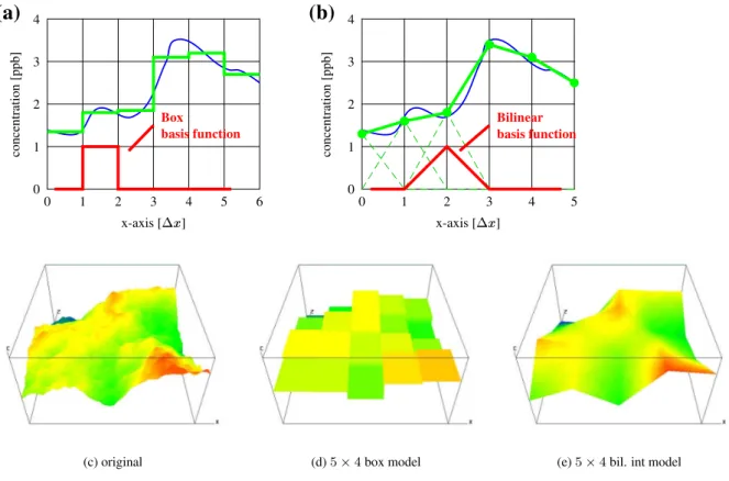
Fig. 2.Discretization models. The upper two subfigures show a 1-dimensional cross section of a concentration field. In the case of the box model(a)the real concentration field (blue) is approximated by a step function (green), which is constant within each box. For the bilinear interpolation model(b)the basis functions (red) are pyramid shaped. They have a peak of height one above the affiliated lattice point and reach zero at the neighboring lattice points. The resulting model function (green) is continuous and interpolates the values at the lattice points linearly. In subfigures(c),(d)and(e)the discrete modeling of a continuous 2-D function is visualized in color contour plots: A continuous concentration field (c), its best approximation with the 5×4 box model (d) and the 5×4 bilinear interpolation model (e).
The basis functions have to be linearly independent. Then for each continuous concentration fieldc(r) a unique state vector s exists that minimizes the misfit kc(r)−s·rk. In the following we assume the concentration to be invariant of the z-axis. This refers to the reconstruction of 2-dimensional cross sections of 3-dimensional trace gas fields. We investi-gate two kinds of discrete state models: the box model and the bilinear interpolation model.
3.1.1 Box model
For the box or pixel model (e.g. Kak and Slanley, 1988) the area of interest is divided into (usually rectangular) boxes. Each box corresponds to a basis function
bj(r)=
1 if r∈box j
0 else (5)
The model concentration fields thus are step functions which are constant within the boxes.
c(s,r)=
s1 if r in box 1 s2 if r in box 2 .
.
(6)
Here the state vector components are the model concentra-tions of the different boxes. Figure 2a shows a representation of a one-dimensional model field by such box functions. The concentration fieldc(r)is approximated best, if the height of the stepsj is the average concentration in the referring box:
sj= hc(r)iboxj.
3.1.2 Bilinear interpolation model
lattice pointrj=(xj,yj)refers to a bilinear basis functionbj:
bj =txj(x)tyj(y)
txj =
1−1x1 x−xj
if
x−xj
≤1x 0 else
tyj =analog,
(7)
where1x is the lattice width in x-direction. The basis func-tions are pyramid-shaped and have a peak of height 1 above the affiliated lattice point. The value of the modeled concen-tration field at the lattice points is given by the components of the state vector
c(s,rj)=sj for all lattice points rj. (8)
At the other points the model field is determined by bilin-ear interpolation of the values at the four neighboring lat-tice points. Figure 2b shows a representation of a one-dimensional model field by such bilinear basis functions.
Due to the continuity of the bilinear basis function they can describe a continuous concentration field better than the discontinuous box-basis functions. Therefore they are more appropriate in our case. In Fig. 2c and e, this is demonstrated by modeling a test concentration field using the two types of basis functions. The advantage of bilinear basis functions will also be confirmed in Sect. 5, where we compare the re-construction quality, using the box and the bilinear represen-tation in turns.
3.1.3 Resolution of the discretization
The state model has to describe the real concentration field as accurately as possible with a small number of basis functions n.
If the chosen resolution is not fine enough (too small di-mension of the state vector) the difference between the con-tinuous concentration field and the best discrete approxima-tion leads to errors due to the discretizaapproxima-tion, so-called “dis-cretization errors” in the reconstruction. If the resolution is too fine, the problem gets highly underdetermined and more a priori information is needed to solve the inversion problem. (A further discussion of these errors can be found in Sect. 4.) The best resolution is dependent on the information content of the measurements and the a-priori information available and will be determined in numerical studies in Sect. 5. 3.2 Discrete linear inverse problem
Approximating the real concentration field by the model field, the forward model (1) becomes d=Fs with forward matrix:
fij=
Z
LPi
drbj(r) (9)
In the case of the box model the entry fij of the forward
matrix corresponds to the length of light path i through box j. The problem of solving Eq. (9) for a given data vectordis
a discrete linear inverse problem.
This problem is in general ill-posed: If Eq. (9) is over- or mixed-determined no exact solution exists, but only an ap-proximate solution. If Eq. (9) is mixed- or under-determined the solution is not unique. If the condition number (e.g. the ratio of largest to smallest singular value of the matrix) of F is large, the solution is not stable, i.e. it is sensitive to small errors in the data.
The first problem can be overcome by using the approx-imate minimum misfit solution (least squares solution) as physical solution. The latter two problems can only be reme-died by adding additional a priori information, e.g. the infor-mation, that the concentration field either is positive allover or that it fulfills certain smoothness conditions. Often the minimum norm solution is demanded, but the a priori infor-mation to favor the state with the smallest norm is physi-cally not reasonable in our case. The approximate minimum norm minimum misfit solution is also known as generalized inverse, and can be calculated by singular value composition (SVD) (e.g. Groetsch, 1993).
To take the measurement error on the data into account, a weighting matrix W can be introduced which is the in-verse of the covariance matrix. If the noise on the data can be assumed to be uncorrelatedWis given by the elements
W ii=1/ε2i. The weighting is applied by the substitution:
∼
d←→W1/2d, ∼F←→W1/2F and ∼s←→s (10)
This is assumed to be already done in the following discus-sion.
3.3 Row acting methods
As mentioned in the introduction we use row acting meth-ods (RAM) in this study to solve the discrete linear inverse problem.
RAM are a class of iterative algorithms to solve linear sys-tems of equations – especially tomographic discrete linear in-verse problems. The common names of row acting methods like Algebraic Reconstruction Technique (ART) (Herman et al., 1973) combine an inversion technique (i.e. the technique for solving the system of Eq. 9) with a special discretization model (e.g. box, bilinear). As we want to use the algorithm independently from the discretization model, we use the sep-arate names “ClassicalName-like” to allow a better compari-son. (Our “ART-like” algorithm for example is the algorithm ART from the literature but independent of the discretization model.)
3.3.1 The ART-like method
0 1
✂✁
0 1
☎✄
✆✞✝
✆✠✟ ✆✠✡
initial guess
☛ ☞✍✌✏✎☛✒✑✓✔
☛ ✑✕✔
(a) sequential RAM (ART-like)
0 1 ✖✘✗
0 1
✖✚✙
✛✢✜
✛✤✣ ✛✤✥
✦★✧✩✪
✦ ✧✫✪ ✦ ✧✬✪
(b) simultaneous RAM (SIRT-like)
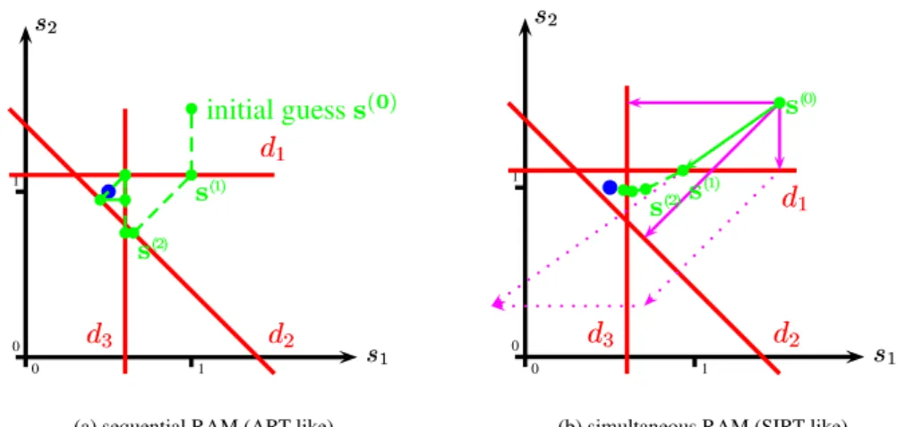
Fig. 3. Row acting methods (RAM) graphically. Each data point di refers to a hyperplane in state space (red lines). If an exact solution exists, it must lie on all these hyperplanes. Here the inverse problem is over-determined, and there is no exact solution (there is no intersection for all three hyperplanes). Starting point is the initial guess s(0). For the sequential RAM(a)the actual guess is iteratively projected onto one hyperplane after another. Because of the over-determination the iteration sequence (s(j ))(green) oscillates cyclically convergent in the neighborhood of the intersections of the hyperplanes. For the simultaneous RAM(b)the hypothetical changes due to projections onto all hyperplanes (pink vectors) are gathered first. Then their average (green vector) is added to the actual guess. Here the state vector sequence (s(j ))approaches the real state slowly but consequently.
in combination with box basis functions under the name al-gebraic reconstruction technique. It is based on the follow-ing idea: Each rowfi ·s=di of matrix Eq. (9) refers to one
data-point and fixes a (1) dimensional hyperplane in a n-dimensional state space, on which any existing solution must lie. This is shown graphically in Fig. 3a for one dimensional hyperplanes in a two dimensional space. If a solution exists, it is thus situated on the intersection of all n hyperplanes. The algorithm starts with an initial guesss(0). The solution is determined by iteratively projecting the actual guess onto a hyperplane and taking the result as new actual guess.
s(k+1)=s(k)+α( di
kfik
−s(k) fi kfik
) fi
kfik
, (11)
where i=(k mod m)+1.
Here k is the iteration number and i is the number of the hyperplane onto whichs(k)is projected in the actual iteration step. The damping parameterαis 1 for the basis algorithm. The optimal termination of the iteration can be determined in numerical experiments.
If a unique solution exists, the iteration sequence s(k)k∈N
converges to this solution. If the system of equations is un-derdetermined, s(k)
converges to the solution closest to the initial guess in the sense of the Euclidian vector norm. If the system of equations is mixed- or over-determined and the data vector is “noisy”, generally no solution exists. Then ART is cyclically convergent, i.e. after a lot of iteration the sequence s(k)
follows to a fixed closed trajectory of period m (e.g. Censor et al., 1983). In Fig. 3a this is the case be-cause this example is overdetermined and has no exact so-lution (three hyperplanes in a two dimensional state space).
In such cases a better convergence can be obtained by us-ing a dampus-ing parameterα decreasing from 1 to 0 in the course of the iteration. If the concentration field is zero at some locations, the convergence can be ameliorated, by set-ting negative values back to zero in each pass. For the mo-torway situation it would not have made any sense to use this technique . The row acting methods looked at here are im-plicitly smoothing the solution if the iteration is terminated prematurely. An optimum iteration number can be found by surveying the Iteration process by eye, by guessing roughly or as done in this study by numerical experiments.
3.3.2 The SIRT-like method
The combination of the simultaneous iterative projection method and a box discretization model is known as simul-taneous iterative reconstruction technique (SIRT) (Kak and Slanley, 1988).
This method differs from the sequential iterative projec-tion method, by the fact that the correcprojec-tion of a state due to the projection is not immediately applied. Instead, before making any changes to s all m equations are gone through calculating the hypothetical change due to the projection onto the hyperplane. At the end of one pass the average over all these hypothetical changes is taken and applied to the state vector:
s(k+1)=s(k)+ α
m Xm
i=1( di
kfik
−s(k)· fi kfik
) fi
kfik
guess (Van der Sluis and van der Vorst, 1987). This is shown in Fig. 3b which is based on the same equation system as in Fig. 3a but with the SIRT algorithm. The three hypothetical changes for the first step are explicitly plotted. For the other steps only the applied change to the state vector are shown. In contrast to Fig. 3a, the state vector converges to the minimum misfit solution.
3.3.3 The SART-like inversion method
Another modification is an algorithm known – in combina-tion with bilinear basis funccombina-tions – as simultaneous algebraic reconstruction projection method (SART)(Kak and Slanley, 1988).
The projections applied simultaneously as in the simul-taneous iterative projection method, but the weights of the corrections are different.
s(kj+1)=s(k)j +Pm1
i=1fij m
X
i=1
(di−s(k)·fi)fij
Pn
α=1fiα
(13)
Here the iteration sequence converges to a minimizer of a weighted least square functional from any initial guess (Jiang and Wang, 2001). The convergence is faster than that of the SIRT-like inversion method. In DOAS-tomography applica-tions (state vector size 10–100) the computation time for the row acting methods is about 1000–10 000 iterations per sec-ond on a 1 GHZ Pentium processor. Therefore the conver-gence speed is not important for our applications.
4 Error estimation
The reconstruction error field 1c(r) is the difference be-tween the concentration field reconstructed by a DOAS-tomography measurementcrec(r)and the real concentration
fieldcreal(r).
1c(r)=creal(r)−crec(r) (14)
For simplicity we will also call continuous test-fieldscreal(r)
which are used in numerical studies.
In this section we describe the sources of the reconstruc-tion error and a way to estimate them. The practical pro-cedures for optimizing the reconstruction process with re-spect to a low reconstruction error and for estimating the er-ror for the motorway campaign are presented in the referring Sects. 5 and 6.
4.1 Sources of the reconstruction error The reconstruction error has four causes:
1. the measurement error,
2. the discretization error in the data, 3. the discretization error in the state,
4. the inversion error.
For a better understanding we introduce the following oper-ator notation:
– D Discretization operator; maps a concentration field c(r)to the best approximation state vectors=Dc(r).
– D†Continuization’ operator; leads from the state vector s to the affiliated concentration fieldc(s,r)=D†s.
– FForward operator; forward models data from the dis-crete state vectord=Fs(see Eq. 9) .
– G Continuous forward operator; forward models data
from a continuous concentration field d=Gc(r) (see Eq. 1).
– F†Inversion Operator; describes the application of the inversion method to the datas=F†d.
The “continuization” operatorD†is a pseudo-inverse to the discretization operator D. The inversion operator F† is pseudo-inverse to the discrete forward modeling operatorF. In this notation the reconstruction and the simulation of a measurement and reconstruction are:
Reconstruction crec(r)=D†F†d (15)
Simulation crec(r)=D†F†Gc(r) (16)
The measurement error1dmeasis the difference between the
measured data and the data that would be obtained from an ideal experiment (i.e. data forward modeled from the real, continuous field). 1dmeasconsists of the error in the
indi-vidual measurement devices and the so called stepping er-ror, which occurs if the different light paths are not measured simultaneously. It is propagated through the inversion the same way as the data (because of the linearity of the two op-erators) yielding the propagated measurement error: 1cmeas(r)=D†F†1dmeas (17)
The discretization leads to errors in two ways: Firstly, an arbitrary continuous concentration field generally cannot be exactly approximated by the discretized field:D†D6=1.
Secondly, the forward modeling of measurement data from the discretized field differs from the data obtained from the real, continuous field:F D6=G.
If the inverse problem (9) does not have a unique solu-tion, i.e. because it is ill-posed, a priori information has to be employed to select a solution. The inversion error arises, because normally the a priori information is not completely correct.F†F6=1.
We get the sum of discretization errors and the inversion error in the concentration as
which corresponds to simulating a perfect measurement on a concentration field, reconstructing the field and comparing it to the original concentration field.
If all operators are linear – as it is the case for linear dis-cretization models and row acting methods (each projection step is linear and thus also the whole inversion), then the total reconstruction error is the sum of Eqs. (17) and (18): 1c(r)=1cmeas(r)+1cdi(r) (19)
Therefore the two parts can be treated separately which en-hances the computational speed of the error estimation and the knowledge about the error causes.
Usually the resolution matrixR=F†Fis introduced to vestigate the reconstruction quality. Using this matrix the in-version error can be determined as(1−R)srealneglecting the
discretization error. As we work with a moderate resolution, this disregarding is not acceptable in our case.
4.2 Estimation of the error fields
For the error estimation the error fields 1cmeas(r) and
1cdi(r)are considered as random functions and the aim is to
determine their random distribution (for simplicity, we use the same notation for the random function and it’s realiza-tion). In order to get the total reconstruction error1c(r)we have to convolute the two random distributions at the end.
The measurement error1dmeas is assumed to be a
Gaus-sian distributed random vector of mean zero. This means the propagated measurement error1cmeas(r)is also
Gaus-sian distributed and of mean zero. Assumedcovdmeasis the
covariance of the1dmeas and the continuous fields are
dis-cretized on a finite grid, then the covariance of the propagated measurement error is
covcmeas=(D†F†)(covdmeas)(D†F†)†. (20) The operatorD†F†can be determined by applying the inver-sion method on the m data basis vectors.
The discretization and inversion error1cdi(r)depends on
the shape of the field to be reconstructed. Consequently, a priori information is needed for determining1cdi(r).
With-out any a priori information on the concentration field, the re-construction error would be infinitely high. Imagine a DOAS tomography setup and a concentration field with a very steep and high peak in the gap between some light paths. Such peak is not detectable with the given setup. Only with infor-mation about smoothness such a field can be excluded. The concentration field to be reconstructed is a random function creal(r)and the prior information is represented by its
bility distribution. Applying Eq. (18) on it leads to the proba-bility distribution of the derived random function1cdi(r). In
practice the probability distribution ofcreal(r)was realized
by generating a set of test fields(ck(r))k∈N all of which are
assumed to have the same probability. Applying Eq. (18) to all of these test fields produces a set of reconstruction error fields(1cdik(r))k∈Nwhich can be evaluated statistically.
4.3 Reconstruction quality criteria
In simulations and validation experiments the reconstructed concentration field can be compared with a “real” field. Quality criteria are needed, which summarize the overall re-construction quality in a single figure. They can be used in numerical simulations to determine optimum reconstruction techniques and parameters. Apart from the criterion “near-ness”, which has been used in former studies (e.g. Todd and Ramachandran, 1994), we suggest here two further criteria, the “normalized maximum difference” and the “normalized average difference”. The choice of the criterion depends on the further use of the reconstruction result. All of the pro-posed criteria are calculated from the reconstruction error 1c(r)=creal(r)−crec(r)and the “real” fieldcreal(r).
4.3.1 Nearness
The quality criterion nearness is a normalized 2-norm (Eu-clidian norm) of the reconstruction error:
Nearness= N1 k1ck2
= N1 q
R dr2(c
rec(r)−creal(r))2
where N = q
R dr2(c
real(r)−creal(r))
2 .
(21)
Normalization makes the nearness invariant to the multipli-cation of the concentration field by a scalar factor and to the addition of a constant function. If reconstruction techniques are compared for a whole set of test fields, the normalization is necessary, because it makes the nearness comparable for plumes of different sizes. The nearness has the following meaning:
NEARNESS = 0 – ideal agreement NEARNESS = 1 – same agreement as constant average field
The quality criteria nearness should be used, if the overall shape of the concentration field is of interest. Our definition of nearness is based on a similar definition used by Todd (e.g. Todd and Ramachandran, 1994) with reference to Herman et al. (1973) and Herman and Rowland (1973). Todd calculated the nearness on the discrete state vector and thus ignored the discretization error. Drescher et al. (1997) used a very similar discrete quality criterion called “figure of merit” by setting the normalization factor to N=ksrealkand
northeast southwest
DOAS1
0 50 100 150
0 10 20 30 40
DOAS2
x-axis, distance from DOAS1 [m]
ppb
0.0 7.5 15.0 22.5 30.0
(a) Original CTM BAB II plume
southwest
(b) Testplumes
altitude [m]
0 50 100 150 0
10 20 30 40
0 50 100 150 0
10 20 30 40
0 50 100 150 0
10 20 30 40
0 50 100 150 0
10 20 30 40
Fig. 4. CTM BAB II plume and examples of derived test fields. (a)The NO2concentration field, produced by D. B¨aumer (personal communication, see Sect. 1.5), for the BAB II situation with a chemistry transport model. It was used in this study for numerical experiments: (b)A set of test fields was generated by squeezing the model plume in intensity, squeezing and shifting it in space and adding small scale random field. Four realizations of this modification procedure are shown in (b).
1.0
0.9
0.8
0.7
0.6
0.5
0.4
Near
ness
200 150
100 50
0
Iteration number average
1s
individual runs
minimum of (ø + 1s)
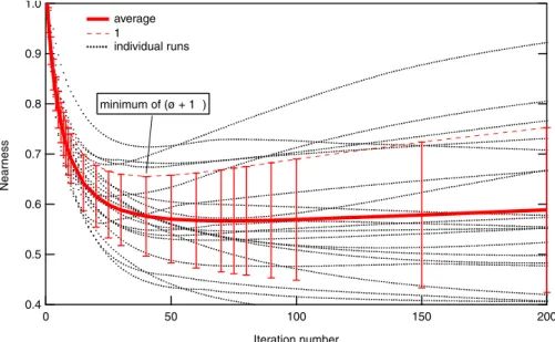
Fig. 5. Minimization in respect to (φ+1σ) of the nearness for one specific test field. The simulation of the measurement and the SIRT reconstruction are applied 1000 times to a single test field with normal distributed measurement errors 1σ=1000 ppb∗m (around 10% relative error). After 40 iterations, the average nearness values still decrease slightly with the iteration number, whereas the scattering of the nearness values increases strongly. As a compromise between a small averageφand a small scattering of the nearness values, the iteration number is chosen that minimizes (φ+1σ ).
4.3.2 Normalized maximum difference (NMD)
The normalized maximum difference (NMD) is the normal-ized maximum absolute value of the reconstruction error.
NMD=N1 max
r∈F 1c(r)
with N= 12
max
r∈F creal(r)−minr∈F creal(r)
(22)
4.3.3 Normalized average difference (NAD)
The normalized average difference (NAD) is the average of the reconstruction error in the area of interest – normalized by the average concentration of the real concentration field. NAD= h1c(r)i
hcreal(r)i
= R
dr21c(r) R
dr2c
real(r)
(23) The NAD is invariant to the multiplication of fields by a scalar factor. This quality criterion is a measure how well the average concentration in the area of interest (and also the total amount of the trace gas species) is reproduced by the reconstruction.
5 Reconstruction optimization
Many parameters are involved in a reconstruction process based on linear discretization and row acting methods:
– dicretization model type (box/bilinear)
– discretization grid size
– first guess of the concentration field
– iteration number of the RAM
All these parameters implicitly add some sort of a priori in-formation. Due to the limited amount of measurement data, the parameters have to be chosen very carefully. Depend-ing on the choice of the discretization model, for example, special kinds of concentration fields are favored.
The optimal set of reconstruction parameters is derived from another kind of a priori information: the assumed prob-ability distribution of the measurement error1dmeasand the
assumed distribution of the random function real concentra-tion fieldcreal(r). The parameters will be optimized so that
the real field will be reconstructed best in average. “Recon-structed best” means, that certain reconstruction quality cri-teria, e.g. the nearness, become minimal. The choice of qual-ity criteria described in the previous section depends on the further use of the reconstructed trace gas map.
5.1 Generation of the set of test plumes
The probability distribution of the random function “real concentration field”creal(r)is realized by a set of test
con-centration fields (ck(r))k∈N. This set is used for
optimiz-ing the reconstruction parameters and estimatoptimiz-ing the error. The aim is to generate random fields in physically reason-able boundaries. It is a compromise between covering all cases and not being too general without need. For this study one hundred test fields were generated by randomly modify-ing the CTM BAB II concentration field (see Fig. 4).
The following modifications which are a coarse represen-tation of physical processes where chosen:
– log-normal distributed random squeeze in intensity (dif-ferent source strength).
– log-normal distributed random squeeze in position space (different meteorological situations).
– normal distributed random shift in position (different meteorological situations and chemistry) .
– addition of a small scale random field (local fluctuations and emissions from other sources).
5.2 Parameter optimization procedure
To find an optimum set of parameters the following numeri-cal experiment was used:
FOR ALL sets of parameters DO {LOOP C} {
FOR ALL test fields ckDO {LOOP B} {
simulate measurement by forward modeling the data from the continuous field;
FOR n random meas. errors DO {LOOP A} {
add measurement error to data;
reconstruct state vector s and related concentration field c(s, r);
evaluate reconstruction quality criteria;
}
evaluateφ+1σ
}
evaluatehφ+1σi;
}
choose set of parameters minimizinghφ+1σi;
As we will see from the numerical experiments, the optimum parameters depend on the size of the measurement errors. For illustrating the optimization procedure we use quality criterion “nearness” (Sect. 4.3.1.).
LOOP A:
1.0
0.9
0.8
0.7
0.6
0.5
0.4
Near
ness
500 400
300 200
100 0
Iteration discretization type
box basis fct. bilinear basis fct.
resolution 3x2 4x3 5x4
1.0
0.9
0.8
0.7
0.6
0.5
0.4
Near
ness
500 400
300 200
100 0
Iteration
simulated meas. error σ = 0ppb*m σ = 100 ppb*m σ = 400 ppb*m σ = 1000 ppb*m
minimum of <ø + 1σ>
(a)
(b)
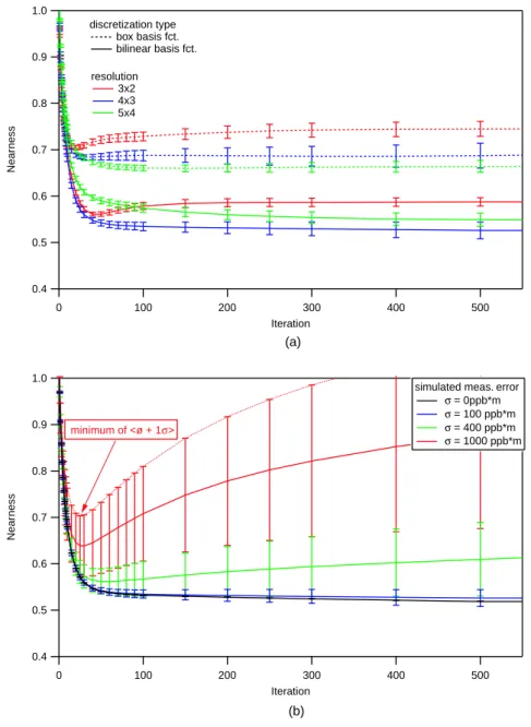
Fig. 6.Parameter optimization. The simulation of a measurement and the SIRT reconstruction are applied on 100 test-fields. The average nearness and its standard deviation averaged over all test-fields are plotted against the iteration number. The standard deviation shows the effect of the propagated measurement error on the nearness. In(a)different state models are compared for fix measurement error σ=100 ppb∗m. For all resolutions the bilinear discretization model is superior to the box model. The 4×3 grid leads to better results than the 3×2/5×4 grids which correspond to strongly over/under determined problems.(b)For the fixed 4×3 bilinear state model the measurement errors are varied from 0–1000 ppb∗m (around 0–10% relative error). The optimum iteration number is determined by minimizing<φ+1σ >. It is highly dependant on the measurement error and decreases when the simulated measurement error increases.
only one test field the optimum iteration number would be the one which minimizes (φ+1σ ). In Fig. 5, for example 40 iterations are optimal.
LOOP B:
Averaging over the set of test fields is done by storing the average of (φ+1σ )over all fields:hφ+1σi.
LOOP C:
Table 1.Results of the procedure for comparing reconstruction methods and inversion parameters. The optimization procedure was applied to the motorway setup used during the BAB II campaign. For different discretization models and inversion techniques the optimum iteration number i is given with respect to the three quality criteria nearness, normalized average difference (NAD), and normalized maximum difference (NMD). We took the optimum iteration number i for a minimum average plus one standard deviation of the quality criteria, thus making a compromise between the value of a quality criteria and its scattering of a quality criteria. The upper part of the table compares different discretization models for the fixed SIRT algorithm. The lower part compares different inversion techniques and their ideal iteration number depended on the assumed measurement error. In this part of the table the discretization model is fixed to be “4×3 bilinear”.
Meas. Err. RAM. Disc. Grid- Nearness NAD NMD
σmeas mod. size < 8+1σ >min 1σ i < 8+1σ >min 1σ i < 8+1σ >min 1σ i
100 SIRT box 3×2 0.71 4.84E-03 20 0.0103 0.0064 40 0.64 7.66E-03 150
100 SIRT Bil 3×2 0.57 4.30E-03 40 0.0114 0.0063 40 0.53 7.86E-03 2000
100 SIRT box 4×3 0.69 4.85E-03 30 0.0206 0.0157 1000 0.60 8.04E-03 40
100 SIRT Bil 4×3 0.53 8.83E-03 100 0.0130 0.0091 400 0.47 1.36E-02 500
100 SIRT box 5×4 0.67 6.02E-03 100 0.0309 0.0073 2000 0.58 1.13E-02 200
SIRT Bil 5×4 0.56 1.43E-02 500 0.0218 0.0076 250 0.45 1.86E-02 1000
100 ART Bil 4×3 0.56 1.58E-02 10 0.0174 0.0136 30 0.49 1.24E-02 4
1000 ART Bil 4×3 0.84 0.1102404 1 0.1029 0.0778 6 0.60 8.51E-02 2
100 SART Bil 4×3 0.54 1.51E-02 40 0.0093 0.0063 6 0.47 1.54E-02 100
1000 SART Bil 4×3 0.75 6.26E-02 4 0.0626 0.0614 6 0.62 0.070997 10
100 SIRT Bil 4×3 0.53 8.83E-03 100 0.0130 0.0091 400 0.47 1.36E-02 500
1000 SIRT Bil 4×3 0.70 6.47E-02 25 0.0716 0.0597 80 0.58 7.78E-02 50
5.3 Parameter optimization for the motorway setup The numerical optimization procedure was applied to the measurement setup used during the BAB II campaign (Fig. 1a). As first guess a constant field with the average concentration of the measured light-paths was used which proved to be suitable in preliminary examinations. Some op-timization results for different quality criteria are presented in Table 1. For different discretization models and types of row acting methods the optimum iteration number is given. As we were interested in the overall shape of the plume, we decided to employ the quality criterion “nearness” for the rest of this study. The optimization is graphically illustrated in Fig. 6. In Fig. 6a the Nearness is plotted against the it-eration number for different state models using the SIRT-algorithm. The bilinear discretization model is superior to the box model because of the smaller discretization error. The combination of a simultaneous row acting method and a bilinear discretization model on a 4×3 grid seems to be best. In Fig. 6b the dependence of the optimal iteration number on the measurement error is demonstrated. If the measure-ment error increases, the ideal iteration number decreases. The optimum iteration number in our case is about 100 for a measurement error of 100–400 ppb∗m which is about 2% relative error and corresponds to the measurement error dur-ing the motorway campaign. In spite of the optimization, all nearness values are relatively high, as the source region above the carriageway where large concentration gradients occur is poorly covered by the light paths. This problem can be seen more clearly in the 2-D error fields and reconstructed concentration fields of the next sections.
5.4 General observations
Applying the optimization procedure to different measure-ment setups (motorway campaign and other atmospheric se-tups) the following general observations were made:
– As discretization model the bilinear interpolation model is superior to the box model.
– Comparing the reconstruction quality of different row acting methods, the SIRT-like inversion method was best in the presence of noise on the data, closely fol-lowed by SART. The ART-like method yielded dis-tinctly worse results.
– The convergence is much faster for SART than for SIRT, but in our case this is not of interest because both algo-rithms are very fast for our problem size.
– If the grid size is optimal the inverse problem is only just or just not anymore well determined. In other words the resolution matrixR=F†Fwhich should be close to unity is nearly of full rank. If the grid size is smaller the discretization error gets large and the result gets worse.
6 Reconstruction results
Table 2. Optimized reconstruction parameters for the motorway campaign.
Discretization model 4×3 bilinear
RAM type simult. iterative projection method
First guess constant average
Iteration Number 100
cycle which reached 1500 m–2000 m altitude. On synaptic scales the pressure differences were small; therefore the ad-vective processes were not dominating.
For reducing the stepping error the NO2 data from the BAB II-campaign had to be averaged over several hours. Be-cause of the linearity of the reconstruction process (in the inversion process each projection of the row acting method is linear and the state model is linear), this averaging of the data equals averaging the 2-D-concentration fields. There-fore the reconstructed fields are time-average concentration fields over the selected periods. The problem of temporal changes of the concentration field during one stepping cycle which result in stepping errors is discussed in the next sec-tion.
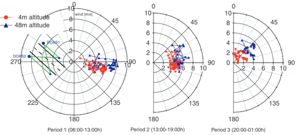
Searching time periods in which the wind direction is approximately perpendicular to the motorway and taking into account the measurement periods of the IMK-Karlsruhe we chose three time periods.
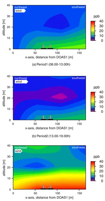
Period 1 10 May 2002 06:00–10 May 2002 13:00 CET Period 2 10 May 2002 13:00–10 May 2002 19:00 CET Period 3 10 May 2002 20:00–11 May 2002 01:00 CET Figure 7 shows the reconstructed NO2 concentration fields for the three time periods. We used the recon-struction parameters optimized for this setup, as listed in Table 2. The shape of the exhaust gas plume depends on the strength of the source (vehicle flux), the chemistry, the wind-speed, the wind-direction and the atmospheric stratification. During situations with stable stratification the exhaust gas concentrations increase strongly – especially if the wind speed orthogonal to the motorway is low. Because the main sources of NO2 at the motorway are chemical reactions and not direct emission, the concentration maxi-mum is on the downwind side of the motorway. The IMK Karlsruhe performed measurements of the vertical wind and temperature profiles during the campaign (M. Kohler, personal communication). The wind vectors measured at two different altitudes are shown in Fig. 8. The shape of the reconstructed plumes agrees with expectations based on vehicle fluxes (B. Vogel, personal communication) and meteorological conditions. Time period 1 (Fig. 7a) includes
M
ppb
0 10 20 30 40
(a) Period1 (06.00-13.00h)
ppb
0 10 20 30 40
(b) Period2 (13.00-19.00h)
ppb
0 10 20 30 40
(c) Period3 (20.00-01.00h)
wind
wind
wind
northeast southwest
0 50 100 150
0 10 20 30 40
x-axis, distance from DOAS1 [m]
altitude [m]
northeast southwest
0 50 100 150
0 10 20 30 40
x-axis, distance from DOAS1 [m]
altitude [m]
northeast southwest
0 50 100 150
0 10 20 30 40
x-axis, distance from DOAS1 [m]
altitude [m]
Fig. 7. Reconstruction results for the BAB II campaign. The re-construction was performed using the simultaneous row acting in-version method and a 4×3 bilinear interpolation model (SIRT-like). The reconstructed concentration fields are in good agreement with the meteorological situation. During day time the exhaust gases were driven away from the carriageway by a soft breeze. Due to the morning rush hour the plume is stronger in period 1. At nighttime the wind-speed at ground-level was almost zero and the temperature gradient showed an inversion situation which leads to high concen-trations (also in the background air).
0 2 4 6 8 10
2 4 6 8 10
0
45
90
135
180 0
2 4 6 8 10
2 4 6 8 10
0
45
90
135
180 225
270 315 4m altitude 48m altitude
0 2 4 6 8 10
2 4 6 8 10
0
45
90
135
180 DOAS1
DOAS2
wind [m/s]
Period 1 (06:00-13:00h) Period 2 (13:00-19:00h) Period 3 (20:00-01:00h)
Fig. 8.Wind direction BAB II. The wind direction at 4 and 50 m altitude above the motorway is plotted for the three time periods. The wind component vertical to the motorway is the smallest during time period 3.
60x103 50 40 30 20 10 0 -10
column density [ppb*m]
09:00 12:00 15:00 18:00 21:00 00:00 time CET
data point dtk and 1σ error bars smoothing spline f(t)
estimated error dtk-f(tk)
Fig. 9.Estimation of the stepping error. The scattering of the mea-surement data is not primarily due to insufficient meamea-surement de-vices, but to real atmospheric and vehicle emission fluctuations dur-ing the steppdur-ing process. The measured NO2slant column densities (red) for one lightpath are plotted against the time. The stepping er-ror of an individual data point (blue) is estimated to be its distance from an interpolating smoothing spline (green).
Consequently, the NO2concentrations are distinctly lower. In both periods (1 and 2) the plume is driven away to the right of the carriageway by a soft breeze.
During time period 3 (Fig. 7c) the ground wind speed gets very slow. Together with a stable stratification and thus a very low boundary layer this leads to a strong accumulation of NO2. In this time period, at around 40 m altitude, concen-trations 5–10 ppb higher than the background concentration were reconstructed. Because no lightpath is crossing this up-per area (see Fig. 4a) this feature is likely to be an artifact of
the reconstruction. By considering the reconstruction error which is quantified in the following section the lack of sig-nificance of this feature is confirmed. Also the exact position of the plume maximum cannot be determined well with this measurement setup as one can see in the error maps Fig. 10a, b, Fig. 11a and Fig. 12a, c. which are described in Sect. 7. For instance it is possible that the real maximum in period 1 and 2 is located closer to the motorway.
It is interesting to note that the plume shapes and con-centration values correspond well to the simulated NO2 pro-files of B¨aumer (2003). In his simulations for the same mo-torway situation, emission data and wind data from a for-mer campaign were used. The results of his simulations for 13:00 CET (unstable stratification) show similar features (plume height, absolute concentration) as our reconstructions from period 1/2, the ones for 21:00 CET (stable stratification) as period 3.
7 Estimated reconstruction error
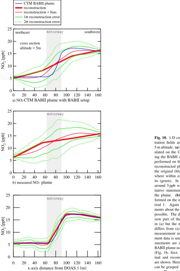
After sketching the determination of the measurement error on the data, our procedure for estimating the measurement error and the discretization + inversion error are described. Resulting 1-D cross sections and 2-D error maps are pre-sented for the real data and the CTM BAB II plume, also with an improved motorway measurement setup.
7.1 Stepping error
25
20
15
10
5
0
NO
2
[ppb]
160 140 120 100 80 60 40 20 0
CTM BABII plume reconstruction reconstruction + bias 1σ reconstruction error 2σ reconstruction error
northeast
cross section altitude = 5m
southwest
25
20
15
10
5
0
NO
2
[ppb]
160 140 120 100 80 60 40 20 0
25
20
15
10
5
0
NO
2
[ppb]
160 140 120 100 80 60 40 20 0
x-axis distance from DOAS 1 [m]
motorway motorway motorway
a) NO2 CTM BABII plume with BABII setup
b) measured NO2 plume
c) NO2 CTM BABII plume with enhanced setup
ppb
0.0 0.2 0.4 0.6 0.8
M
ppb
0.0 0.2 0.4 0.6 0.8
northeast southwest
0 50 100 150
0 10 20 30 40
x-axis, distance from DOAS1 [m]
northeast southwest
0 50 100 150
0 10 20 30 40
x-axis, distance from DOAS1 [m]
altitude [m]
(a) std. dev. map , original setup (b) std. dev. map , enhanced setup
Fig. 11.Measurement error. Subfigure(a)shows the propagated measurement error for the BAB II setup at time period 1. The error is the largest close to the carriageway. This is due to the poor coverage of this region with light beams. The shifting to the right results from higher fluctuations of the concentrations and thus a higher absolute measurement error on the right hand side of the motorway in this wind situation. Subfigure(b)shows the measurement error map for the enhanced motorway setup. The error on the data was assumed to be the same for all light paths and of average size of the errors in subfigure (a). One must be careful in comparing (a) and (b) as the choice of taking the same error for all light paths in (b) already results in a smoother and more symmetric field. Independent of the spatial distribution the average resulting error is smaller than in (a) because more light paths are in the area.
light paths. If the observed concentration field shows tempo-ral fluctuations, e.g. if vehicles are passing the measurement site, then the measurement data scatters around the average. This scattering produces the stepping error. The stepping error can be reduced by averaging the data over a time pe-riod, smoothing or interpolating the data. We averaged the data to get data valuesd. The stepping error was estimated in the following way: The measurement data as a function of time is interpolated with a smoothing spline (IGOR Pro, Wave Metrics, Inc., with reference to Reinsch, 1967) where for each measurement point its measurement error derived from the DOAS analysis is taken into account. The smooth-ness parameter of the interpolation method was chosen by eye. The distance of the measurement data from the inter-polating spline is taken as the stepping error of a single data point. From this the standard error of the mean is calculated:
d= 1
K
K
X
k=1
dt k; 1d =
s PK
k=1(dtk −f (tk))2
(K−1)K , (24) wheredt kare the data points at timetk,f (t )is the
interpolat-ing spline curve andKis the sample size of the period to be averaged. The stepping error was estimated separately for all light paths. In Fig. 9 this estimation is shown for one light-path. The measured slant column densities, the interpolated spline and the resulting estimated errors for each single point are plotted. The resulting relative error for the lightpaths was about 2% of the average column densities.
7.2 Propagated measurement error
We assume that the measurement error on the data, which in our case is the stepping error described in the previous
section, is independent and Gaussian distributed. Then we can calculate the measurement error in the reconstruction 1cmeas(r)from the covariance of the measurement error on
the datacovdmeas with Eq. (18) from Sect. 4.2. The
diago-nal elements ofcovdmeas correspond to the stepping errors.
Fromcovcmeas a standard deviation map is obtained which
gives an impression about the insecurity of the reconstruction at different points due to the measurement error on the data. 7.3 Discretization and inversion error
As described in Sect. 4.2. we estimate the discretization + inversion error by a numerical experiment which corre-sponds to Eq. (17). We simulate the measurement and the reconstruction on a set of test fields (ck(r))k∈N which are
described in Sect. 5.1. They are based on the CTM-BABII plume (B¨aumer pers. comm.) which is shown in Fig. 4a. The difference between the resulting concentration fields and the test fields,1ck(r), is evaluated statistically to get the error
fields:
h1cdii(r)=
1 k
K
X
k=1
1ck(r) (25)
σ (1cdi)(r)=
v u u t 1 K
K
X
k=1
(1ck(r)2− h1cdii(r)) (26)
The distribution of the discretization and inversion error 1cdi(r)is not symmetric around zero. Therefore we always
show the average maph1cdii(r)and the standard deviation
mapσ (1cdi)(r)to get an impression about the quality of the
(c) std. dev. map , original setup
M
ppb
-5.0 -2.5 0.0 2.5 5.0
M
ppb
-5 -2.5 0.0 2.5 5.0
M
ppb
0 2 4 6 8
M
ppb
0 2 4 6 8
northeast southwest
0 50 100 150
0 10 20 30 40
x-axis, distance from DOAS1 [m]
northeast southwest
0 50 100 150
0 10 20 30 40
x-axis, distance from DOAS1 [m]
altitude [m]
(a) average map <Dcdi>, original setup
northeast southwest
0 50 100 150
0 10 20 30 40
x-axis, distance from DOAS1 [m]
northeast southwest
0 50 100 150
0 10 20 30 40
x-axis, distance from DOAS1 [m]
altitude [m]
(d) std. dev. map , enhanced setup (b) average map <Dcdi>, enhanced setup
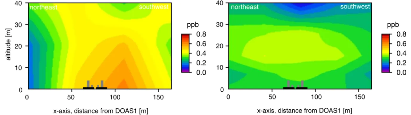
Fig. 12.Discretization and inversion error. The combination of discretization and inversion error was determined by a numeric experiment with a set of test plumes based on the CTM BAB II plume for the north-east wind situation. This error is not symmetric around zero, therefore we plot the average(a, b)and the std. dev.(c, d)of the error distribution. Subfigure (a) and (c) refer to the original setup. (a) The concentration is underestimated where high concentration values are likely, but overestimated in the other regions: The plume is smoothed, because the discretization model is too low resolved and cannot represent the steep concentration gradient which is likely to occur over the motorway. (c) The standard deviation is the highest above the road, because the coverage with light beams is insufficient, and smallest on the sides of the road where a lot of light beams are available. For the enhanced setup the average deviation (b) is generally low (ignoring the area high above the road, which is not of scientific interest). The standard deviation (d) exceeds 2 ppb only in the lowest 2 m above the carriageway. Because of the traffic no light beams could be located here.
7.4 1-D cross-sections of concentration fields
Before discussing the 2-D-error maps we present 1-D cross sections of these maps. The plots in Fig. 10 show hori-zontal NO2concentration cross-sections perpendicular to the carriageway, 5 m above ground. Additionally the 1σ and 2σ reconstruction error limits are plotted. They are de-rived by adding the average and the standard deviation of the estimated error1c(r)to the reconstruction result. It was tested in a numerical experiment that in the given situation adding up the standard deviations of1cmeas(r)and1cdi(r)
quadratically is a good approximation for folding the distri-butions.
For Fig. 10a a theoretical measurement was simulated on the CTM BAB II plume and the concentration distribution reconstructed from the column densities. The uncertainty of the concentration in the middle area and therefore the
differ-ence between the original and its reconstruction is high. This is due to the missing coverage of lightbeams directly above the carriageway on the one hand and the high concentration gradients near the source on the other hand. The a priori in-formation which is implicitly used in the underdetermined region smoothes the result. Another reason for the differ-ence is that the 4×3 bilinear interpolation model, which can be recognized by the four sharp bends of the reconstructed curve, cannot grasp the CTM BAB II plume.
In Fig. 10b we show the cross section of the NO2 concen-tration at time period 1 (taken out of the 2-D field Fig. 7a). The estimated reconstruction error consists of the same dis-cretization and inversion error part 1cdi(r) as in Fig. 10a
reconstruction quality is good enough to determine qual-itatively a “plume type” like “evening inversion plume” or “strong wind plume”. For quantitative statements this measurement setup works only in the areas of the verti-cal profiles on both sides. One might have the idea, that (crec(r)+ h1c(r)i)(the fine red curve) is a better estimation
for the real field thancrec(r). This was true, if the a priori
information represented by the set of model plumes was ex-actly right. As we don’t know the reliability of this informa-tion and don’t want to force the reconstrucinforma-tion result towards the CTM BAB II plume which was used to generate the test fields, we don’t pursue this idea.
7.5 2-D error maps
In the error maps Figs. 11 and 12, respectively, the propa-gated measurement error field1cmeas(r), and the
discretiza-tion and inversion error field1cdi(r)are shown separately.
With these maps, the uncertainty can be estimated for each point of the field by adding the two standard deviation error fields statistically and taking the average map <1cdi(r)>
into account.
Additionally to the effects explained in Sect. 7.4 the recon-struction is less accurate directly above the motorway, and more accurate at higher altitude than at five meter (Fig. 10). The standard deviation due to the measurement error (see Fig. 11) – shown for time period 1 – is relatively small com-pared to the other errors. The average maps of1cdi(r)show
that generally the concentrations are underestimated at the lo-cation of the plumes, and overestimated in the other regions. This “watering down” is caused by the discretization error (the state model is not fine enough to describe the plume po-sition accurately) and due to a general smoothing of SIRT at low iteration numbers in underdetermined regions. In our setup the inversion + discretization error due to the few mea-surements is of the order of ten times higher than the propa-gated measurement error.
7.6 Reduced errors with an improved measurement setup The uncertainties of the reconstructions require an improved measurement setup which is able to quantify the plume shape and concentration accurately over the entire field and which can be used for possible future campaigns.
In numerical experiments we added two more DOAS tele-scopes between the existing teletele-scopes and one additional retro reflector on a bridge at 5 m altitude above the motor-way (see Fig. 1b). Instead of conventional telescopes, four multibeam telescopes (a new type of telescope which is able to measure several light paths simultaneously) are used for measuring six light paths simultaneously. These telescopes measure four light paths which are stepping between two retroreflectors, respectively, one fix light path to the bridge retroreflector (passing the most fluctuating part) and one light path for intercalibration purposes. The averaging time, and
hence the time resolution are therefore reduced by a factor of five preserving the actual stepping errors size. The 36 light paths enable us to choose a higher resolved state model. A 6×4 bilinear interpolation model yielded the best reconstruc-tion results with SIRT in the optimizareconstruc-tion process.
For the error studies the data errors were assumed to be identical for all light paths and of average size of the errors of the campaign time period 1. In Fig. 10c the 1-D cross section of the CTM BAB II plume and its reconstruction are shown for the new measurement setup. The difference be-tween the original plume and the reconstruction is smaller than 1 ppb, and the 1σ limits are lower than 2 ppb (even in the problematic central area).
In Fig. 11b and Fig. 12b, c the two types of errors are shown separately on 2-D maps. The asymmetry in the mea-surement error map is due to the slightly asymmetric posi-tion of the retro-reflector towers. Only the lowest two me-ters above the motorway cannot be reconstructed very well as DOAS- light beams cannot be used at this altitude because of the cars. Also the top middle region can’t be well deter-mined by this setup but this area is not so important from the scientific point of view.
8 Conclusions
We have presented a procedure for comparing different re-construction techniques and optimizing the rere-construction parameters for DOAS tomography measurements. The sim-ulations of the measurement and the reconstruction were ap-plied to a set of test plumes for different combinations of reconstruction techniques and parameters to find the opti-mal reconstruction algorithm and set of parameters. The set of test plumes represent all concentration fields which are physically reasonable according to our a priori informa-tion. For judging the reconstruction quality the quality cri-terion “nearness” was used in this study. For other purposes we suggested the criteria “normalized maximum difference” (NMD) and “normalized average difference” (NAD).
We used the procedure for comparing different row acting methods (ART-, SIRT-, and SART-like) and two types of dis-cretization models (box, bilinear interpolation). The proce-dure can also be employed to optimize measurement setups. In the presence of noise on the data, an extension of the si-multaneous iterative projection method SIRT with a bilinear discretization model yielded the best reconstruction results. The SART algorithm was slightly inferior and the ART-like inversion method, came off distinctly worse.