Inversion of tropospheric profiles of aerosol extinction and HCHO and NO<sub>2</sub> mixing ratios from MAX-DOAS observations in Milano during the summer of 2003 and comparison with independent data sets

(1)

AMTD

4, 3891–3964, 2011

Inversion of tropospheric profiles

from MAX-DOAS

T. Wagner et al.

Title Page

Abstract Introduction

Conclusions References

Tables Figures

◭ ◮

Back Close

Full Screen / Esc

Printer-friendly Version Interactive Discussion

Discussion

P

a

per

|

Dis

cussion

P

a

per

|

Discussion

P

a

per

|

Discussio

n

P

a

per

|

Atmos. Meas. Tech. Discuss., 4, 3891–3964, 2011 www.atmos-meas-tech-discuss.net/4/3891/2011/ doi:10.5194/amtd-4-3891-2011

Atmospheric Measurement Techniques Discussions

This discussion paper is/has been under review for the journal Atmospheric Measure-ment Techniques (AMT). Please refer to the corresponding final paper in AMT

if available.

Inversion of tropospheric profiles of

aerosol extinction and HCHO and NO

₂

mixing ratios from MAX-DOAS

observations in Milano during the

summer of 2003 and comparison with

independent data sets

T. Wagner1, S. Beirle1, T. Brauers2, T. Deutschmann3, U. Frieß3, C. Hak4,

J. D. Halla5, K. P. Heue1, W. Junkermann6, X. Li2, U. Platt3, and I. Pundt-Gruber7

1

Max-Planck-Institut f ¨ur Chemie, Mainz, Germany

2

Institute f ür Energie- und Klimaforschung Troposph äre (IEK-8), Forschungszentrum J ülich, J ülich, Germany

3

Institute for Environmental Physics, University of Heidelberg, Heidelberg, Germany

4

(2)

AMTD

4, 3891–3964, 2011

from MAX-DOAS

T. Wagner et al.

Title Page

Tables Figures

◭ ◮

Back Close

Full Screen / Esc

Discussion

P

a

per

|

Dis

cussion

P

a

per

|

Discussion

P

a

per

|

Discussio

n

P

a

per

|

5

Centre for Atmospheric Chemistry, York University, Toronto, ON, Canada

6

Institute for Meteorology and Climate Research, IMK-IFU, Karlsruhe Institute of Technology, Garmisch-Partenkirchen, Germany

7

Johannes-Kepler-Gymnasium, Weil der Stadt, Germany

Received: 22 April 2011 – Accepted: 9 June 2011 – Published: 22 June 2011 Correspondence to: T. Wagner (thomas.wagner@mpic.de)

(3)

AMTD

4, 3891–3964, 2011

from MAX-DOAS

T. Wagner et al.

Title Page

Tables Figures

◭ ◮

Back Close

Full Screen / Esc

Discussion

P

a

per

|

Dis

cussion

P

a

per

|

Discussion

P

a

per

|

Discussio

n

P

a

per

|

Abstract

We present aerosol and trace gas profiles derived from MAX-DOAS observations. Our inversion scheme is based on simple profile parameterisations used as input for an atmospheric radiative transfer model (forward model). From a least squares fit of the forward model to the MAX-DOAS measurements, two profile parameters are retrieved 5

including integrated quantities (aerosol optical depth or trace gas vertical column den-sity), and parameters describing the height and shape of the respective profiles. From these results, the aerosol extinction and trace gas mixing ratios can also be calculated. We apply the profile inversion to MAX-DOAS observations during a measurement campaign in Milano, Italy, September 2003, which allowed simultaneous observations 10

from three telescopes (directed to north, west, south). Profile inversions for aerosols and trace gases were possible on 23 days. Especially in the middle of the campaign

(17–20 September 2003), enhanced values of aerosol optical depth and NO₂ and

HCHO mixing ratios were found. The retrieved layer heights were typically similar for

HCHO and aerosols. For NO₂, lower layer heights were found, which increased during

15

the day.

The MAX-DOAS inversion results are compared to independent measurements: (1)

aerosol optical depth measured at an AERONET station at Ispra; (2) near-surface NO₂

and HCHO (formaldehyde) mixing ratios measured by long path DOAS and Hantzsch instruments at Bresso; (3) vertical profiles of HCHO and aerosols measured by an ultra 20

light aircraft. Depending on the viewing direction, the aerosol optical depths from MAX-DOAS are either smaller or larger than those from AERONET observations. Similar

comparison results are found for the MAX-DOAS NO₂ mixing ratios versus long path

DOAS measurements. In contrast, the MAX-DOAS HCHO mixing ratios are generally higher than those from long path DOAS or Hantzsch instruments. The comparison of 25

(4)

AMTD

4, 3891–3964, 2011

from MAX-DOAS

T. Wagner et al.

Title Page

Tables Figures

◭ ◮

Back Close

Full Screen / Esc

Discussion

P

a

per

|

Dis

cussion

P

a

per

|

Discussion

P

a

per

|

Discussio

n

P

a

per

|

different telescopes, it was possible to investigate the internal consistency of the

MAX-DOAS observations.

As part of our study, a cloud classification algorithm was developed (based on the

MAX-DOAS zenith viewing directions), and the effects of clouds on the profile inversion

were investigated. Di_fferent e_ffects of clouds on aerosols and trace gas retrievals were

5

found: while the aerosol optical depth is systematically underestimated and the HCHO

mixing ratio is systematically overestimated under cloudy conditions, the NO₂ mixing

ratios are only slightly a_ffected. These findings are in basic agreement with radiative

transfer simulations.

1 Introduction

10

MAX-DOAS instruments measure scattered sun light from di_fferent, mostly slant

eleva-tion angles, thus having a high sensitivity to trace gases and aerosols located close to the Earth’s surface (e.g., H ¨onninger et al., 2002; Van Roozendael et al., 2003; Wittrock et al., 2004; Wagner et al., 2004; Brinksma et al., 2008 and references therein). In addition to the retrieval of trace gas mixing ratios or aerosol extinction close to the sur-15

face, information on vertical profiles and vertically integrated quantities (vertical trace gas column density, VCD, or aerosol optical depth, AOD) can be retrieved.

In recent years, several algorithms for the quantitative retrieval of trace gas and aerosol properties from MAX-DOAS observations have been developed and applied by

di_fferent research groups (e.g., Heckel et al., 2005; Irie et al., 2008; Cl ´emer et al., 2010;

20

Li et al., 2010), and also some comparison studies with independent data sets have been performed (Heckel et al., 2005; Irie et al., 2008; Cl ´emer et al., 2010; Li et al., 2010; Zieger et al., 2011). Currently, the development and application of profile retrieval algo-rithms for MAX-DOAS observations is a very active field of research; recently a com-prehensive measurement campaign with contributions from many research groups 25

(5)

AMTD

4, 3891–3964, 2011

from MAX-DOAS

T. Wagner et al.

Title Page

Tables Figures

◭ ◮

Back Close

Full Screen / Esc

Discussion

P

a

per

|

Dis

cussion

P

a

per

|

Discussion

P

a

per

|

Discussio

n

P

a

per

|

Nitrogen Dioxide measuring Instruments, CINDI, http://www.knmi.nl/samenw/cindi/) (see Roscoe et al., 2010 and references therein).

Usually MAX-DOAS inversion algorithms use a two-step approach: in the first step, aerosol extinction profiles are retrieved from the measured absorption of the oxygen

dimer O₄(e.g., Heckel et al., 2005; Sinreich et al., 2005; Li et al., 2010; Cl ´emer et al.,

5

2010). In a second step, trace gas profiles are retrieved from the measured trace gas absorptions, taking into account the aerosol properties retrieved in the first step.

The information content of MAX-DOAS observations in the UV is typically limited to 2–3 independent pieces of information for the retrieved vertical profiles (see Frieß et al., 2006; Cl ´emer et al., 2010). Most inversion algorithms are based on the optimal 10

estimation method making explicit use of a-priori profiles and associated uncertainties (Rodgers, 2000). In this study we apply a MAX-DOAS inversion algorithm for trace

gases and aerosols, which uses a different strategy and does not include explicit

a-priori profile information and associated uncertainties, but instead assumptions on the relative profile shapes only. This method was recently introduced by Li et al. (2010); 15

here we apply a slightly modified version.

Our forward model uses a simple profile parameterisation scheme with only three parameters (for details see Sect. 3.1), which is used as input for a radiative transfer model. The actual profile inversion process consists of a least squares fit of the forward model results to the results of the MAX-DOAS measurement. The fit yields the profile 20

parameters (and associated uncertainties), which fit best to the measurements. One general problem with all inversion algorithms for MAX-DOAS observations is

the di_fficulty to accurately determine the errors of the profile inversion results. This

dif-ficulty is caused by several reasons. First, the information content of the measurement is limited and thus only averaged quantities (e.g. the average trace gas concentration 25

for a specified layer) can be retrieved. Second, ambiguities arise because in principle

quite di_fferent atmospheric profiles could cause similar MAX-DOAS results. Third,

(6)

AMTD

4, 3891–3964, 2011

from MAX-DOAS

T. Wagner et al.

Title Page

Tables Figures

◭ ◮

Back Close

Full Screen / Esc

Discussion

P

a

per

|

Dis

cussion

P

a

per

|

Discussion

P

a

per

|

Discussio

n

P

a

per

|

the results of the aerosol profile inversion (first step of the profile inversion). Fourth, simplified assumptions are used in the forward model, e.g. horizontal homogenous dis-tributions. However, in reality horizontal gradients and transport of air masses might

exist, which affect the MAX-DOAS retrievals. Fifth, the measurements can be affected

by systematic errors (e.g. wrong trace gas absorption cross sections, wrong aerosol 5

optical properties, wrong adjustments of the telescopes, or the presence of clouds). Due to all of these reasons, deriving a reliable error estimation from the MAX-DOAS

inversion process is di_fficult. Here it should be noted that this is also true for retrievals

using optimal estimation. One important way to quantify the errors is thus validation by the results of independent measurements.

10

In this study we apply our profile inversion algorithm to MAX-DOAS observations during the FORMAT campaign in Milano (Italy) in late summer 2003 (for details see Sect. 2). Note that an initial study on MAX-DOAS retrievals for a limited period was already conducted by Heckel et al. (2005) and Wittrock (2006). Measurements during the FORMAT campaign are well suited to assess the accuracy of the profile retrieval, 15

because several independent measurements are available for comparison: HCHO

and NO₂ mixing ratios were measured by a long path (LP-) DOAS instrument (see

Sect. 2.1); HCHO was also measured by a Hantzsch instrument at ground. Vertical profiles of HCHO and aerosol concentrations are available from observations from an ultra light aircraft (see Sect. 2.2). AOD was measured by a sun photometer at the 20

AERONET station at Ispra (http://aeronet.gsfc.nasa.gov/new web/index.html, also see Holben et al. 2001).

Another advantage of the MAX-DOAS instrument used in this study is that

simulta-neous measurements are performed from three di_fferent azimuth directions. From the

comparison of the respective results, information on the consistency of our inversion 25

algorithm can be obtained.

In this study we also investigated the e_ffects of clouds on the MAX-DOAS

obser-vations. We developed a cloud discrimination scheme, which is based on the O₄

(7)

AMTD

4, 3891–3964, 2011

from MAX-DOAS

T. Wagner et al.

Title Page

Tables Figures

◭ ◮

Back Close

Full Screen / Esc

Discussion

P

a

per

|

Dis

cussion

P

a

per

|

Discussion

P

a

per

|

Discussio

n

P

a

per

|

measurement conditions can be discriminated: clear sky conditions, “thin” clouds, and “thick” clouds. Based on this scheme, the MAX-DOAS observations during the

FOR-MAT campaign are classified, and the e_ffects of clouds on the MAX-DOAS observations

are investigated. Cloud effects are also simulated by radiative transfer modeling.

The paper is organised as follows with in Sect. 2 an overview of the measurement 5

campaign. In Sect. 3 the MAX-DOAS inversion algorithm is described. Section 4

dis-cusses the basic effects of clouds on MAX-DOAS observations and introduces the

cloud discrimination scheme. Section 5 presents selected retrieval results and a sys-tematic comparison to independent measurements. In Sect. 6 the main findings are summarised.

10

2 FORMAT 2003 campaign

We investigate MAX-DOAS observations performed in September 2003 during the FORMAT-II campaign (“Formaldehyde as a tracer for oxidation in the troposphere”, see www.nilu.no/format/). The FORMAT project focused on measuring, modelling and interpreting HCHO in the heavily polluted region of the Po-Valley in Northern Italy (see 15

e.g., Hak, 2006; Liu et al., 2007; Junkermann, 2009). During the campaign various

in-situ and remote sensing measurements were performed at different ground-based

stations in the region of Milano and from di_fferent aircraft-based instruments. The

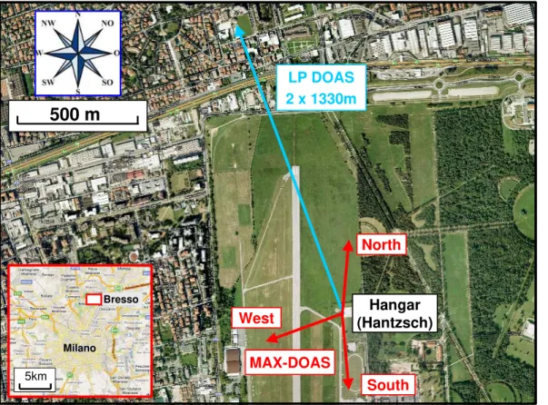
MAX-DOAS measurements used in this study were made at Bresso (45.5◦N, 9.2◦E,

located in the northern part of Milano, Italy) from 4 to 26 September 2003. The re-20

sults of the MAX-DOAS measurements are compared to the results from two other

instruments also located at Bresso: NO₂ and HCHO mixing ratios from a long path

DOAS (LP-DOAS) instrument (Hak, 2006) and HCHO mixing ratios from a Hantzsch instrument (Junkermann, 2009). The locations and viewing directions of these in-struments, along with the MAX-DOAS, are shown in Fig. 1; the instrumental details 25

(8)

AMTD

4, 3891–3964, 2011

from MAX-DOAS

T. Wagner et al.

Title Page

Tables Figures

◭ ◮

Back Close

Full Screen / Esc

Discussion

P

a

per

|

Dis

cussion

P

a

per

|

Discussion

P

a

per

|

Discussio

n

P

a

per

|

depth observations from the AERONET station at Ispra (45.8◦N, 8.6◦E), about 50 km

north-west of Bresso (http://aeronet.gsfc.nasa.gov/new web/index.html, also see

Hol-ben et al. 2001). During the FORMAT-II campaign, three periods with different weather

conditions can be distinguished: before 15 September and after 22 September, vari-able conditions prevailed, while between 15 and 22 September a period with stvari-able 5

conditions, clear skies, and relatively high temperature occurred (Steinbacher et al., 2005a; Hak, 2006; Junkermann, 2009).

2.1 Long path DOAS

With the active Long Path DOAS (LP DOAS) instrument, trace gases present along a defined absorption path can be measured. The LP DOAS applies a 500 W Xenon 10

high-pressure lamp as artificial broad-band light source. Absolute concentrations can be determined from the measured column densities by knowing the length of the ab-sorption path between the sending and receiving telescope (see Platt and Stutz, 2008) and an array of retro reflectors.

During the FORMAT II campaign, long path DOAS systems of di_fferent types were

15

applied at three different sites (Hak et al., 2005; Hak, 2006). At Bresso, an instrument

capable of simultaneously transmitting and receiving multiple light beams was used (see Pundt and Mettendorf, 2005 for details). The data used here was obtained from a light beam directed to a church 1330 m north of the measuring site. The measure-ments cover the wavelength range 283–372 nm. The spectra integration time was typi-20

cally between 40 and 100 s. The absorption spectra were evaluated in the range 300– 360 nm, applying the DOAS method (Platt and Stutz, 2008). The accuracy of a DOAS measurement is influenced mostly by the accuracy of the used reference cross-section

of the investigated species, i.e.∼6 % for HCHO and∼4 % for NO₂. For the LP DOAS

measurements, the detection limits for formaldehyde and nitrogen dioxide during the 25

(9)

AMTD

4, 3891–3964, 2011

from MAX-DOAS

T. Wagner et al.

Title Page

Tables Figures

◭ ◮

Back Close

Full Screen / Esc

Discussion

P

a

per

|

Dis

cussion

P

a

per

|

Discussion

P

a

per

|

Discussio

n

P

a

per

|

2.2 Hantzsch

The Hantzsch technique is based on a sensitive liquid phase detection following a tinuous transfer of HCHO from ambient air into a washing solution in a temperature con-trolled stripping coil. A reaction with 2,4-pentanedione (i.e. acetylacetone) in

ammo-nium acetate bu_ffer solution forms 3,5-diacetyl 1,4-dihydrolutidine (DDL), which can be

5

detected with high sensitivity by fluorescence (Kelly and Fortune, 1994). The technique is the basis for a commercial instrument: AL4001 (AERO-LASER GmbH,

Garmisch-Partenkirchen, Germany) having a detection limit of<50 ppt and a time resolution of

90 s. The accuracy and precision are indicated as ±15 % or 150 pptv and ±10 % or

150 pptv, respectively (Hak et al., 2005). These instruments were used for ground-10

based measurements at three field sites during FORMAT. Additionally an upgraded lightweight version of the instrument (Junkermann and Burger, 2006) was flown sev-eral days on an ultra light research aircraft to measure the horizontal distribution of formaldehyde in the greater Milano area and its vertical profiles north of Milano up to

∼3000 m a.s.l. For this instrument the acuracy is 10 % or 100 ppt (Junkermann and

15

Burger, 2006). Besides HCHO, also profiles of the aerosol concentration were mea-sured (Junkermann, 2009).

2.3 MAX-DOAS instrument and spectral retrieval

The MAX-DOAS instrument observes scattered sun light from three telescopes, which are connected via glass fibre bundles to a spectrograph with a two dimensional CCD-20

detector (see Wagner et al., 2004, 2009). Before 12 September 2003 all telescopes

were directed towards the south (azimuth angle of 185◦ with respect to north, see

Fig. 1). After 12 September 2003, one telescope continued measurements in southerly

direction, but the others were now directed to north and west (azimuth angles of 5◦and

250◦ with respect to north, respectively). During the whole campaign, each telescope

25

sequentially scanned 5 different elevation angles: 3◦, 6◦, 10◦, 18◦ and 90◦ (zenith);

(10)

AMTD

4, 3891–3964, 2011

from MAX-DOAS

T. Wagner et al.

Title Page

Tables Figures

◭ ◮

Back Close

Full Screen / Esc

Discussion

P

a

per

|

Dis

cussion

P

a

per

|

Discussion

P

a

per

|

Discussio

n

P

a

per

|

measurements cover the wavelength range 320–457 nm with a spectral resolution of about 0.75 nm (FWHM).

The MAX-DOAS spectra were analysed using the DOAS method (Platt and Stutz, 2008), details can be found in Wagner et al. (2004, 2009). From the spectral analysis the integrated trace gas concentration along the atmospheric absorption path, the so 5

called slant column density (SCD) is retrieved. In this study we analyse the DSCDs of

NO₂, HCHO and the oxygen dimer O₄. To remove the strong Fraunhofer lines

dom-inating the measured spectra, another spectrum (preferably with small atmospheric absorptions) is also included in the spectral analysis (usually referred to as Fraunhofer

reference spectrum). Thus, the result of the DOAS analysis represents the difference

10

of the SCDs of the measured spectra and the Fraunhofer reference spectrum, often

referred to as di_fferential SCD or DSCD. There exist two basic choices of Fraunhofer

reference spectra: often a fixed Fraunhofer reference spectrum is used to analyse all measured spectra during a selected period (e.g. a complete measurement campaign). If a fixed reference spectrum is used, the retrieved DSCDs not only represent the ef-15

fects of the different viewing angles, but also the variations of the atmospheric trace gas

concentrations between the time of the measured spectra and the Fraunhofer reference

spectrum. Another choice would be to use the respective 90◦elevation spectra for

in-dividual elevation sequences to analyse the spectra of the same elevation sequence.

For this choice the retrieved DSCD simply represents the effects of the different

view-20

ing geometry and are referred as dSCD_α (withα the elevation angle) in the following

(while DSCD is used in a general sense). dSCD_α can be directly used for the profile

inversion.

In this study we use a fixed Fraunhofer reference spectrum (one for each telescope) for the complete campaign. Thus before the DSCDs of an elevation sequence are used 25

for the profile inversion, the DSCD for the 90◦ measurements of the same elevation

sequence is subtracted to derive the respective dSCD_α(see Sects. 3.4 and 3.5).

(11)

AMTD

4, 3891–3964, 2011

from MAX-DOAS

T. Wagner et al.

Title Page

Tables Figures

◭ ◮

Back Close

Full Screen / Esc

Discussion

P

a

per

|

Dis

cussion

P

a

per

|

Discussion

P

a

per

|

Discussio

n

P

a

per

|

From the retrieved O₄ DSCDs (in contrast to NO₂ and HCHO) so called air mass

factors (AMFs) can be directly calculated. The AMF is defined as the ratio of the SCD and the vertically integrated trace gas concentration (VCD) (see e.g., Solomon et al., 1987):

AMF₌SCD/VCD (1)

5

Since the atmospheric O₂profile is known (it varies slightly with temperature and

pres-sure), the O₄VCD can be calculated from atmospheric temperature and pressure

pro-files (see e.g., Greenblatt et al., 1990). For the O₄VCD at Bresso in this study a value

of 1.3×1043molec2cm−5 was used for the conversion of the O₄SCDs into O₄ AMFs

(see Wagner et al., 2009). The advantage of this conversion is that the measured O₄

10

AMF can be directly compared to the output of the radiative transfer simulations (see Sect. 3.2).

Similar to the definitions of the DSCD and dSCD_α, also a differential AMF (DAMF or

dAMF_α) can be defined:

DAMF₌DSCD/VCD or dAMF_α₌dSCD_α/VCD (2)

15

dAMF_α derived in this way are used for the profile inversion (see Sect. 3.4).

Note that the retrieved O₄AMFs (or DAMF or dAMF_α) were corrected by a constant

factor of 0.75. This correction was found to be necessary to bring model results and measurements under almost aerosol and cloud free conditions into agreement (see Wagner et al., 2009, Cl ´emer et al., 2010). The reason for this correction factor is still 20

not understood.

In contrast to O₄, the atmospheric profiles of NO₂ and HCHO are highly variable,

and the respective VCDs are not known beforehand. Thus no DAMF (or dAMF_α) can

be directly calculated from the DSCDs (or dSCD_α). As will be shown in Sect. 3.5, the

VCDs of NO₂and HCHO are obtained from the profile inversion process.

25

(12)

AMTD

4, 3891–3964, 2011

from MAX-DOAS

T. Wagner et al.

Title Page

Tables Figures

◭ ◮

Back Close

Full Screen / Esc

Discussion

P

a

per

|

Dis

cussion

P

a

per

|

Discussion

P

a

per

|

Discussio

n

P

a

per

|

for. The measurement sensitivity depends on distance from the instrument location, varies with several parameters (e.g. viewing geometry, wavelength, aerosol and trace

gas profiles), and is thus di_fficult to quantify. From radiative transfer simulations we find

that for typical aerosol loads during the FORMAT campaign (AOD≥0.3), the sensitivity

of the MAX-DOAS measurements is e_ffectively restricted to air masses within about

5

5 km distance from the measurement location (in viewing direction).

3 MAX-DOAS inversion algorithm

The inversion scheme used in this study follows a two-step approach as suggested by Sinreich et al. (2005) or Heckel et al. (2005). First an aerosol extinction profile

is determined using the O₄ dAMF_α analysed from the MAX-DOAS observations. In

10

a second step, profiles of trace gas concentrations are determined from the respective

trace gas dSCD_α, also taking into account the aerosol extinction profiles determined in

the first step. For both steps, similar profile parameterisations and inversion strategies are used, which are described in the following sections. Our profile inversion scheme is a modified version of the algorithm originally introduced by Li et al. (2010).

15

3.1 Profile parameterisation

The trace gas and aerosol profiles used in this study are defined by only three param-eters:

(a) VCD or AOD

They describe the vertically integrated profile amounts, i.e. the vertically integrated 20

(13)

AMTD

4, 3891–3964, 2011

from MAX-DOAS

T. Wagner et al.

Title Page

Tables Figures

◭ ◮

Back Close

Full Screen / Esc

Discussion

P

a

per

|

Dis

cussion

P

a

per

|

Discussion

P

a

per

|

Discussio

n

P

a

per

|

(b) Layer height,L

This parameter (sometimes the indexed symbols L_aer, L_tracegas, L_NO₂, or L_HCHO are

used) describes the altitude, below which the trace gas concentration or aerosol ex-tinction is assumed to be constant. The values of the aerosol exex-tinction or trace gas concentration above that layer decrease, depending on the third parameter:

5

(c) Shape parameter,S

The shape parameter describes the relative shape of the aerosol or trace gas profiles

(sometimes the indexed symbolsSaer,Stracegas,SNO₂, or SHCHO are used). For shape

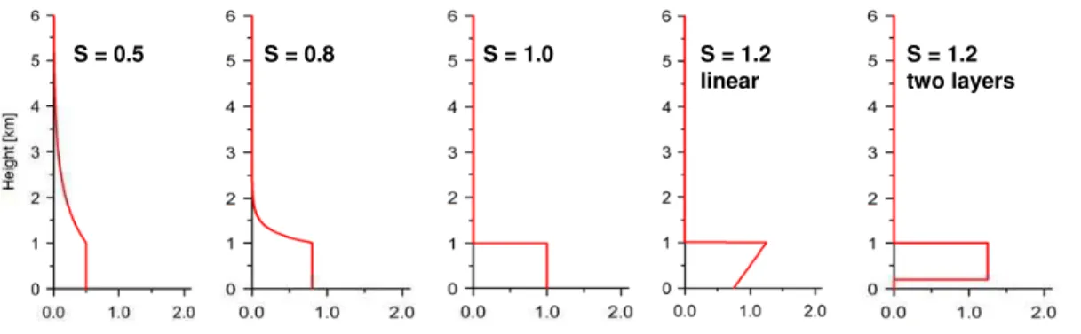
parametersS between 0 and 1, the value ofS describes the fraction of the trace gas

VCD or AOD within the layer (see Li et al., 2010). The remaining fraction is assumed 10

to be located above the layer, where an exponential decrease is assumed (Fig. 2 left). Note that in contrast to Li et al. (2010), who assumed a fixed height parameter for the exponential layer, we use a variable scale height with the boundary condition of a continuous transition of the exponential function at the top of the layer. However, since the sensitivity of MAX-DOAS observations decreases with increasing altitude, these 15

differences have little influence on the profile retrieval. A shape parameter of unity

describes a “box” profile with constant trace gas concentration or aerosol extinction within the layer, and zero above (Fig. 2 center).

3.1.1 Elevated layers

To describe another important type of profiles with increased aerosol extinction or trace 20

gas concentrations at higher altitudes (elevated layers), we extended the range of the

shape parameterSto values>1. Like for shape parametersS <1, a general constraint

is that for S→1, the respective profiles have to merge the box profile (S=1). This

condition is necessary to allow a smooth convergence of the fit.

Elevated profiles probably do not occur very frequently, because most sources of 25

(14)

AMTD

4, 3891–3964, 2011

from MAX-DOAS

T. Wagner et al.

Title Page

Tables Figures

◭ ◮

Back Close

Full Screen / Esc

Discussion

P

a

per

|

Dis

cussion

P

a

per

|

Discussion

P

a

per

|

Discussio

n

P

a

per

|

profiles can occur, if air masses at different altitudes have different origins (e.g. a

resid-ual layers from the previous day). In addition, aerosols or trace gases might be formed from primary pollutants apart from their sources, e.g. in elevated layers by photochem-ical processes (see e.g., Matsui et al., 2010). In such cases, parameterisations for elevated layers are appropriate to describe the corresponding vertical profiles.

5

Several parameterisations for profiles with elevated layers are possible. However, one major problem arises from the fact that according to the limited information content of UV measurements, only up to one shape parameter can be independently deter-mined in the fitting procedure (measurements at additional wavelengths can in principle enhance the information content). One consequence of this limitation is that profile pa-10

rameterisations depending only on one parameter might not be appropriate for di_fferent

situations. For example, a chosen profile parameterisation might be well suited for

spe-cific height profiles, but might fail to describe height profiles for different atmospheric

situations. The advantages and disadvantages of di_fferent possible parameterisations

are briefly described in the following: 15

(a) Linear profiles

The advantage of a linear parameterisation is that profiles with slightly increasing val-ues with altitude can be well described. Such profiles might occur if aerosols or trace gases are produced while their precursors are transported upwards. An important limitation of this parameterisation is that no steep vertical gradients and no vertically 20

extended uplifted layers can be described (e.g. distinct layers with largely differing

av-erage values).

(b) Exponential profiles

Either “convex” of “concave” altitude profiles can be described by exponential param-eterisations. Compared to the linear parameterisations, such parameterisations allow 25

(15)

AMTD

4, 3891–3964, 2011

from MAX-DOAS

T. Wagner et al.

Title Page

Tables Figures

◭ ◮

Back Close

Full Screen / Esc

Discussion

P

a

per

|

Dis

cussion

P

a

per

|

Discussion

P

a

per

|

Discussio

n

P

a

per

|

describe linear profiles at the same time. Exponential profiles with only one parameter have to be optimised for the description of either smooth profiles (quasi linear) or steep vertical gradients (similar to distinct layers). Exponential profiles might thus be interest-ing if two shape parameters could be independently determined in the fittinterest-ing process

(e.g. for measurements using di_fferent wavelengths).

5

(c) Two-layer profiles

In many cases, aerosol profiles with two separate layers (both with independent vertical extension and average aerosol extinction or trace gas concentration) might be a good choice. However, since only up to one shape parameter can be determined by the inversion routine, either the vertical extension or the average value of the second layer 10

has to be kept fixed, while the other parameter could be determined by the inversion process. Both possibilities are well suited to describe distinct layers, but fail if smooth vertical gradients (e.g. linear gradients) have to be described.

In this study, we use two parameterisations for elevated layers (linear profiles and two-layer profiles). For the two-layer profiles we fixed the value of the lowest layer (to 15

zero) but vary the vertical extension of this layer (as described below). Both parame-terisations for elevated layers were chosen, because they describe two extreme cases: extended elevated layers with a sharp gradient at the bottom or smoothly varying pro-files.

For linear profiles, we chose a parameterisation that relates the ratio between the 20

aerosol extinction (or trace gas concentration) at the surfacex_Sand at the layer height

xLto the shape parameter (for 1< S≤1.5) according to the following formula:

x_S/x_L=(1.5−S)·2 (3)

This parameterisation assures that for S→1 the profile merges the box profile. An

example of a linear profile is shown in Fig. 2 (right). 25

(16)

AMTD

4, 3891–3964, 2011

from MAX-DOAS

T. Wagner et al.

Title Page

Tables Figures

◭ ◮

Back Close

Full Screen / Esc

Discussion

P

a

per

|

Dis

cussion

P

a

per

|

Discussion

P

a

per

|

Discussio

n

P

a

per

|

concentration)L_zero and the (total) layer height L to the shape parameter (for S >1)

according to the following formula:

L_zero/L=S−1 (4)

Also this parameterisation assures that forS→1 the profile merges the box profile. An

example of a two-layer profile is shown in Fig. 2 (right). 5

Of course the details of the chosen parameterisations are arbitrary but our profile parameterisation has the advantage that it describes a large variety of possible

pro-files using only 3 parameters including “box” propro-files (S=1), quasi-exponential profiles

(S→0), or profiles with an elevated layer (S >1). However, it should be noted that

this simple parameterisation cannot describe more complex situations like e.g. multiple 10

layers (Frieß et al., 2006; Cl ´emer et al., 2010).

Moreover, it turned out that for some measurement conditions the information

con-tent is not sufficient (e.g. during non-optimum measurement conditions), to determine

all three profile parameters simultaneously, and a stable profile inversion was only pos-sible for 2 profile parameters. In such cases one of the profile parameters introduced 15

above (the shape parameter,S) is set to a fixed value. Because of that finding, in this

study, only two profile parameters were retrieved in order to make a consistent auto-mated retrieval possible. The fact that in some cases no stable retrieval of all three profile parameters was possible, reflects the limited information content of our

MAX-DOAS measurements, for which no measurements at low elevation angles (<3◦) were

20

(17)

AMTD

4, 3891–3964, 2011

from MAX-DOAS

T. Wagner et al.

Title Page

Tables Figures

◭ ◮

Back Close

Full Screen / Esc

Discussion

P

a

per

|

Dis

cussion

P

a

per

|

Discussion

P

a

per

|

Discussio

n

P

a

per

|

3.1.2 Determination of aerosol extinction, trace gas concentration and mixing ratio from the profile parameters

The profile parameters determined from the inversion process directly yield information on the integrated quantities, i.e. the trace gas VCDs or AODs. If shape parameters

S≥1 are used, the height parameter L directly describes the upper boundary of the

5

trace gas or aerosol layer. Also for shape parameters slightly smaller than 1,Lmight

still be a good approximation of the upper boundary of the aerosol or trace gas layer

(for values ofS≪1, however, a correspondingly large fraction (1−S) of the total trace

gas or aerosol amount is located aboveL).

From the derived profile parameters, the average trace gas concentration,ρ, or the

10

average aerosol extinction, ε, within the aerosol or trace gas layer can be derived

according to the following equations (forS≤1):

ε=AOD·S/L (5)

ρ=VCD·S/L (6)

From the average trace gas concentration, also the respective mixing ratioM can be

15

calculated

M=ρ/[air] (7)

For surface mixing ratios a value of the air number density [air] of 2.5×1019molec cm−3

(for 20◦C and 1013 hPa) can be used.

For shape parametersS >1, also aerosol extinction or trace gas concentrations can

20

be derived from the retrieved profile parameters. For the two-layer parameterisation (Eq. 4) the aerosol extinction and trace gas concentration within the elevated layer are derived according to:

ε=AOD·(2−S)/L (8)

ρ=VCD·(2−S)/L (9)

(18)

AMTD

4, 3891–3964, 2011

from MAX-DOAS

T. Wagner et al.

Title Page

Tables Figures

◭ ◮

Back Close

Full Screen / Esc

Discussion

P

a

per

|

Dis

cussion

P

a

per

|

Discussion

P

a

per

|

Discussio

n

P

a

per

|

For the linear profile parameterisation (Eq. 3) the aerosol extinction and trace gas

con-centration as a function of altitude (forz≤L) are derived according to:

ε(z)=AOD

L ·

1₊

_z

L−

1 2

·2(S−1)

(10)

ρ(z)=VCD

L ·

1₊

_z

L−

1 2

·2(S−1)

(11)

As will be shown later, for shape parametersS≤1, the derived trace gas mixing ratios

5

agree well with the independent measurements of near-surface trace gas mixing ratios. Good agreement between aerosol extinction and surface in-situ measurements was also found, as demonstrated in other studies (e.g., Li et al. 2010; Zieger et al., 2011).

3.2 Radiative transfer simulations

For the simulation of trace gas SCDs and AMFs (or dSCD_α and dAMF_α), radiative

10

transfer simulations are performed. The dSCD_α and dAMF_α are calculated as the

difference of simulation results (for the same settings) for the elevation angles α and

90◦. They are expressed as function of the profile parameters introduced in Sect. 3.1;

these relationships establish the forward model:

dAMF_α=f(S_aer,L_aer,AOD,α,SZA,RAA) (12)

15

dSCD_α=f(S_tracegas,L_tracegas,VCD,S_aer,L_aer,AOD,α,SZA,RAA) (13)

HereS_aer,L_aer and AOD are the shape parameter, layer height and total optical depth

of the aerosol profile;S_tracegas,L_tracegasand VCD are the shape parameter, layer height

and vertical column density of the trace gas profiles. α, SZA, RAA are the elevation

angle, solar zenith angle and relative azimuth angle between the telescope and the 20

sun. Note that the forward model for the trace gas dSCD_α also includes the aerosol

profile parameters.

(19)

AMTD

4, 3891–3964, 2011

from MAX-DOAS

T. Wagner et al.

Title Page

Tables Figures

◭ ◮

Back Close

Full Screen / Esc

Discussion

P

a

per

|

Dis

cussion

P

a

per

|

Discussion

P

a

per

|

Discussio

n

P

a

per

|

which is described in detail in Deutschmann (2008), and Deutschmann et al. (2011). For the simulations in this study, a surface albedo of 5 %, aerosol single scattering albedo of 0.95 and aerosol asymmetry parameter of 0.68 are assumed, which are typ-ical values for urban and industrial areas (Dubovik et al., 2002). The surface elevation of the measurement site (130 m a.s.l.) is explicitly considered.

5

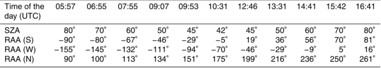
Simulations are carried out for all relevant combinations of viewing directions, SZA

and RAA (for SZA≤80◦). The diurnal cycle is described by 11 pairs of SZA and RAA,

respectively (see Table 1).

First, O₄ dAMF_α are calculated for all combinations of profile parameters shown in

Table 2. In total 250 000 O₄dAMF_α are calculated. In the next step, trace gas dSCD_α

10

are calculated for all combinations of profile parameters for the trace gas profiles and

the aerosol profiles (see Table 2). Accordingly, the number of trace gas dSCD_α

simu-lations is much larger (about 40 million) than the simusimu-lations of O₄dAMF_α. To reduce

the computational e_ffort, two simplifications were applied. First, it is assumed that the

dAMF_α for NO₂and HCHO_α do not depend on the respective VCDs. Except for very

15

high NO₂VCDs, this assumption is well fulfilled: for HCHO the respective error is

neg-ligible; for NO₂ VCDs<1×1017molec cm−2 the error is <5 % and can be neglected

compared to other uncertainties. Second, and related to the first point, HCHO and

NO₂ “total” tropospheric dAMF_α are not calculated directly. Instead, height-resolved

so called box air mass factors are determined, from which the total dAMF_α are

calcu-20

lated by the average of the box air mass factors, weighted with the respective (relative) height profile:

dAMF_α,_total₌

P

z

BoxdAMF_α(zi)·c(zi)·∆zi

P

z c

(zi)·∆zi

(14)

Here BoxdAMF_α(zi) indicates the differential box air mass factor, c(zi) the trace gas

concentration and∆z_i the height for the layer atz_i. dAMF_α are calculated for discrete

25

(20)

AMTD

4, 3891–3964, 2011

from MAX-DOAS

T. Wagner et al.

Title Page

Tables Figures

◭ ◮

Back Close

Full Screen / Esc

Discussion

P

a

per

|

Dis

cussion

P

a

per

|

Discussion

P

a

per

|

Discussio

n

P

a

per

|

stored in look-up tables (LUT). For a given measurement sequence, the LUT is first reduced corresponding to the actual SZA and RAA of the measurement by linear in-terpolation. The remaining LUT is used as forward model, to which the measurements are fitted.

After the aerosol profile parameters are determined as outlined above, the trace gas 5

profile parameters are retrieved taking into account the aerosol parameters retrieved in the first step. Note that the shape parameters and layer heights for the aerosol and trace gas profiles are retrieved independently.

3.3 Error estimation

Several error sources contribute to the total uncertainty of the profile inversion results. 10

Systematic errors are caused by errors of the spectroscopic data (e.g. uncertainties of the absorption cross sections and their spectral calibration) or deviations of the assumed optical properties of the aerosols used in the radiative transfer simulations (Sects. 3.2). Systematic errors might also be caused by other limitations of the forward

model, i.e. its inability to correctly describe cloud e_ffects or the real 3-dimensional trace

15

gas and aerosol distributions. These and other systematic errors are di_fficult to identify

and quantify. Here it is essential to compare the MAX-DOAS results with independent data sets (see Sects. 5.2 and 5.3).

Random errors are caused e.g. by the limited signal to noise ratio of the DOAS analy-sis and by spatio-temporal fluctuations of the trace gas and aerosol distributions (atmo-20

spheric noise). One e_ffect of random errors is that they cause deviations between the

individual measurements of an elevation sequence and their respective forward model results. While the forward model usually shows a smooth dependence on the elevation angle, the measurements often show additional fluctuations related to measurement or

atmospheric noise. The respective deviations are quantified by theχ2(sum of squares

25

of individual differences) between the measurements and the forward model. In the

following, retrieval results with large deviations between measurements and forward

(21)

AMTD

4, 3891–3964, 2011

from MAX-DOAS

T. Wagner et al.

Title Page

Tables Figures

◭ ◮

Back Close

Full Screen / Esc

Discussion

P

a

per

|

Dis

cussion

P

a

per

|

Discussion

P

a

per

|

Discussio

n

P

a

per

|

In addition to the χ2 between measurements and forward model, inversion errors

can also be quantified from the fit process itself (see also Li et al., 2010) taking into ac-count the sensitivity of the measured quantities with respect to variations of the profile parameters. Errors determined in this way in this study are representative for a con-fidence interval of 95 %. We found that the errors determined in this way are largely 5

proportional to the χ2, which indicates that they typically represent random errors of

the spectral retrieval and/or “atmospheric noise”.

From a linear fit of these errors versus the corresponding values of the profile pa-rameters, the typical relative errors are determined. To this regression line, a constant value is subsequently added to assure that for the smallest retrieved values the linear 10

parameterisation still matches the respective uncertainties. Thus this error estimate

represents an upper limit. The error parameterisations for the di_fferent retrieved

quan-tities are summarised in Table 3; they were used for the correlation analyses presented in Sect. 5.2. Also shown in Table 3 are the mean relative errors. They range from about

9 % for the NO₂mixing ratio to 71 % for the aerosol layer height.

15

3.4 Aerosol inversion

In the first step of the profile inversion, the aerosol extinction profile is determined

from the measured O₄DAMF (Eq. 2). Since MAX-DOAS spectra are analysed against

a fixed Fraunhofer reference spectrum (see Sect. 2.3), the retrieved O₄DAMF contain

not only the difference compared to the zenith spectrum of the same elevation

se-20

quence (as needed for the inversion), but also a SZA dependent offset. To remove this

o_ffset, the O₄DAMF for the 90◦elevation spectrum of the selected elevation sequence

is subtracted from the O₄DAMF for all other (slant) elevation angles of this sequence

to yield the respective dAMF_α.

In this study only two profile parameters (AOD and layer heightL) are varied during

25

(22)

AMTD

4, 3891–3964, 2011

from MAX-DOAS

T. Wagner et al.

Title Page

Tables Figures

◭ ◮

Back Close

Full Screen / Esc

Discussion

P

a

per

|

Dis

cussion

P

a

per

|

Discussion

P

a

per

|

Discussio

n

P

a

per

|

a shape parameter ofS=1 was used (“box” profile). In addition, we also determined

aerosol profiles for shape parameters ofS=0.8 andS=1.1 (for elevated layers both

linear profiles and two-layer profiles are used as defined in Sect. 3.1.1).

Fit results for selected elevation sequences are shown in Fig. 3 (top). The measured

O₄ dAMF_α are shown as black dots, while the fitted values are displayed as coloured

5

lines. In both cases the measurements can be well described by the forward model.

Interestingly, similar agreement is found for the different assumed profile shape

pa-rameters, illustrating that the information content of our MAX-DOAS observation is not

su_fficient to discriminate these di_fferent profile shapes.

For both examples, quite different general dependencies of the O₄ dAMF_α on the

10

elevation angles are found. For the example on 15 September 2003 the O₄ dAMF_α

increase continuously with decreasing elevation angle, while on 19 September 2003

they decrease for elevation angles<18◦. The corresponding aerosol extinction profiles

are also shown in Fig. 3 (bottom). While for 15 September 2003 the retrieved

pro-files and AODs di_ffer substantially for the di_fferent assumed shape parameters, on 19

15

September 2003 the aerosol profile inversion yields much more similar profiles and al-most the same AODs. Fortunately, for al-most measurements, the retrieved AODs hardly depended on the assumed shape parameter.

The dependence on the assumed shape parameter for the 15 September 2003 in-dicates a fundamental problem for the retrieval of the AOD in cases when the shape 20

parameter itself cannot be unambiguously retrieved in the inversion procedure. Similar results are found for other observations on 15 September 2003 (see Fig. 4 left) and also appeared for the observations of the two other telescopes (north and west direction, not shown). This indicates that the instability of the profile inversion is not an artifact for a single azimuth viewing direction, but is probably related to the specific properties 25

of the aerosol profile on that day. Instabilities for the AOD retrieval from MAX-DOAS observations were also reported by Li et al. (2010).

In Fig. 4 the retrieved layer heights and extinction coefficients for both days are also

(23)

AMTD

4, 3891–3964, 2011

from MAX-DOAS

T. Wagner et al.

Title Page

Tables Figures

◭ ◮

Back Close

Full Screen / Esc

Discussion

P

a

per

|

Dis

cussion

P

a

per

|

Discussion

P

a

per

|

Discussio

n

P

a

per

|

S≤1 or for the linear profile withS=1.1 are closely correlated to similar rapid changes

of the layer heightL(Fig. 4 middle). As a consequence the aerosol extinction (Eqs. 5,

8, 10) is much less dependent on the profile shape than the AOD (bottom panel of Fig. 4). Also the uncertainties of the retrieved aerosol extinction are much smaller than those of the AODs or layer heights.

5

On 19 September 2003 a di_fferent behaviour compared to 15 September is found:

the extinction coefficient depends more strongly on the assumed profile shape than the

AOD (see Fig. 4 right). Also the uncertainties of the aerosol extinction is much larger indicating that on that day a two-layer profile with shape parameter of 1.1 might not be a good choice for the determination of the aerosol extinction. Here it should be noted, 10

that the aerosol extinction determined for the two layer profile with zero values at the surface can by definition not be representative for the actual aerosol extinction at the surface (the data in Fig. 4 is shown again in the Supplement (Fig. S1), but with the uncertainties displayed for the retrieval assuming a box profile).

We investigated possible reasons for the instabilities of the aerosol profile inversion 15

and the dependence of the AOD on the profile shape. One hypothesis is that on 15 September 2003 an elevated aerosol layer might have been present. An indication for

this hypothesis is found in the results for shape parameters S >1. If profiles for an

elevated aerosol layer are used (either a linear profile or a two-layer profile), the diurnal variation of the AOD shows a much smoother behaviour. The most consistent temporal 20

variation is found for a two-layer parameterisation (assuming a layer with zero aerosol extinction at the surface).

We further tested our hypothesis of an elevated layer by performing radiative transfer

simulations for di_fferent assumed aerosol extinction profiles (see Fig. 5). It turned out

that for the elevation angles used in this study (≥3◦, indicated by the black arrows), the

25

simulations for a two-layer profile with shape parameter of 1.1 (andL=1, AOD=0.3)

can be well reproduced by the simulations for a box-profile (shape parameter of 1),

but with larger values forL and AOD (4 km and 1, respectively). Also the simulations

(24)

AMTD

4, 3891–3964, 2011

from MAX-DOAS

T. Wagner et al.

Title Page

Tables Figures

◭ ◮

Back Close

Full Screen / Esc

Discussion

P

a

per

|

Dis

cussion

P

a

per

|

Discussion

P

a

per

|

Discussio

n

P

a

per

|

the hypothesis that in the presence of elevated aerosol layers, no unambiguous profile inversion might be possible for the elevation angles used in this study.

The ambiguity demonstrated in Fig. 5 can explain the observations on 15 Septem-ber 2003 (Fig. 4 left), for which increased AOD are often found with simultaneously enhanced layer height. They also indicate that if additional viewing angles at low el-5

evation were included in the MAX-DOAS observations, the ambiguity of the profile

retrieval could be effectively reduced.

It should be noted that a profile with zero aerosol extinction at the surface is probably not very reasonable close to strong emission sources like for our measurements (see discussion in Sect. 3.1.1). Nevertheless, the smooth diurnal variation found for this 10

profile parameterisation indicates that strong vertical gradients of the aerosol extinction probably exist close to the surface, which are better described by the two-layer profile than by the other profile parameterisations.

To deal with the problem of underdetermination of the aerosol profile, we chose a pragmatic solution by simply using a shape parameter of 1.1 (two layer profile) for 15

the determination of the AOD. By this choice, stable results for the AOD are obtained for all days (see Fig. 4 left). But of course, this choice has also disadvantages: The

retrieved AOD is often smaller than for shape parametersS≤1 (see Fig. 4 right), but

this underestimation is usually small (less than 10 %). Another disadvantage is that the

retrieved layer height for a shape parameter ofS=1.1 is systematically lower (typically

20

by a factor of about 2) than for a shape parameter of 1 (Fig. 4, middle). There is

proba-bly no simple explanation for this finding, but the fact thatL₁_.₁is systematically smaller

thanL1.0 is consistent with the results of the radiative transfer simulations presented

in Fig. 5. Note that the results for the aerosol layer height presented in the following sections were retrieved for a shape parameter of 1.1, and were subsequentially multi-25

(25)

AMTD

4, 3891–3964, 2011

from MAX-DOAS

T. Wagner et al.

Title Page

Tables Figures

◭ ◮

Back Close

Full Screen / Esc

Discussion

P

a

per

|

Dis

cussion

P

a

per

|

Discussion

P

a

per

|

Discussio

n

P

a

per

|

Also, for shape parameters S <1 systematically lower layer heights are retrieved

than forS=1. This has to be expected, because for theseS-values a substantial part

of the aerosol load is located above the “aerosol layer”.

While for our measurements, an aerosol profile withS=1.1 is probably a good

(prag-matic) choice for the retrieval of the AOD and layer height, it is not necessarily a good 5

choice for other retrieved quantities. For example, as shown in Fig. 4, for shape

param-etersS≤1 the retrieval of the aerosol extinction leads to much more consistent results.

As will be shown below, the results of the trace gas inversions (especially for the trace gas VCD and layer height) are also more realistic and consistent, if shape parameters

S≤1 for the aerosol profile inversion are chosen.

10

3.5 Trace gas inversion (NO2and HCHO)

The inversion of the trace gas profiles (second step) is performed in a similar way to

the aerosol inversion. First the DSCDs for the 90◦elevation angles are subtracted from

the DSCDs of the lower elevation angles of the same sequence to yield the respective

dSCD_α. In the next step the trace gas dSCD_αare divided by the dSCD_αfor an elevation

15

angleα=10◦ of the same elevation sequence (in principle any other elevation angle

could be used as well). This normalisation is performed to simplify the fitting process

of the trace gas inversion. In contrast to the aerosol inversion, where the O₄ DAMF

depend not only on the relative profile shape but also on the absolute value of the AOD,

the dAMF_αfor NO₂and HCHO depend only on the relative profile shape, because their

20

atmospheric absorptions are weak (OD typically<0.1). Thus, the profile inversion for

NO₂and HCHO can be reduced to the determination of the relative profile shapes (also

see Sinreich et al., 2005).

Before the fit to the normalised trace gas dSCD_α, a similar normalisation of the

dAMF_α of the forward model is applied. From the fit between the measurements and

25

the forward model, the (relative) profile shape (layer height, and shape parameter) and

the corresponding dAMF_α are obtained. From these dAMF_α and the measured trace

(26)

AMTD

4, 3891–3964, 2011

from MAX-DOAS

T. Wagner et al.

Title Page

Tables Figures

◭ ◮

Back Close

Full Screen / Esc

Discussion

P

a

per

|

Dis

cussion

P

a

per

|

Discussion

P

a

per

|

Discussio

n

P

a

per

|

VCD_α=dSCDα

dAMF_α (15)

Finally, the average of the VCDs for the di_fferent elevation sequences is calculated.

From the VCD, the layer height, and the shape parameter the average trace gas con-centration or mixing ratio is calculated according to Eqs. (6), (7), (9), and (11). Like the aerosol inversion, in some cases the trace gas inversion has no stable convergence, 5

and thus, the shape parameterS, is prescribed. Thus only the layer heightLand the

VCD were determined independently by the fit.

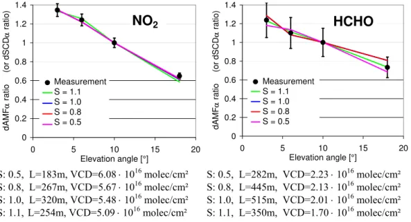
In Fig. 6 exemplary fit results of the forward model to the measured (normalised)

dSCD_α of NO₂ and HCHO are shown. Like the aerosol inversion, similar agreement

for the different shape parameters is found. The VCDs retrieved for shape

parame-10

ters≤1 show rather good agreement, but for shape parameters>1 (elevated layers),

systematically lower VCDs are obtained. However, in contrast to the aerosol inversion, the results of the trace gas inversions did not show instabilities like those in Fig. 4 (left

column). Thus in the following, only trace gas results for shape parameters ≤1 are

presented. The better convergence of the trace gas VCDs (compared to the AOD) is 15

probably caused by fact that enhanced concentrations of NO₂ and HCHO are usually

confined to the lowest atmospheric layers, while the atmospheric scale height of O₄is

about 4 km.

In Fig. 7 the diurnal variations of the retrieved trace gas results (VCD, layer height and mixing ratio) are presented for 19 September 2003. For comparison, the mixing 20

ratios of the independent measurements (LP-DOAS and Hantzsch) are also shown. In

general, the HCHO layers (and their uncertainties) are higher than those of NO₂.

The trace gas VCDs from the profile inversion are compared to the respective VCDs calculated by the so called geometric approximation (Andreas Richter, personal com-munication, 2006; Brinksma et al., 2008). In this study we used the measurements at 25

(27)

AMTD

4, 3891–3964, 2011

from MAX-DOAS

T. Wagner et al.

Title Page

Tables Figures

◭ ◮

Back Close

Full Screen / Esc

Discussion

P

a

per

|

Dis

cussion

P

a

per

|

Discussion

P

a

per

|

Discussio

n

P

a

per

|

VCD_geo=dSCD18◦

dAMF₁₈◦ =

dSCD₁₈◦

1/sin(18◦)−1 (16)

While the trace gas VCDs from the profile inversions assuming different shape

param-eters show very good agreement, the geometric VCDs are mostly smaller than the VCDs from the profile inversions (especially for periods with high trace gas VCDs).

These di_fferences are most probably caused by the neglect of scattering processes in

5

the calculation of the geometric VCD. The systematic deviations between the geomet-ric VCD and the VCDs from the profile inversion are further investigated in Sect. 5.2.4. As pointed out before, the results of the aerosol inversion are used as input for the trace gas profile inversion. Thus the question arises, which aerosol shape parameter

S_aershould be used in the first step of the trace gas retrievals. To answer this question

10

we compared trace gas results for di_fferent assumed aerosol shape parameters S_aer

(for simplicity, the shape parameter for the trace gas inversionS_tracegas was set to 1).

The results are presented in Fig. 8. While the trace gas mixing ratios are only slightly

a_ffected by di_fferent choices ofS_aer, the trace gas VCDs and layer heights for di_fferent

S_aershow large differences. Especially forS_aer>1 they deviate systematically from the

15

results forSaer≤1. The reason for this finding is not clear, but is probably related to

the fact that for aerosol shape parametersS_aer>1 the aerosol extinction close to the

ground is systematically underestimated. This is the layer where usually the highest trace gas concentrations occur. Fortunately, the trace gas mixing ratios depend little on the assumed aerosol shape parameter.

20

4 Influence of clouds on MAX-DOAS observations

Like aerosols, clouds also strongly a_ffect the atmospheric radiative transfer and can

have a large e_ffect on MAX-DOAS observations and the profile retrievals. Thus, the

profile inversion for measurements at cloudy conditions is probably strongly influenced

by clouds. In this section the e_ffects of clouds on MAX-DOAS measurements are