Geosci. Model Dev., 6, 161–177, 2013 www.geosci-model-dev.net/6/161/2013/ doi:10.5194/gmd-6-161-2013
© Author(s) 2013. CC Attribution 3.0 License.
Geoscientiic
Model Development
Open Access
Geoscientiic
Implementation of the Fast-JX Photolysis scheme (v6.4) into the
UKCA component of the MetUM chemistry-climate model (v7.3)
P. J. Telford1,2, N. L. Abraham1,2, A. T. Archibald1,2, P. Braesicke1,2, M. Dalvi3, O. Morgenstern4, F. M. O’Connor3,
N. A. D. Richards5, and J. A. Pyle1,2
1NCAS Climate, University of Cambridge, Cambridge CB2 1EW, UK
2Centre for Atmospheric Science, Department of Chemistry, University of Cambridge, Cambridge CB2 1EW, UK 3Met Office Hadley Centre, Exeter, UK
4National Institute of Water and Atmospheric Research, Lauder, New Zealand
5Institute for Climate and Atmospheric Science, School of Earth and Environment, University of Leeds, UK
Correspondence to:P. J. Telford ([email protected])
Received: 3 October 2012 – Published in Geosci. Model Dev. Discuss.: 17 October 2012 Revised: 10 January 2013 – Accepted: 15 January 2013 – Published: 7 February 2013
Abstract.Atmospheric chemistry is driven by photolytic
re-actions, making their modelling a crucial component of at-mospheric models. We describe the implementation and val-idation of Fast-JX, a state of the art model of interactive pho-tolysis, into the MetUM chemistry-climate model. This al-lows for interactive photolysis rates to be calculated in the troposphere and augments the calculation of the rates in the stratosphere by accounting for clouds and aerosols in addi-tion to ozone. In order to demonstrate the effectiveness of this new photolysis scheme we employ new methods of validat-ing the model, includvalidat-ing techniques for samplvalidat-ing the model to compare to flight track and satellite data.
1 Introduction
In the recent past efficient comprehensive photolysis schemes have been developed that are fast enough to be run within global, three dimensional models, allowing a more in-teractive treatment of photolysis rates in composition mod-elling (Wild et al., 2000; Tie et al., 2003). These have been implemented into a range of global, three dimensional mod-els (see for instance Liu et al., 2006; Voulgarakis et al., 2009) and have been demonstrated to provide an improved descrip-tion of atmospheric composidescrip-tion, especially in regions with large variability in optical depths. The optical depth of the at-mosphere is composed of several constituents, including the air itself, a phenomenon known as Rayleigh scattering,
oxy-gen, ozone, clouds, and aerosols (see, for instance, Wild et al. (2000) for more details) .
The UKCA module is a component of the UK Met Of-fice’s Unified Model (MetUM). A number of model config-urations have been established and tested; one with strato-spheric chemistry (Morgenstern et al., 2009), one with tro-pospheric chemistry (O’Connor et al., 2009; O’Connor et al., 2013; Telford et al., 2010) and one with the GLOMAP-mode aerosol scheme (Mann et al., 2010). There are also whole atmosphere chemistry schemes that have been de-veloped from the tropospheric and stratospheric chemistries (Archibald et al., 2012; Morgenstern et al., 2012). We de-scribe the addition of the Fast-JX photolysis code into the MetUM framework and evaluate it against a range of obser-vations.
the performance of the stratospheric model by comparing to-tal ozone column and ozone profiles to observations.
2 Model description
The UKCA chemistry module is part of the Met Office’s Uni-fied Model (MetUM). We employ a version of the model based on the HadGEM3 configuration (Hewitt et al., 2011), but with the following configuration:
– a horizontal resolution of 3.75◦×2.5◦in longitude and latitude.
– 60 hybrid height levels in the vertical, from the surface up to a height of 84 km.
A time series of sea surface temperatures and sea ice cov-erage are prescribed from the HadISST dataset (Rayner et al., 2003).
2.1 Nudging
The technique of nudging is used to reproduce the atmo-spheric conditions over the period studied. The nudging is applied from 3 to 45 km with a relaxation timescale of 6 h (Telford et al., 2008). For the first time we nudge to the Interim reanalysis data (Dee et al., 2011) instead of the ERA-40 reanalyses. ERA-Interim are the latest reanalysis products from the ECMWF with the following changes from the ERA-40 reanalysis: higher horizontal resolution, 4D-var data as-similation, new humidity analyses, improved model physics, and a different period of coverage (1979–2012 compared to 1957–2002 in ERA-40).
2.2 Tropospheric chemistry
The tropospheric version of the model employs a medium-sized chemistry scheme that simulates the Ox, HOxand NOx
chemical cycles and the oxidation of CO, ethane, propane, and isoprene (Telford et al., 2010). The Mainz isoprene mechanism (P¨oschl et al., 2000) is used to parameterise iso-prene oxidation. In total the model has 168 chemical reac-tions and 56 chemical tracers. We also add the additional reaction between HO2 and NO using the rates and yields
of Butkovskaya et al. (2007) and hydrolysis of N2O5
(Mor-genstern et al., 2009). Concentrations of ozone and NOy
are overwritten above 30 hPa. The upper boundary condi-tion for NOyare taken from the Cambridge 2-D model (Law
and Pyle, 1993a,b). The upper boundary conditions for O3
are taken from the Rosenlof climatology (Dall’Amico et al., 2010), with the model values being overwritten above the up-per boundary. Methane is fixed to 1.76 ppm throughout the atmosphere. Dry deposition and wet deposition are parame-terised using the approaches of Giannakopoulos et al. (1999). Seven chemical species (nitrogen oxide (NO), carbon monoxide (CO), formaldehyde (HCHO), ethane, propane,
acetaldehyde and acetone ((CH3)2CO)) are emitted in the
manner of Zeng and Pyle (2003). Isoprene (C5H8) emissions
are included in a similar manner, though with a diurnal cy-cle as in Young (2007). The emissions are taken from a sum of anthropogenic and natural emissions, with anthropogenic and biomass burning emissions taken from Lamarque et al. (2010) using data for the year 2000. We also lump the emis-sions of ethene and ethyne with ethane, and propene with propane. Aircraft emissions of NO are taken from Eyers et al. (2004). We also include biogenic emissions of CO, Me2CO
and C5H8and emissions of NO from natural soil emissions
and lightning. The biogenic emissions are distributed accord-ing to Guenther et al. (1995) and total 40 Tg yr−1of CO from
the oceans and 45 Tg yr−1of CO, 40 Tg yr−1of Me
2CO and
570 Tg yr−1of C
5H8from the land. We include, on average,
5 Tg yr−1of N from lightning emissions, distributed
accord-ing to the parameterisation of Price and Rind (1994). Finally we include 5.6 Tg yr−1of N from natural soil emissions
dis-tributed according to the empirical model of Yienger and Levy II (1995). The model uses the aerosol model of Bel-louin et al. (2007) using emissions from 2000.
2.3 Stratospheric chemistry
The stratospheric version of the model has a comprehen-sive stratospheric chemistry, including chlorine and bromine chemistry, heterogeneous processes on polar stratospheric clouds (PSCs), and liquid sulphate aerosols as well as a sim-plified tropospheric chemistry (Morgenstern et al., 2009). More detailed descriptions of the stratospheric version of the chemistry can be found in Morgenstern et al. (2009).
There are a few differences between the stratospheric model used in this study and that in Morgenstern et al. (2009). The base version of the climate model has been up-dated to HadGEM3 from HadGEM1a. In addition, N2O is
now transported completely separately from the other odd nitrogen species and the reaction N2O+O(1D) has been
up-dated with rates from a more recent JPL assessment (Sander et al., 2006).
2.4 Offline photolysis schemes
In earlier versions of the model, photolysis rates were de-termined from rates calculated offline under average con-ditions, tabulated and interpolated for use online. There were two schemes, one for use in the troposphere, and one for use in the stratosphere. The tropospheric configuration of the chemistry model exclusively used the tropospheric photolysis scheme. The stratospheric configuration of the chemistry model used the tropospheric photolysis scheme below 300 hPa, the stratospheric photolysis scheme above 200 hPa with a linear transition between the two schemes from 200 hPa and 300 hPa.
a zonally averaged offline distribution (Law et al., 1998). The photolysis rates depended only on latitude, local so-lar time, month of the year and pressure. The stratospheric scheme was based on the look up table approach of Lary and Pyle (1991), with some updated cross-section measure-ments (Morgenstern et al., 2009). The rates in the strato-spheric scheme responded to changes in the overhead ozone column using a simple scaling.
Apart from a simple scaling to account for changes in stratospheric ozone in the stratospheric scheme, these schemes did not respond to changes in optical depth, rely-ing instead on average conditions for particular latitudes and altitudes. This precluded us from looking at a complete set of feedbacks caused by variations in the optical depth (from e.g. clouds, aerosols) onto atmospheric composition, limit-ing our ability to simulate the atmosphere. The addition of a more complete interactive photolysis scheme allows us to overcome this hurdle.
2.5 Fast-J interactive photolysis schemes
Recently, interactive photolysis schemes have been devel-oped that are fast enough to be incorporated into global mod-els. The original Fast-J scheme was developed for tropo-spheric photochemistry (Wild et al., 2000). It arranged light from wavelengths between 289 to 850 nm into seven discrete bins. A further development, Fast-J2, extended the scheme into the stratosphere (Bian and Prather, 2002) by adding 11 wavelength bins from 177–290 nm. To speed up the code, the Rayleigh scattering for the additional wavelengths was treated as pseudo absorption. In the absence of this scatter-ing, Fast-J2 fails to reproduce stratospheric photolysis rates at low solar zenith angles or at dusk, yielding problems in the high latitude winter stratosphere (Morgenstern et al., 2009) and has difficulties in describing the effects of high aerosol loadings. Fast-JX builds on these two schemes, providing the full scattering calculation for all 18 wavelength bins (Neu et al., 2007). It also has several other improvements, most notably a more efficient way of introducing extra levels for very optically dense clouds. It is the implementation of this code1into the MetUM model that we describe.
3 Technical implementation
We take the Fast-JX code from the Fast-JX website2, here-after referred to as Prather et al. (2010). Given the optical depth from absorbing and scattering species, this code deter-mines how many photons of each wavelength are absorbed and scattered as light passes through the atmosphere.
This is done using the “plane parallel assumption” which assumes that, for a grid box, the horizontal properties are constant and radiative transfer properties only depend on
1Version 6.4
2http://www.ess.uci.edu/∼prather/fastJX.html (version 6.4)
the vertical coordinate. Radiative fluxes between horizontally adjacent grid boxes is also neglected. The calculation of the radiative properties thus divides into a series of columns. The path of the radiation is traced through this column, being scattered or absorbed according to the contents of the grid box. The amount of scattering and absorption depends on the optical depth of the different scatterers in the grid box.
The photolysis rates (“j” rates) for each reaction are de-termined from the wavelength bin-resolved flux in each grid box and the cross section of each species in each wave-length bin. These cross sections are evaluated from exper-imental measurements of the photolysis rates as described in Sect. 3.2 and, apart from O3, are actually a product of
the absorption cross section and quantum yield for a partic-ular reaction. In ozone the total absorption cross section and quantum yields are calculated separately. Because Fast-JX still does not provide photolysis rates for wavelengths below 177 nm, which are important for some reactions in the up-per stratosphere and mesosphere we evaluate the cross sec-tions for these wavelengths using the original offline scheme from Lary and Pyle (1991) and add them to the Fast-JX reac-tion rates. For speed this extra calculareac-tion is only performed above 20 Pa, as below this level the flux of these high energy photons is negligible.
3.1 Calculation of optical depth
The optical depth (τ) is determined as the sum of the opti-cal depth of ice water clouds (τw), liquid water clouds (τi), aerosols, ozone and oxygen and Rayleigh scattering.
The optical depth of liquid water clouds is calculated using the parameterisation of Slingo (1989),
τw=LWP
ai+
bi reff
. (1)
Here LWP is the liquid water path of the cloud, ai and
bi are parameters and reff is the effective radius of the
water droplets. The parameters, which are taken to be
−8.9 m2kg−1and 1.67×10³m3kg−1, are updated from Ed-wards and Slingo (1996). The effective radius is assumed to be 6 µm over land and 12 µm over water.
The optical depth of ice water clouds is calculated using the non spherical parameterisation of Edwards et al. (2007),
τi=IWP ci+ di deff
+ ei deff2
!
. (2)
Here IWP is the ice water path of the cloud,ci,di and ei
are parameters updated to account for the different spec-tral bands anddeff is the effective diameter of the ice parti-cles. The values ofci,diandeiare−2.189 m2kg−1, 3.311×
10−3m kg−1and 3.611×10⁻¹²kg−1, respectively. The
ef-fective diameter is taken to be 100 µm.
means of doing it. We account for this effect using the simple approach of Briegleb (1992) where the optical depth is mod-ified by the factorf3/2, wheref is the fraction of each grid box area covered by clouds. This has been demonstrated by Feng et al. (2004) to produce a computationally cheap rep-resentation of the effects of overlapping cloud layers being used extensively in global models (Liu et al., 2006; Voulgar-akis et al., 2009).
The only aerosol accounted for at present is sulphate, which is taken from the models’ own fields. The effect of hygroscopic growth on particle size and optical depth is pa-rameterised using the approach of Fitzgerald (1975) as used by Bellouin et al. (2007).
The ozone, oxygen and Rayleigh scattering optical depths are calculated from the molecular columns (mol cm−2) of
ozone, oxygen and total air mass, multiplied by the cross sec-tions for O3, O2and for Rayleigh scattering. The molecular
column for raleigh scattering is calculated from the density in a grid box, the column for O2is calculated from the
den-sity multiplied by the mixing ratio of O2in the atmosphere,
which is assumed to be constant (0.2095). The ozone column is calculated from the density multiplied by the mixing ratio of O3in each grid cell.
All optical depths are determined at 600 nm and then scaled for the different wavelength bins. For the purposes of determining the addition of extra levels in the presence of high optical depths, only the cloud optical depth is used.
3.2 Calculation of cross sections
The cross sections are based on v6.4 of the file available from the Fast-JX website (Prather et al., 2010). This data set is a combination from the JPL14 assessment (Sander et al., 2003) with the addition of IUPAC data for NO2 and VOC
photolysis rates and of other sundry additions such as the acetone photolysis of Blitz et al. (2004) and the infrared pho-tolysis of HO2NO2of Jim´enez et al. (2005). We have updated
these cross sections to include data from JPL15 assessment (Sander et al., 2006), with the most notable changes includ-ing updates for N2O5and OClO photolysis. We summarise
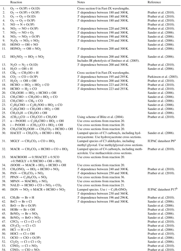
all reactions described, noting whether they are utilised by the stratospheric or tropospheric chemistry, in Table 4.
4 Methodology
To test the performance of the model we carry out a series of tests. The first of these is to investigate how the standalone photolysis code performs under idealised conditions. To do this we employ the scenarios devised for the PHOTOCOMP photolysis study as part of the CCMVal chemistry-climate model intercomparison (Chipperfield et al., 2010).
We then proceed to investigate how the MetUM model with the Fast-JX photolysis included performs. To do this we perform a run with the tropospheric chemistry version
of the model, from 2004 to 2008 and compare two different sets of observations, including data from the INTEX cam-paign and the TES satellite instrument. To enable us to make more direct comparisons we run the model in “nudged mode” (Telford et al., 2008). This constrains the model to meteoro-logical observations, making comparisons with data over our chosen years more meaningful.
The first brief check we make is to ensure that nudging with the ERA-Interim dataset is as successful as nudging with the ERA-40 dataset. We do this by comparing biases, correlations and root mean square differences between the nudged model and analyses as used by Telford et al. (2008). We then proceed to compare photolysis rates with observa-tions from the INTEX-NA campaign, sampling the model at the time and location of the measurements. We make a quan-titative assessment of the offline and interactive photolysis schemes by comparing biases, correlations and root mean square differences (RMSD) between the model and the ob-servations.
We then study the effects these changes in photolysis rates have on atmospheric composition, focusing on ozone and carbon monoxide. Our principal comparisons are with observations from the TES satellite instrument, compar-ing both the distributions of CO and O3 and their
cor-relation. We sample the model in a similar manner to Rodgers and Connor (2003), taking measurements at the ap-propriate time and location at the satellite and applying the instrument’s averaging kernels to make comparisons more meaningful. To understand the changes in the chemical species distributions we also study the ozone budgets and changes in OH.
Finally, we briefly examine results from a stratospheric simulation, comparing the total ozone column with obser-vations. For this run we do not use nudging in order to al-low feedbacks from chemistry to dynamics to influence the model.
5 Model results
5.1 Idealised comparison
We first check the photolysis rates of NO, O2and O33
un-der idealised conditions using the three assessed scenarios from the PHOTOCOMP assessment of the CCMVal model intercomparison (see Sect. 6.3.1 in Chipperfield et al., 2010). These employed idealised atmospheric conditions to allow systematic comparisons between the photolysis in different models. The three scenarios used clear sky conditions with a solar zenith angle of 15◦, 84◦and averaged over a day be-tween 84◦and 96◦.
We compare photolysis rates as a function of altitude in a series of idealised atmospheric profiles constructed for a multi-model comparison study. The photolysis rates for
3This is the total O
log (j-NO)
0.1
1
10
100
1000
]a
Ph[
er
uss
er
P
-10-9 -8 7- -6 -5 -4
0.1
1
10
100
1000
]a
Ph[
er
uss
er
P
log(j-O2)
-14-13-12-11-10-9 -8 -7-6 -5 -4 -3 -2 -1 0.1
1
10
100
1000
]a
Ph[
er
uss
er
P
log(j-O3t)
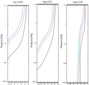
Fig. 1.Photolysis rates for the CCMVal photolysis assessment
sce-narios for NO (left), O2 (centre) and O3 (right). The three lines correspond to a solar zenith angle of 15◦(black), 84◦(pink) and averaged over a day between 84◦and 96◦(blue). This figure can be compared to Fig. 6.1 in Chipperfield et al. (2010).
NO, O2and O3are shown in Fig. 1, which can be compared
to Fig. 6.1 in Chipperfield et al. (2010).
The O3photolysis rates look similar to the PHOTOCOMP
average, reducing from around 10−2s−1 at 0.1 hPa to
be-tween 10−4–10−3s−1near the surface, depending on the
so-lar zenith angle. Simiso-larly, the O2photolysis rates look
sim-ilar to the PHOTOCOMP average, reducing from around 10−9s−1 at 0.1 hPa to below 10−14s−1 between 20 and 200 hPa depending on the solar zenith angle. The NO photol-ysis rates are the exception, being highly biased throughout the atmosphere. At the top of the atmosphere the photolysis rates are around 10−5s−1in contrast to the PHOTOCOMP
average, which is nearer to 10−6s−1. This is consistent with
the models that employ Fast-JX in the PHOTOCOMP study, which see good agreement with the multi-model mean pho-tolysis rates for O2and O3, but report a high bias in the case
of NO. This discrepancy has been linked to factors such as a neglect of NO absorption in the calculation of the optical depth, leading to an overestimate of the modelled cross sec-tion. Indeed in the latest versions of Fast-JX the NO photol-ysis has been scaled by a factor of 0.6 to account for these factors.
Given the general successful performance under idealised conditions, we move on to studying the effects of the photol-ysis code within the wider chemistry climate model.
5.2 Validation of nudged tropospheric MetUM run
After demonstrating that the standalone photolysis scheme works well under idealised conditions we test the perfor-mance of the scheme within a MetUM model run.
Table 1.Quantitative assessment of model performance in October
2005 with ERA-Interim nudging using the statistical assessments of Telford et al. (2008) for potential temperature (θ) and zonal wind (u). This calculates the model mean on four representative model levels and determines the root mean squared error (RMSE) and cor-relations over time (TC) and space (SC) with respect to the ERA-Interim analyses on these same levels.
Level Mean and Bias RMSE TC SC
θ
6 285.3+0.5 K 2.7 K 0.75 0.98
16 306.8+0.1 K 0.5 K 0.97 1.00
29 414.9+0.1 K 0.6 K 0.99 1.00
35 608.5+0.2 K 1.0 K 0.98 1.00
u
6 4.19+0.01 m s−1 3.37 m s−1 0.79 0.91
16 7.40−0.01 m s−1 1.45 m s−1 0.96 0.99
29 13.52−0.13 m s−1 1.17 m s−1 0.97 1.00
35 16.19−0.22 m s−1 1.37 m s−1 0.97 1.00
5.2.1 Validation of nudging with ERA-Interim analyses
As this is the first time we have used ERA-Interim reanal-ysis data in the nudging we briefly re-evaluate the nudg-ing performance. To do this we use the simple statistical tests of Telford et al. (2008), calculating the bias, correla-tion and root mean square difference between the nudged model and the ERA-Interim data, which show how similar the nudged model is to the ERA-Interim analyses. These re-sults are shown in Table 1. The performance of the nudging is broadly similar to that when using ERA-40 (compare to Ta-ble 1 in Telford et al., 2008), with the most notaTa-ble difference being the reduction in the RMSE of potential temperature (θ) in the stratosphere. This could reflect improvements in the data assimilation in the stratosphere (Dee et al., 2011), or just changes in the underlying model. Although the RMSE for potential temperature decreases, a small bias in zonal wind is introduced, so it is not just unalloyed improvement. Even so, from these results, we conclude that the model nudged towards the ERA-Interim analyses can be used as a hindcast of the period 2004 to 2008. This is consistent with the re-sults of Kipling et al. (2013) who show that nudging towards ERA-Interim analyses was able to improve modeled aerosol properties.
5.2.2 Comparison of cloud optical depth
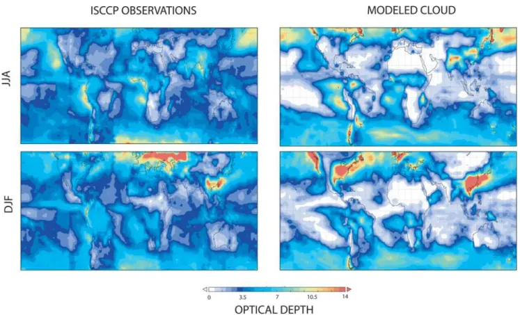
Fig. 2.Average cloud optical depth from ISCCP satellite data (left) and the UM (right). The top row contains a comparison for the Northern Hemisphere summer season and the bottom row for the winter season.
of several NOAA (the American National Oceanic Atmo-spheric Administration) satellites. The comparisons for De-cember, January and February 2005 and June to August 2005 are shown in Fig. 2.
The model is able to capture many of the features of the observations. For instance the storm tracks in the Northern Atlantic and Pacific oceans are well reproduced, as are the decks of stratus clouds off the coast of Peru. There are some discrepancies between the model and data, for instance the model underestimates the optical depth in the intertropical convergence zone (ITCZ). It also produces too large opti-cal depths over land in the winter, notably China, the Pa-cific coast of North America and the eastern USA in DJF and Chile in JJA, which may reflect an underestimate of the radii of the cloud particles in these locations at this time. Some of the other differences can be attributed to issues with the data, with errors introduced at high solar zenith angles, con-tamination from dust, and an underestimate of the amount of optically thick cloud (Marchand et al., 2010). For instance the discrepancy between the model and observations over the Sahara is likely a result of factors such as dust in the mea-surements rather than a deficiency in clouds in the model. However some of the discrepancies can be attributed to the simplified calculation of cloud optical depth and the limited resolution of the model. From the general good agreement we
conclude that the model is able to provide a reasonable de-scription of the cloud optical depth, with the agreement being at least as good as that in other models (see e.g. Voulgarakis et al., 2009).
5.2.3 Comparison of photolysis rates with INTEX
campaign data
0 100 200 300 400 500 Time (Minutes)
0.000e+00
6.250e
ï
05
1.250e
ï
04
jO(1D) (/s)
0
500
1000
Pressure [hP
a]
Pressure (hPa) UKCA (Climatological) UKCA (Interactive) INTEX
0 100 200 300 400 500
Time (Minutes)
0.00
0.01
0.02
0.03
0.04
jNO2 (/s)
0
500
1000
Pressure [hP
a]
Pressure (hPa) UKCA (Climatological) UKCA (Interactive) INTEX
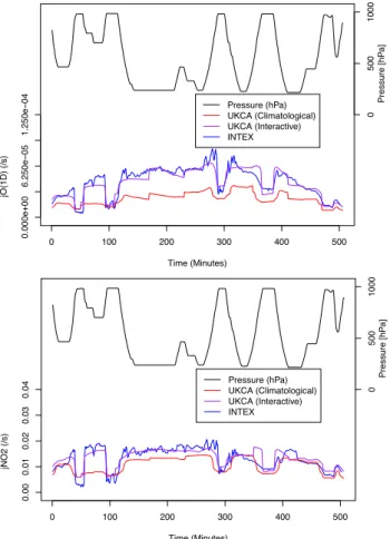
Fig. 3.Comparison of O3→O(1D)(top) and NO2(bottom)
pho-tolysis rates during the first flight (1 July 2004) in the INTEX-A campaign between observations and the model with offline and in-teractive photolysis rates.
to O’Connor et al. (2005) and employed by Kipling et al. (2013), interpolating the model to the pressure and coor-dinates where the measurements were made. As noted by O’Connor et al. (2005), the relatively low resolution that we use will prevent us from resolving small scale features in the observations. However we expect that we can produce the larger scale features relating to altitude, latitude and time of day. Figure 3 shows the O3and NO2photolysis rates from
the first flight of the INTEX-A campaign (1 July 2004) and in the MetUM model, with and without interactive photolysis rates.
The O3 photolysis rate is shown to be significantly
im-proved by the use of the interactive photolysis rates, with the low bias removed. The capture of the variability of the pho-tolysis rates is also improved, reflecting that the improved ability of the interactive photolysis rates to NO2 photolysis
rate is not as dramatic, though it can be seen that the in-teractive photolysis reduces a smaller bias and captures the variability better.
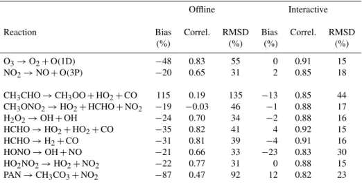
Figure 3 only shows one flight from the entire campaign. Although we chose this at random, selecting the first flight in the data, it is possible that the conditions might favour one photolysis scheme in particular. Therefore we calculate the bias, correlation, and root mean square difference (RMSD) between the modelled photolysis rates and the observed rates for all flights (1 July 2004 to 15 August 2004). The biases provide information on average rates. The correlations in-dicate the ability of the model to capture the variability in the photolysis. The RMSD combines information about av-erage agreement and variability. The biases, correlations and RMSD are given in Table 2 for the two rates shown in Fig. 3, along with selected other rates.
The tabulated results are in accord with Fig. 3, with the interactive photolysis having lower biases and higher corre-lations with the data than the offline photolysis. For several reactions, including O3photolysis, the discrepancy between
the offline photolysis and the data is considerably larger than the reported experimental uncertainty. For the interactive photolysis there are much smaller differences between the average model and observed values. Some of the reactions where there are differences between the model and the in-teractive photolysis and data, most notably HONO, are those where there have been updates to the reference cross sec-tions. In the case of HONO, the values (Sander et al., 2006) used in the interactive photolysis now incorporate additional measurements (Kenner and Stuhl, 1986; Stutz et al., 2000). This is relevant as the observed photolysis rates are not mea-sured directly, but are a product of the meamea-sured radiation multiplied by cross sections from Sander et al. (2003). So some of the discrepancy can be attributed to an improved un-derstanding of the experimental cross sections. Whilst some of the bias with the offline scheme can be attributed to the failure to update the photolysis rates using more recent mea-surements and a simple treatment of cloud optical depth, much can be attributed to an overestimation of the strato-spheric ozone column in the ozone climatology used to de-rive the offline photolysis rates.
By inspecting Fig. 3 we also see, as expected, that the global model, with either photolysis scheme, is not designed to describe small-scale variations. However the use of the interactive photolysis, rather than the offline scheme, does produce notable improvements. The correlation between the interactive photolysis and data is always greater than 0.8 and only greater than 0.8 for the photolysis rates of one species, HCHO, with the offline scheme. This can be explained by the fact that the photolysis rates are now sensitive to changes in cloud optical depth.
Table 2.Quantitative comparison between photolysis rates from INTEX data and modelled rates with interactive and offline photolysis using all flights (1 July 2004 to 15 August 2004).
Offline Interactive
Reaction Bias Correl. RMSD Bias Correl. RMSD
(%) (%) (%) (%)
O3→O2+O(1D) −48 0.83 55 0 0.91 15
NO2→NO+O(3P) −20 0.65 31 2 0.85 18
CH3CHO→CH3OO+HO2+CO 115 0.19 135 −13 0.85 44
CH3ONO2→HO2+HCHO+NO2 −19 −0.03 46 −1 0.88 17
H2O2→OH+OH −24 0.70 34 −2 0.88 16
HCHO→HO2+HO2+CO −35 0.82 41 4 0.92 15
HCHO→H2+CO −31 0.81 39 −4 0.91 16
HONO→OH+NO −21 0.66 33 −23 0.83 30
HO2NO2→HO2+NO2 −22 0.77 31 0 0.88 15
PAN→CH3CO3+NO2 −87 0.47 92 12 0.82 23
high altitudes are appreciably lower than the default scheme. The difference can be as large as 7 % with a bias of 1 %, aver-aged over all measurements. The correlation and RMSE are unchanged to two significant figures. Although for studies focussed on the lower troposphere the reduced wavelength bin schemes are acceptable, for studies that examine the up-per troposphere and stratosphere the default setting (that of using all 18 wavelength bins) would be required.
5.2.4 Comparison of ozone and carbon monoxide to
TES measurements
After demonstrating that the photolysis rates look reason-able we investigate their effects on the tracer distributions, comparing model simulations, with the offline and interac-tive photolysis schemes, and measurements. The large spa-tial and temporal scales of satellite observations make them ideal to be employed in this capacity. We compare to obser-vations of ozone and carbon monoxide from the TES satellite instrument.
The Tropospheric Emission Spectrometer (TES) is an in-frared Fourier transform spectrometer (Beer et al., 2001) on-board NASA’s Aura satellite, which was launched in 2004. In this study we utilise CO and ozone profile observations from the TES Global Survey mode. In this mode profiles have a nadir footprint of 5.3×8.3 km and are spaced approx-imately 180 km apart along the orbital track with a 16 day repeat cycle.
In order to be able to make systematic comparisons be-tween the model and the TES observations, we have devel-oped code that samples the model online at the times and locations of the satellite measurements. This differs slightly from the technique used in previous studies, such as that used by Voulgarakis et al. (2011), who took relatively high fre-quency global (three hourly) averages and sampled these as
close to the time and location of the TES measurements as possible4. After interpolating the modelled values of O3and
CO onto pressure levels used by the TES retrievals, we here apply averaging kernels following the method of Rodgers and Connor (2003), a procedure which is shown to be vi-tal by the study of Aghedo et al. (2011). We bin the O3and
CO data from the model and the data into 4◦×5◦bins and average from 800–400 hPa before processing using the aver-aging kernel matrix supplied with the TES observations. This matrix contains information, for each retrieved level, on the contributions to that level of the measured mixing ratio from the different levels in the atmosphere.
First we compare the ozone distributions between the model, with interactive and offline photolysis schemes, and the TES observations ((Nassar et al., 2008), Fig. 4). For con-sistency with Voulgarakis et al. (2011) we compare for the periods July to August and January to February. With either photolysis scheme, the model captures the main features such as the low ozone values over the western tropical Pacific and the products of biomass burning from southern Africa. The modelled ozone, with either photolysis scheme, is slightly higher (9 % averaged over both periods) than the observa-tions. Validation of TES ozone profiles against ozoneson-des and LIDAR observations have shown that TES itself has a mean high bias in this altitude region of 5–10 % (Nassar et al., 2008; Richards et al., 2008). This contrasts to the pre-vious version of the model5, which had a slight low bias (see Fig. 2 in Voulgarakis et al., 2011) . This increase is
be-4The discrete nature of the model, which has a dynamical time
step of 20 min, means that even with this sampling technique we do not take values from the exact same time as the measurements.
5The previous version of the model was UMv6.1, similar to
Fig. 4.Ozone [ppbv] averaged over 800–400 hPa from 2005–2008 July/August (top row) and Dec/Jan (bottom row). Left column: observa-tions from TES. Middle column: model with offline photolysis. Right column: model with interactive photolysis.
lieved to mainly arise from changes in the underlying climate model.
To probe why the changes in photolysis have such a slight impact on the ozone we tabulate the budget of ozone in Ta-ble 3, where we compare the chemical production and loss of ozone in the troposphere6, its source from the strato-sphere (STE) and its sink to the surface by deposition. We also include the total ozone burden and methane lifetime. As well as the budget from the model with offline and in-teractive photolysis we include a multi-model average from Stevenson et al. (2006) and results from another version of the MetUM model that employs the interactive photolysis, al-beit with simpler tropospheric chemistry (Morgenstern et al., 2012).
We can see that the change in photolysis scheme has a large effect on the chemical production and loss terms, but that the overall, global effect is small, as the changes balance each other. The interactive photolysis has production and loss terms more similar to the multi-model average of Stevenson et al. (2006). The model of Morgenstern et al. (2012) has smaller chemical fluxes, which can be accounted for by its simpler tropospheric chemistry. However, whilst using the same implementation of the interactive photolysis scheme, it produces a relatively low ozone burden and high methane lifetime, indicating that the low methane lifetime seen in the tropospheric chemistry scheme in Table 3 is not an inher-ent feature of the interactive photolysis scheme, i.e. there are
6The troposphere is defined as the region below the tropopause,
using the combined isentropic-dynamical tropopause of Hoerling et al. (1993)
model configurations using the interactive photolysis without a low bias in methane lifetime.
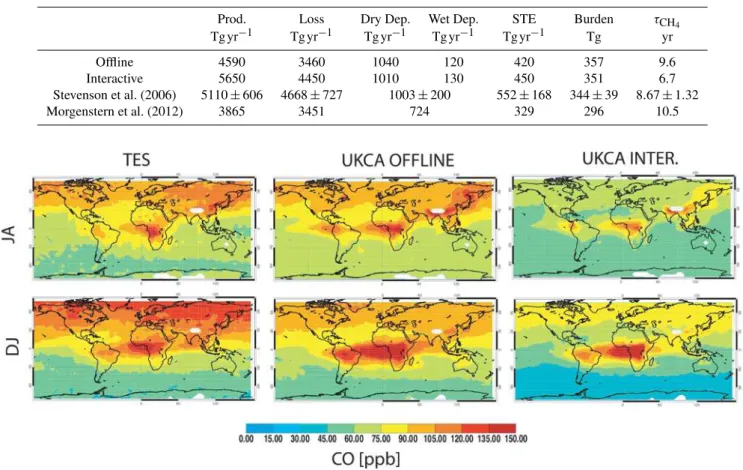
Next we compare the carbon monoxide distributions be-tween the model, with interactive and offline photolysis schemes, and the TES observations (Luo et al., 2007; Lopez et al., 2008) (Fig. 5). Again we compare for the periods July to August and January to February.
The differences between the two versions of the model are now more dramatic. Again both versions capture the broad features with high values of carbon monoxide pro-duced by biomass burning, in particular from Africa, and an-thropogenic emissions from Asia. However whilst the model with offline photolysis has only a small bias (2 %), when the interactive photolysis is employed there is a large neg-ative bias (−24 %). Although there are small positive biases
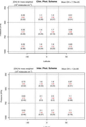
(less than 10 %) in the tropics and small negative biases in midlatitudes (less than 10 %) in the observations (Luo et al., 2007; Lopez et al., 2008), this model bias is significant. As the emissions are unchanged between the two models, we ascribe these changes to the main sink of CO and its reac-tion with the hydroxyl radical, OH. Indeed if we look at the methane lifetime (Table 3), which is dominated by its reac-tion with OH, we see that this is greatly reduced by switch-ing from the offline to interactive photolysis scheme. We can look directly at the changes in the OH by plotting the OH field, weighted as in Lawrence et al. (2001), with the offline and interactive photolysis schemes (Fig. 6).
We first note that the use of the interactive photolysis scheme increases the total OH burden, which explains the de-creased CO concentrations and CH4lifetimes. We also note
Table 3.Ozone Budget in the troposphere as defined by the tropopause of Hoerling et al. (1993) .
Prod. Loss Dry Dep. Wet Dep. STE Burden τCH4
Tg yr−1 Tg yr−1 Tg yr−1 Tg yr−1 Tg yr−1 Tg yr
Offline 4590 3460 1040 120 420 357 9.6
Interactive 5650 4450 1010 130 450 351 6.7
Stevenson et al. (2006) 5110±606 4668±727 1003±200 552±168 344±39 8.67±1.32
Morgenstern et al. (2012) 3865 3451 724 329 296 10.5
Fig. 5.Carbon Monoxide (ppbv) averaged over 800–400 hPa from 2005–2008 July/August (top row) and December/January (bottom row).
Left column: observations from TES. Middle column: model with offline photolysis. Right column: model with interactive photolysis.
that the amount of OH is excessive. To understand the in-crease we examined the production and loss terms of HOx
(≡OH+HO2) and found that the increases in HOxare
dom-inated by increases in its production via O(1D)+H2O. The
water vapour is constant between the two simulations and in a recent study found to compare reasonably well with other models and observations (Russo et al., 2011). There-fore the increase must arise from increased production of O(1D), which is produced from the photolysis of ozone. This is greatly increased by using the interactive scheme as can be seen from Fig. 3. However we believe that the increased
j (O(1D))is realistic.
The apparently superior performance of the offline pho-tolysis scheme is a result of two conflicting factors, the high bias in ozone and the low bias in the ozone photoly-sis rates. Removing one of these factors, although an im-provement in itself, thus worsens the performance of some aspects of the model. Indeed Morgenstern et al. (2012) see no such problems with high biases in OH despite using this implementation of the interactive photolysis scheme, albeit with a considerably different chemistry scheme. Results from a more complete whole atmospheric chemistry (Archibald
et al., 2012) also indicate lower ozone concentrations pro-duce lower OH concentrations, higher CO concentrations and a longer methane lifetime.
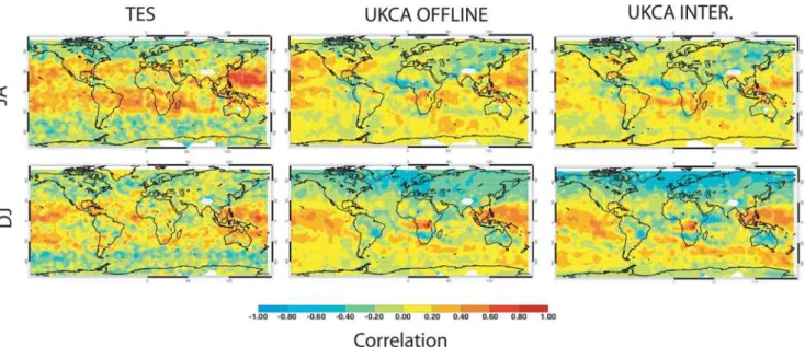
Finally, adopting the approach of Voulgarakis et al. (2011), we compare the O3–CO correlations using them to
under-stand the models’ performance (Fig. 7). Like previous ver-sions of the model (Voulgarakis et al., 2011) the O3–CO
Table 4.Photolysis reactions employed in MetUM Fast-JX and the source of their corresponding absorption cross sections.
Reaction Notes Reference
1. O2→O(3P)+O(1D) Cross section 0 in Fast-JX wavelengths.
2. O2→O(3P)+O(3P) T-dependence between 180 and 300 K. Prather et al. (2010).
3. O3→O2+O(1D) T-dependence between 180 and 300 K. Prather et al. (2010).
4. O3→O2+O(3P) T-dependence between 180 and 300 K. Prather et al. (2010).
5. NO→N+O(3P) Prather et al. (2010).
6. NO2→NO+O(3P) T-dependence between 220 and 298 K. Prather et al. (2010).
7. NO3→NO+O2 T-dependence between 190 and 300 K. Sander et al. (2006).
8. NO3→NO2+O(3P) T-dependence between 190 and 300 K. Sander et al. (2006).
9. N2O5→NO3+NO2 T-dependence between 230 and 300 K. Sander et al. (2006).
10. HONO→OH+NO Sander et al. (2006).
11. HONO2→OH+NO2 T-dependence between 200 and 300 K. Sander et al. (2006).
12. HO2NO2→HO2+NO2 T-dependence between 200 and 300 K. Sander et al. (2006).
Includes IR photolysis of Jim´enez et al. (2005).
13. N2O→N2+O(1D) T-dependence between 200 and 300 K. Prather et al. (2010).
14. H2O→OH+H Sander et al. (2006).
15. CH4→CH3OO+H Cross section 0 in Fast-JX wavelengths.
16. CO2→CO+O(3P) T-dependence between 195 and 295 K. Parkinson et al. (2003).
17. H2O2→OH+OH T-dependence between 200 and 300 K. Prather et al. (2010).
18. HCHO→HO2+HO2+CO T-dependence between 223 and 293 K. Prather et al. (2010).
19. HCHO→H2+CO T-dependence between 223 and 293 K. Prather et al. (2010).
20. CH3OOH→HO2+HCHO+OH Sander et al. (2006).
21. CH3CHO→CH3OO+HO2+CO Sander et al. (2006).
22. CH3CHO→CH4+CO Sander et al. (2006).
23. C2H5CHO→C2H35OO+HO2+CO Sander et al. (2006).
24. C2H5CHO→CH3OH+HO2+OH Sander et al. (2006).
25. CH3O3H→CH3OO+OH Sander et al. (2006).
26. (CH3)2CO→CH3CO3+CH3OO Using scheme of Blitz et al. (2004). Prather et al. (2010).
27. n−PrOOH→C2H5CHO+HO2+OH Use cross sections from reaction 20.
28. i−PrOOH→(CH3)2CO+HO2+OH Use cross sections from reaction 20.
29. CH3COCH2OOH→CH3CO3+HCHO+OH Use cross sections from reaction 20.
30. HACET→CH3CO3+HCHO+HO2 Lumped species of C3 carbonyls, including hyd- Sander et al. (2006).
roxyacetone. Use hydroxyacetone cross sections.
31. MGLY→CH3CO3+CO+HO2 Lumped species of C3 aldehydes, including IUPAC datasheet P6a
methyl glyoxal. Use methylglyoxal cross sections.
32. MACR→CH3CO3+HCHO+CO+HO2 Lumped species of C4 carbonyls, including meth- Prather et al. (2010).
acrolein. Use methacrolein cross sections. 33. MACROOH→0.5HACET+0.5CO Use cross sections from reaction 20.
+0.5MGLY+0.5HCHO+OH+HO2
34. iSOOH→MACR+HO2+HCHO+OH Use cross sections from reaction 20.
35. CH3ONO2→HO2+HCHO+NO2 T-dependence between 240 and 300 K. Prather et al. (2010).
36. PAN→CH3CO3+NO2 T-dependence between 250 and 300 K. Prather et al. (2010).
37. PPAN→C2H5CO3+NO2 Use cross sections from reaction 36.
38. MPAN→MACRO2+NO2 Use cross sections from reaction 36.
39. NALD→HCHO+CO+NO2+CO2 Use cross sections from reaction 21.
40. ISON→NO2+MACR+HCHO+NO2 Lumped species. Usei−C3H7ONO2 IUPAC datasheet P17b T-dependence between 230 and 360 K.
41. CH3Br→Br+H T-dependence between 196 and 296 K. Prather et al. (2010).
42. BrCl→Br+Cl T-dependence between 190 and 300 K. Sander et al. (2006).
43. BrO→Br+O(3P) Sander et al. (2006).
44. HOBr→Br+OH Prather et al. (2010).
45. BrNO3→Br+NO3 Sander et al. (2006).
46. BrNO3→BrO+NO2 Sander et al. (2006).
47. CFCl3→Cl+Cl+Cl Prather et al. (2010).
48. CF2Cl2→Cl+Cl Prather et al. (2010).
49. HCl→H+Cl Sander et al. (2006).
50. HOCl→Cl+OH Prather et al. (2010).
51. OClO→ClO+O(3P) Sander et al. (2006).
52. Cl2O2→Cl+Cl+O2 Sander et al. (2006).
53. ClNO3→Cl+NO3 Prather et al. (2010).
54. ClNO3→ClO+NO2 Prather et al. (2010).
ahttp://www.iupac-kinetic.ch.cam.ac.uk/datasheets/pdf/P6 CH3COCHO+hv.pdf
ï50 0 50
Clim. Phot. Scheme
Latitude
Pressure (hP
a)
[OH] Air mass weighted
(106 molecules cm<3)
Mean OH = 7.79e+05
1000
750
500
250
0.33 1.6 1.9 0.63
0.33 1.4 1.7 0.56
0.35 1.1 1.3 0.51
0.47 1.44 1.52 0.76
0.72 2 1.99 0.88
0.64 1.43 1.36 0.64
(0.36) (0.24) (0.23) (0.52)
(0.29) (0.24) (0.19) (0.39)
(0.22) (0.26) (0.27) (0.31)
ï50 0 50
Inter. Phot. Scheme
Latitude
Pressure (hP
a)
[OH] Air mass weighted (106 molecules cm<3)
Mean OH = 1.2e+06
1000
750
500
250
0.53 2.1 2.7 1.1
0.64 2.1 2.5 1.1
0.72 1.6 1.9 0.97
0.47 1.44 1.52 0.76 0.72 2 1.99 0.88 0.64 1.43 1.36 0.64
(0.46) (0.27) (0.23) (0.79)
(0.45) (0.3) (0.2) (0.58)
(0.32) (0.23) (0.24) (0.41)
Fig. 6.OH distribution, weighted as in (Lawrence et al., 2001), as
a function of height and latitude. The black numbers are the model values, the red numbers are from the Spivakovsky et al. (2000) cli-matology (obtained from Lamarque et al., 2012) and the numbers in brackets the standard deviation of the grid cell values used to ob-tain the average in the model. Top plot with offline photolysis and bottom plot with interactive photolysis.
5.2.5 Conclusions with regards to tropospheric run
We have evaluated the performance of the Fast-JX photoly-sis scheme in the tropospheric version of the MetUM model using a nudged run between 2004 and 2008. After briefly checking that nudging of the ERA-Interim analyses is suc-cessful, and that the modelled cloud optical depths were re-alistic, we proceeded to demonstrate improvements to the modelled photolysis rates using data comparisons from the INTEX-NA campaign. These results showed that the on-line photolysis model provides a significantly better descrip-tion of the observed rates. We then investigated the effects that these improved photolysis rates have on the modelled chemical fields, comparing the changes to observations from the TES satellite instrument. The improved photolysis rates, whilst producing some improvements to the chemical fields,
produced a high bias in the global burden of OH, which itself affected CO concentrations and the CH4 lifetime. This was
a result of the more realistic photolysis rates increasing the sensitivity of the model to high biases in ozone, the effects of which were masked in the offline photolysis scheme by too small ozone photolysis rates.
5.3 Stratospheric chemistry
In addition to testing the model in the troposphere, a further simple validation was performed in the stratosphere. In order to test the feedback from chemical changes onto the dynam-ics we ran the model unconstrained by nudging. The run we perform is similar to that used in Morgenstern et al. (2009), which itself follows the definition of the REF-B0 experiment of the CCMVal model intercomparison (Eyring et al., 2010). This uses forcings that represent perpetual 2000 conditions, although, as we are able to initialise the chemical fields from those in Morgenstern et al. (2009) we only perform a 10 yr run, discarding the first five years as “spin-up”.
In Fig. 8 we examine the average annual cycle of the to-tal ozone column. The values from the model are compared to a combination of data from a variety of sources including TOMS, SBUV, GOME and OMI, for the year 2000 (Bodeker et al., 2005). The model captures most of the features includ-ing the latitudinal gradient and timinclud-ing and magnitude of the Northern Hemisphere spring maximum.
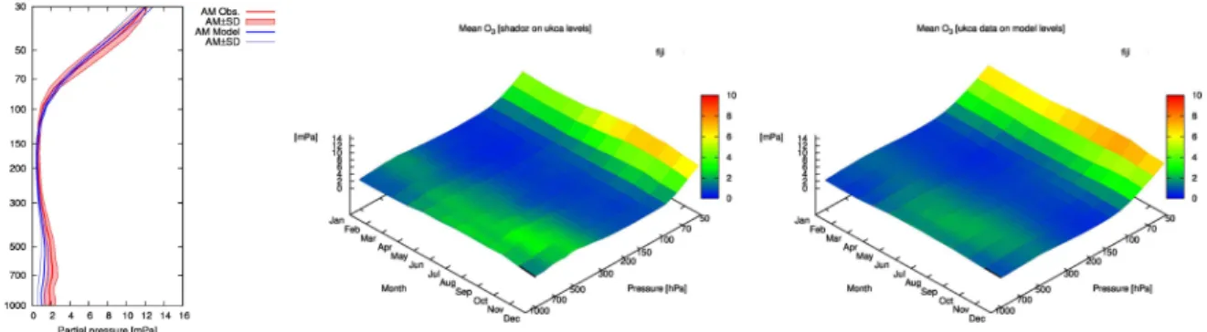
The previous version of the chemistry scheme had some discrepancies with observations around the tropopause, in-cluding high biases in temperature and ozone (Morgenstern et al., 2009). To assess how the updated model performs we compare ozone profiles with those from the SHADOZ net-work (Thompson et al., 2003a,b). We show results from one representative site, Fiji, in Fig. 9 displaying monthly mean ozone profiles as a function of pressure. The model is able to capture the seasonal cycle well, though it does still slightly overestimate UTLS ozone. Tropospheric ozone is slightly low, as should be expected, as this version of the model does not attempt to fully simulate tropospheric emissions and chemistry.
6 Discussion
Fig. 7.Correlation between “free tropospheric” (800–400 hPa) Ozone and Carbon Monoxide from 2005–2008 July/August (top row) and December/January (bottom row). Left column: observations from TES. Middle column: model with offline photolysis. Right column: model with interactive photolysis.
Fig. 8.Comparison between assimilated total ozone column data
(Bodeker et al., 2005) (lines) and the stratospheric chemistry model (filled coloured contours).
can be seen with both photolysis schemes when compared to the TES satellite instrument data in Fig. 4.
We have reduced the O3high bias by various measures,
including the replacement of the original upper boundary condition for NOyas used by O’Connor et al. (2009) with
one from the Cambridge-2D model, adding the additional re-action between HO2 and NO using the rates and yields of
Butkovskaya et al. (2007) and adding the hydrolysis of N2O5
(Morgenstern et al., 2009). Whilst these reduced the biases in ozone they did not eliminate them. Further work is being carried out at present to try and understand the sources of these biases, but they cannot obscure the improved
descrip-tion of observed photolysis rates by the interactive photolysis scheme as opposed to the offline scheme.
Even with the removal of the high biases in ozone there are still ways of expanding the capability of the interactive pho-tolysis scheme. One obvious omission is the limited use of aerosols in the model. This will change when the GLOMAP-mode scheme (Mann et al., 2010) is coupled to the photol-ysis. Although on a global scale aerosols are less important than clouds for the optical depth calculation, there are lo-calised regions where this coupling will be useful. A further improvement, of greater importance for the stratosphere, will be the use of a variable solar constant, a driver of some of the variability in stratospheric ozone. Whilst our simple ap-proach of accounting for overlapping cloud layers seems to work at present, increasing vertical resolution may require more sophisticated techniques to be employed (Neu et al., 2007). The new methods of sampling the model, expanding the data sets it can be validated against, will also be useful in assessing other aspects of the model performance.
7 Conclusions
Fig. 9.Comparison of monthly mean O3profiles between the stratospheric version of the chemistry model and sondes from the SHADOZ network over an example site, in this case Fiji (18◦S, 178◦E). The left-hand plot shows annual mean profiles in the model and in the observations. The right-hand plots resolve the variation over the year in observations (left) and the model (right).
the interactive photolysis scheme. As well as being a more realistic manner of modelling, the photolysis the interactive scheme will permit more detailed studies of the interactions between the atmosphere and its constituents.
Acknowledgements. We acknowledge NCAS and NCEO for their
funding of this work. MD and FMOC were supported by the Joint DECC/Defra Met Office Hadley Centre Climate Programme (GA01101).
We thank Michael Prather for the provision of the Fast-JX code and Oliver Wild and Apostolos Voulgarakis for insights into its op-eration. We thank Martyn Chipperfield for his help in comparing the PHOTOCOMP model intercomparison. We thank Glenn Carver and Nick Savage for discussions about the flight track sampling code. We thank Maria Russo for discussions about water vapour and clouds. We acknowledge James Keeble for his work in assist-ing understandassist-ing of the updated stratospheric chemistry.
Biogenic emissions were obtained from the GEIA
cen-tre http://www.geiacenter.org/inventories/present.html. The
INTEX-A data was obtained from the NASA-LARC website http://www-air.larc.nasa.giv/missions/intexna/intexna.htm. The IS-CCP D2 data/images were obtained from the International Satellite Cloud Climatology Project web site http://isccp.giss.nasa.gov main-tained by the ISCCP research group at the NASA Goddard Institute for Space Studies, New York, NY on March, 2010 (Rossow and Schiffer, 1999). We would like to thank Greg Bodeker of Bodeker Scientific for providing the combined total column ozone database (http://www.bodekerscientific.com/data/total-column-ozone). We thank the NASA Langley Research Center Atmospheric Science Data Center for the TES data.
Edited by: A. Stenke
References
Aghedo, A. M., Bowman, K. W., Shindell, D. T., and Falu-vegi, G.: The impact of orbital sampling, monthly averaging and vertical resolution on climate chemistry model evaluation
with satellite observations, Atmos. Chem. Phys., 11, 6493–6514, doi:10.5194/acp-11-6493-2011, 2011.
Archibald, A. T., Abraham, N. L., Braesicke, P., Dalvi, M., Johnson, C., Keeble, J. M., O’Connor, F. M., Squire, O. J., Telford, P. J., and Pyle, J. A.: Evaluation of the UM-UKCA model configura-tion for Chemistry of the Stratosphere and Troposphere (CheST), Geosci. Model Dev., in preparation, 2012.
Beer, R., Glavic, T., and Rider, M.: Tropospheric emission spec-trometer for the Earth observing System’s Aura Satellite, Appl. Optics, 40, 2356–2367, 2001.
Bellouin, N., Boucher, O., Haywood, J., Johnson, C., Jones, A., Rae, J., and Woodward, S.: Improved representation of aerosols for HadGEM2, Tech. rep., Met Office Hadley Centre, 2007. Bian, H. and Prather, M.: Fast-J2: accurate simulation of
strato-pheric photolysis in global chemical models, J. Atmos. Chem., 41, 281–296, 2002.
Blitz, M., Heard, D., and Pilling, M.: Pressure and temperature-dependent quantum yields for the photodissociation of acetone between 279 and 327.5 nm, Geophys. Res. Lett., 31, L06111, doi:10.1029/2003GL018793, 2004.
Bodeker, G. E., Shiona, H., and Eskes, H.: Indicators of Antarc-tic ozone depletion, Atmos. Chem. Phys., 5, 2603–2615, doi:10.5194/acp-5-2603-2005, 2005.
Briegleb, P.: Delta-eddington approximation for solar radiation in the ncar community climate models, J. Geophys. Res., 97, 7603– 7612, 1992.
Butkovskaya, N. I., Kukui, A., and Le Bras, G.: HNO3 forming channel of the HO2+N Oreaction as a function of pressure and temperature in the ranges of 72–600 Torr and 223–323 K, J. Phys. Chem. A, 111, 9047–9053, 2007.
Chipperfield, M., Kinnison, D., Bekki, S., Bian, H., Br¨uhl, C., Canty, T., Cionni, I., Dhomse, S., Froidevaux, L., Fuller, R., M¨uller, R., Prather, M., Salawitch, R., Santee, M., Tian, W., and Tilmes, S.: SPARC CCMVal Report on the Evaluation of Chemistry-Climate Models, Stratospheric Chemistry, chapter 6, 191–252, SPARC, http://homepages.see.leeds.ac.uk/∼lecmc/
ccmvalj/, 2010.
Dee, D., Uppala, S., Simmons, A., Berrisford, P., Poli, P., Kobayashi, S., Andrae, U., Balmaseda, M. A., Balsamo, G., Bauer, P., Bechtold, P., Beljaars, A. C. M., van de Berg, L., Bid-lot, J., Bormann, N., Delsol, C., Dragani, R., Fuentes, M., Geer, A. J., Haimberger, L., Healy, S. B., Hersbach, H., H´olm, E. V., Isaksen, L., K˚allberg, P., K¨ohler, M., Matricardi, M., McNally, A. P., Monge-Sanz, B. M., Morcrette, J.-J., Park, B.-K., Peubey, C., de Rosnay, P., Tavolato, C., Th´epaut, J.-N., and Vitart, F.: The ERA-Interim reanaysis: configurationa and performance of the data analysis system, Q. J. Roy. Meteor. Soc., 137, 553–597, doi:10.1002/qj.828, 2011.
Edwards, J. and Slingo, A.: Studies with a flexible new radiation code. I: Choosing a configuration for a large-scale model, Q. J. Roy. Meteor. Soc., 122, 689–719, 1996.
Edwards, J. M., Havemann, S., Thelen, J.-C., and Baran, A.: A new parameterisation for the radiative properties of ice crystals, com-parison of existing schemes and impact in a GCM, Atmos. Res., 83, 19–35, doi:10.1016/j.atmosres.2006.03.002, 2007.
Eyers, C., Addleton, D., Atkinson, K., Broomhead, M., Chris-tou, R., Elliff, T., Falk, R., Gee, I., Lee, D., Marizy, C., Michot, S., Middel, J., Newton, P., Norman, P., Plohr, M., Raper, D., and Stanciou, N.: AERO2K global aviation emissions inventories for 2002 and 2025, Tech. Rep. 04/01113, Qinetiq, http://aero-net.info/fileadmin/aeronet files/links/documents/ AERO2K Global Aviation Emissions Inventories for 2002 and 2025.pdf, 2004.
Eyring, V., Shepherd, T., and Waugh, D.: SPARC Report on the Evaluation of Chemistry-Climate Models, Tech. rep., SPARC Report No. 5, WCRP-132, WMO/TD-N0. 1526, http://www. atmosp.physics.utoronto.ca/SPARC/ccmval final/index.php, 2010.
Feng, Y., Penner, J. E., Sillman, S., and Liu, X.: Effects of cloud overlap in photochemical models, J. Geophys. Res., 109, D04310, doi:10.1029/2003JD004040, 2004.
Fitzgerald, J.: Approximation formulas for the equilibrium size of an aerosol particle as a function of its dry size and composition and the ambient relative humid-ity, J. Appl. Meteorol., 14, 1044–1049, doi:10.1175/1520-0450(1975)014<1044:AFFTES>2.0.CO;2, 1975.
Giannakopoulos, C., Chipperfield, M., Law, K., and Pyle, J.: Valida-tion and intercomparison of wet and dry deposiValida-tion schemes us-ing Pb-210 in a global three-dimensional off-line chemical trans-port model, J. Geophys. Res., 104, 23761–23784, 1999. Guenther, A., Hewitt, C. N., Erickson, D., Fall, R., Geron, C.,
Graedel, T., Harley, P., Klinger, L., Lerdau, M., McKay, W. A., Pierce, T., Scoles, B., Steinbrecher, R., Tallaamraju, R., Tay-lor, J., and Zimmerman, P.: A global model of natural volatile organic compound emissions, J. Geophys. Res., 100, 8873–8892, 1995.
Hewitt, H. T., Copsey, D., Culverwell, I. D., Harris, C. M., Hill, R. S. R., Keen, A. B., McLaren, A. J., and Hunke, E. C.: De-sign and implementation of the infrastructure of HadGEM3: the next-generation Met Office climate modelling system, Geosci. Model Dev., 4, 223–253, doi:10.5194/gmd-4-223-2011, 2011. Hoerling, M., Schaack, T., and Lenzen, A.: A global analysis
of stratospheric-tropospheric exchange during northern winter, Mon. Weather Rev., 121, 162–172, 1993.
Hough, A. M.: The calculation of photolysis rates for use in global modelling studies, Tech. rep., UK Atomic Energy Authority,
Har-well, Oxon., UK, 1988.
Jim´enez, E., Gierczak, T., Stark, H., Burkholder, J. B., and Ravis-hankara, A. R.: Quantum yields of OH, HO2and NO3in the UV photolysis of HO2NO2, Phys. Chem. Chem. Phys., 7, 342–348, 2005.
Kenner, R. D., Rohrer. F., and Stuhl, F.: Hydroxyl (A) production in the 193-nm photolysis of nitrous acid, J. Phys. Chem., 90, 2635– 2639, 1986.
Kipling, Z., Stier, P., Schwarz, J. P., Perring, A. E., Spackman, J. R., Mann, G. W., Johnson, C. E., and Telford, P. J.: Constraints on aerosol processes in climate models from vertically-resolved aircraft observations of black carbon, Atmos. Chem. Phys. Dis-cuss., 13, 437–473, doi:10.5194/acpd-13-437-2013, 2013. Lamarque, J.-F., Bond, T. C., Eyring, V., Granier, C., Heil, A.,
Klimont, Z., Lee, D., Liousse, C., Mieville, A., Owen, B., Schultz, M. G., Shindell, D., Smith, S. J., Stehfest, E., Van Aar-denne, J., Cooper, O. R., Kainuma, M., Mahowald, N., Mc-Connell, J. R., Naik, V., Riahi, K., and van Vuuren, D. P.: His-torical (1850–2000) gridded anthropogenic and biomass burning emissions of reactive gases and aerosols: methodology and ap-plication, Atmos. Chem. Phys., 10, 7017–7039, doi:10.5194/acp-10-7017-2010, 2010.
Lamarque, J.-F., Emmons, L. K., Hess, P. G., Kinnison, D. E., Tilmes, S., Vitt, F., Heald, C. L., Holland, E. A., Lauritzen, P. H., Neu, J., Orlando, J. J., Rasch, P. J., and Tyndall, G. K.: CAM-chem: description and evaluation of interactive atmospheric chemistry in the Community Earth System Model, Geosci. Model Dev., 5, 369–411, doi:10.5194/gmd-5-369-2012, 2012. Lary, D. and Pyle, J.: Diffuse-radiation, twilight, and
photochem-istry, J. Atmos. Chem., 13, 393–406, 1991.
Law, K. and Pyle, J.: Modeling trace gas budgets in the troposphere 1. ozone and odd nitrogen, J. Geophys. Res., 98, 18377–18400, 1993a.
Law, K. and Pyle, J.: Modeling trace gas budgets in the troposphere 2. CH4and CO, J. Geophys. Res., 98, 18401–18412, 1993b. Law, K., Plantevin, P., Shallcross, D., Rogers, H., Pyle, J.,
Grouhel, C., Thouret, V., and Marenco, A.: Evaluation of
mod-eled O3 using Measurement of Ozone by Airbus In-Service
Aircraft (MOZAIC) data, J. Geophys. Res., 103, 25721–25737, 1998.
Lawrence, M. G., J¨ockel, P., and von Kuhlmann, R.: What does the global mean OH concentration tell us?, Atmos. Chem. Phys., 1, 37–49, doi:10.5194/acp-1-37-2001, 2001.
Liu, H., Crawford, J., Pierce, R., Norris, P., Platnick, S., Chen, G., Logan, J., Yantosca, R., Evans, M., Kittaka, C., Feng, Y., and Tie, X.: Radiative eddect of clouds on tropspheric chemistry in a global three-dimensional chemical transport model, J. Geo-phys. Res., 111, D20303, doi:10.1029/2005JD006403, 2006. Lopez, J. P., Luo, M., Christensen, L. E., Loewenstein, M., Jost, H.,
Webster, C. R., and Osterman, G.: TES carbon monoxide valida-tion during two AVE campaigns using the Argus and ALIAS in-struments on NASA’s WB-57F, J. Geophys. Res., 113, D16847, doi:10.1029/2007JD008811, 2008.
Mann, G. W., Carslaw, K. S., Spracklen, D. V., Ridley, D. A., Manktelow, P. T., Chipperfield, M. P., Pickering, S. J., and Johnson, C. E.: Description and evaluation of GLOMAP-mode: a modal global aerosol microphysics model for the UKCA composition-climate model, Geosci. Model Dev., 3, 519–551, doi:10.5194/gmd-3-519-2010, 2010.
Marchand, R., Ackerman, T., Smyth, M., and Rossow, W. B.: A re-view of cloud top height and optical depth histograms from MISR, ISCCP, and MODIS, J. Geophys. Res., 115, D16206, doi:10.1029/2009JD013422, 2010.
Morgenstern, O., Braesicke, P., O’Connor, F. M., Bushell, A. C., Johnson, C. E., Osprey, S. M., and Pyle, J. A.: Evaluation of the new UKCA climate-composition model – Part 1: The strato-sphere, Geosci. Model Dev., 2, 43–57, doi:10.5194/gmd-2-43-2009, 2009.
Morgenstern, O., Zeng, G., Abraham, N., Telford, P., Braesicke, P., Pyle, J., Hardiman, S. C., O’Connor, F. M., and Johnson, C. E.: Impacts of climate change, ozone recovery, and increasing methane on the tropospheric oxodising capacity, J. Geophys. Res., doi:10.1029/2012JD018382, in press, 2012.
Nassar, R., Logan, J. A., Worden, H. M., Megretskaia, I. A., Bow-man, K. W., OsterBow-man, G. B., Thompson, A. M., Tarasick, D. W., Austin, S., Claude, H., Manvendra, K., Dubey, W., Hock-ing, K., Johnson, B. J., Joseph, E., Merrill, J., Morris, G. A., Newchurch, M., Oltmans, S. J., Posny, F., Schmidlin, F. J., V¨omel, H., Whiteman, D. N., and Witte, J. C.: Validation of Tro-pospheric Emission Spectrometer (TES) nadir ozone profiles us-ing ozonesonde measurements, J. Geophys. Res., 113, D15S17, 13 pp., doi:10.1029/2007JD008819, 2008.
Neu, J., Prather, M., and Penner, J.: Global atmospheric chemistry: integrating over fractional cloud cover, J. Geophys. Res., 112, D11306, 12 pp., doi:10.1029/2006JD008007, 2007.
O’Connor, F., Carver, G., Savage, N., Pyle, J. A., Methven, J., Arnold, S. R., Dewey, K., and Kent, J.: Comparison and visual-isation of high resolution transport modelling with aircraft mea-surements, Atmos. Sci. Lett., 6, 164–170, doi:10.1002/asl.111, 2005.
O’Connor, F., Johnson, C., Morgenstern, O., and Collins, W. J.: Interactions between tropospheric chemistry and climate model temperature and humidity biases, Geophys. Res. Lett, 36, L16801, doi:10.1029/2009GL039152, 2009.
O’Connor, F. M., Johnson, C. E., Morgenstern, O., Abraham, N. L., Braesicke, P., Dalvi, M., Folberth, G. A., Sanderson, M. G., Telford, P. J., Young, P. J., Zeng, G., Collins, W. J., and Pyle, J. A.: Evaluation of the new UKCA climate-composition model, Part II. The Troposphere, Geosci. Model Dev. Discuss., in review, 2013.
Parkinson, W., Rufus, J., and Yoshino, K.: Absolute absorption cross section measurements of CO2 in the wavelength region 163–200 nm and the temperature dependence, Chem. Phys., 290, 251–256, 2003.
P¨oschl, U., von Kuhlmann, R., Poisson, N., and Crutzen, P.: De-velopment and intercomparison of condensed isoprene oxidation mechanisms for global atmospheric modelling, J. Atmos. Chem., 37, 29–52, 2000.
Price, C. and Rind, D.: Modelling global lightning distributions in a general circulation model, Mon. Weather Rev., 122, 1930– 1939, 1994.
Rayner, A., Rayner, N., Parker, D., Horton, E., Folland, C., Alexan-der, L., Rowell, D., Kent, E., and Kaplan, A.: Global analyses of sea surface temperature, sea ice, and night marine air tem-perature since the late nineteenth century, J. Geophys. Res., 108, 4407, 29 pp., doi:10.1029/2002JD002670, 2003.
Richards, N. A. D., Osterman, G. B., Browell, E. V., Hair, J. W., Av-ery, M., and Li, Q.: Validation of Tropospheric Emission Spec-trometer ozone profiles with aircraft observations during the intercontinental chemical transport experiment-B, J. Geophys. Res.-Atmos., 113, D16S29, doi:10.1029/2007jd008815, 2008. Rodgers, C. D. and Connor, B. J.: Intercomparison of remote
sounding instruments, J. Geophys. Res.-Atmos., 108, 4116, doi:10.1029/2002jd002299, 2003.
Rossow, W., Walker, A., Beuschel, D., and Roiter, M.: International Satellite Cloud Climatology Project (ISCCP) Documentation of New Cloud Datasets, Tech. rep., World Meteorological Or-ganization, http://isccp.giss.nasa.gov/pub/documents/d-doc.pdf, 1996.
Rossow, W. B. and Schiffer, R. A.: Advances in understanding clouds from ISCCP, B. Am. Meteorol. Soc., 80, 2261–2287, 1999.
Russo, M. R., Mar´ecal, V., Hoyle, C. R., Arteta, J., Chemel, C., Chipperfield, M. P., Dessens, O., Feng, W., Hosking, J. S., Telford, P. J., Wild, O., Yang, X., and Pyle, J. A.: Representa-tion of tropical deep convecRepresenta-tion in atmospheric models – Part 1: Meteorology and comparison with satellite observations, At-mos. Chem. Phys., 11, 2765–2786, doi:10.5194/acp-11-2765-2011, 2011.
Sander, S., Friedl, R., Golden, D., Kurylo, M. J., Huie, R., Orkin, V., Moortgat, G., Ravishankra, A., Kolb, C., Molina, M., and Finlayson-Pitts, B.: Chemical Kinetics and Photochemical Data for Use in Atmospheric Studies Evaluation Number 14, Tech. rep., JPL, http://jpldataeval.jpl.nasa.gov/pdf/JPL 02-25 rev02.pdf, 2003.
Sander, S., Friedl, R., Golden, D. M., Kurylo, M., Moortgat, G., Keller-Rudek, H., Wine, P., Ravishankra, A. R., Kolb, C., Molina, M., Finlayson, B., Huie, R., and Orkin, V.: Chemical Ki-netics and Photochemical Data for Use in Atmospheric Studies Evaluation Number 15, Tech. rep., NASA JPL, http://jpldataeval. jpl.nasa.gov/pdf/JPL 15 AllInOne.pdf, 2006.
Shetter, R. E. and M¨uller, M.: Photolysis frequency measurements using actinic flux spectroradiometry during the PEM-Tropics mission: Instrumentation description and some result, J. Geo-phys. Res., 104, 5647–5661, 1999.
Singh, H. B., Crawford, J. H., Jacob, D. J., and Russell, P. B.: Overview of the summer 2004 Intercontinental Chemical Trans-port Experiment–North America (INTEX-A), J. Geophys. Res., 111, D24S01, doi:10.1029/2006JD007905, 2006.
Slingo, A.: A GCM parameterization for the shortwave radiative properties of water clouds, J. Atmos. Sci., 46, 1419–1427, 1989. Spivakovsky, C., Logan, J., Montzka, S., Balkanski, Y., Foreman-Fowler, M., Jones, D., Horowitz, L., Fusco, A., Brenninkmei-jer, C., Prather, M., Wofsy, S., and McElroy, M.: Three-dimensional climatological distribution of tropospheric OH: up-date and evaluation, J. Geophys. Res., 105, 8931–8980, 2000. Stevenson, D., Dentener, F., Schultz, M., Ellingsen, K., van
Hauglustaine, D., Horowitz, L., Isaksen, I., Krol, M., Lamar-que, J.-F., Lawrence, M., Montanaro, V., ller, J.-F. M., Pitari, G., Prather, M., Pyle, J., Rast, S., Rodriguez, J., Sanderson, M., Savage, N., Shindell, D., Strahan, S., Sudo, K., and Szopa, S.: Multimodel ensemble simulations of present-day and near-future tropospheric ozone, J. Geophys. Res., 111, D08301, 23 pp., doi:10.1029/2005JD006338, 2006.
Stutz, J., Kim, E. S., Platt, U., Bruno, P., Perrino, C., and Febo, A.: UV-visible absorption cross sections of nitrous acid, J. Geophys. Res., 105, 14585–14592, 2000.
Telford, P. J., Braesicke, P., Morgenstern, O., and Pyle, J. A.: Tech-nical Note: Description and assessment of a nudged version of the new dynamics Unified Model, Atmos. Chem. Phys., 8, 1701– 1712, doi:10.5194/acp-8-1701-2008, 2008.
Telford, P. J., Lathi`ere, J., Abraham, N. L., Archibald, A. T., Braesicke, P., Johnson, C. E., Morgenstern, O., O’Connor, F. M., Pike, R. C., Wild, O., Young, P. J., Beerling, D. J., Hewitt, C. N., and Pyle, J.: Effects of climate-induced changes in isoprene emissions after the eruption of Mount Pinatubo, Atmos. Chem. Phys., 10, 7117–7125, doi:10.5194/acp-10-7117-2010, 2010. Thompson, A., Witte, J., McPeters, R., Oltmans, S., Schmidlin, F.,
Logan, J., M.Fujiwara, Kirchhoff, V., Posny, F., Coetzee, G., Hoegger, B., Kawakami, S., Ogawa, T., Johnson, B., V¨omel, H., and Labow, G.: Southern Hemisphere Additional Ozoneson-des (SHADOZ) 1998–2000 tropical ozone climatology 1. Com-parison with Total Ozone Mapping Spectrometer (TOMS) and ground-based measurements, J. Geophys. Res., 108, 8238, doi:10.1029/2001JD000967, 2003a.
Thompson, A., Witte, J., Oltmans, S., Schmidlin, F., Logan, J., Fu-jiwara, M., Kirchhoff, V., Posny, F., Coetzee, G., Hoegger, B., Kawakami, S., Ogawa, T., Fortuin, J., and Kelder, H.: South-ern Hemisphere Additional Ozonesondes (SHADOZ) 1998– 2000 tropical ozone climatology 2. Tropospheric variability and the zonal wave-one, J. Geophys. Res., 108, D28241, doi:10.1029/2002JD002241, 2003b.
Tie, X. X., Madronich, S., Walters, S., Rasch, P., and Collins, W.: Effect of clouds on photolysis and oxidants in the troposphere, J. Geophys. Res., 108, D204642, doi:10.1029/2003JD003659, 2003.
Voulgarakis, A., Savage, N. H., Wild, O., Carver, G. D., Clemit-shaw, K. C., and Pyle, J. A.: Upgrading photolysis in the p-TOMCAT CTM: model evaluation and assessment of the role of clouds, Geosci. Model Dev., 2, 59–72, doi:10.5194/gmd-2-59-2009, 2009.
Voulgarakis, A., Telford, P. J., Aghedo, A. M., Braesicke, P., Falu-vegi, G., Abraham, N. L., Bowman, K. W., Pyle, J. A., and Shin-dell, D. T.: Global multi-year O3-CO correlation patterns from models and TES satellite observations, Atmos. Chem. Phys., 11, 5819–5838, doi:10.5194/acp-11-5819-2011, 2011.
Wild, O., Zhu, X., and Prather, M.: Fast-J: accurate simulation of in- and below-cloud photolysis in tropospheric chemical models, J. Atmos. Chem., 37, 245–282, doi:10.1023/A:1006415919030, 2000.
Yienger, J. and Levy II, H.: Empirical model of global soil biogenic NOxemissions, J. Geophys. Res., 100, 11477–11464, 1995. Young, P.: The influence of Biogenic Emissions on Atmospheric
Chemistry: a Model Study for Present and Future Atmospheres, PhD thesis, University of Cambridge, http://ulmss-newton.lib. cam.ac.uk/vwebv/holdingsInfo?bibId=30191, 2007.
![Fig. 4. Ozone [ppbv] averaged over 800–400 hPa from 2005–2008 July/August (top row) and Dec/Jan (bottom row)](https://thumb-eu.123doks.com/thumbv2/123dok_br/18297016.347256/9.892.75.831.87.422/fig-ozone-ppbv-averaged-july-august-dec-jan.webp)