Assessing high altitude glacier volume change and remaining thickness using cost-efficient scientific techniques: the case of Nevado Coropuna (Peru)

(1)

TCD

3, 831–856, 2009

Assessing high altitude glacier volume change and remaining thickness

P. Peduzzi et al.

Title Page

Abstract Introduction

Conclusions References

Tables Figures

◭ ◮

Back Close

Full Screen / Esc

Printer-friendly Version

Interactive Discussion The Cryosphere Discuss., 3, 831–856, 2009

www.the-cryosphere-discuss.net/3/831/2009/ © Author(s) 2009. This work is distributed under the Creative Commons Attribution 3.0 License.

The Cryosphere Discussions

The Cryosphere Discussionsis the access reviewed discussion forum ofThe Cryosphere

Assessing high altitude glacier volume

change and remaining thickness using

cost-e

_ffi

cient scientific techniques: the

case of Nevado Coropuna (Peru)

P. Peduzzi1,2, C. Herold2, and W. Silverio3

1

Institute of Geomatics and Risk Analysis (IGAR), University of Lausanne, Switzerland

2

UNEP/GRID-Europe, 11, ch. Des An ´emones, 1219 Ch ˆatelaine, Switzerland

3

University of Geneva, Climatic Change and Climate Impacts Research Group, Institute for Environmental Sciences, University of Geneva, 7 route de Drize, 1227 Carouge, Switzerland

Received: 6 July 2009 – Accepted: 30 August 2009 – Published: 6 October 2009

Correspondence to: P. Peduzzi ([email protected])

(2)

TCD

3, 831–856, 2009

P. Peduzzi et al.

Title Page

Tables Figures

◭ ◮

Back Close

Full Screen / Esc

Interactive Discussion

Abstract

Higher temperature and change in precipitation patterns have induced an acute de-crease in Andean glaciers, thus leading to an additional stress on water supply. To adapt to climate changes, local governments need information on the rate of glacier volume losses and on current ice thickness. We show how volume changes can be

5

accurately estimated in remote areas using readily available low-cost digital elevation models derived from both topographic maps and satellite images. They were used for estimating the volume changes over the Coropuna glacier (Peru) from 1955 to 2002. Ice thickness was measured in 2004 using a georadar coupled with Ground Positioning System during a field expedition. It provided profiles of ice thickness on different slopes,

10

orientations and altitudes. These were used to model the current glacier volume us-ing Geographical Information System and statistical multiple regressions techniques. Computers were modified to resists to high altitude (6500 m) temperatures and low pressure conditions. The results delineated a significant glacier volume loss and pro-vided an estimate of the remaining ice. It propro-vided the scientific evidence needed by

15

local Peruvian NGO, COPASA, and the German Cooperation Program in order to alert local governments and communities and for enforcing new climate change adaptation policies.

1 Introduction

1.1 General context

20

Changes in glaciers and ice caps are good indicators of evidence of climate change (Zemp et al., 2008). A majority of the world glaciers have undergone a reduction in their mass at an accelerating rate (Bates et al., 2008). This is of concern given that about one-sixth of the world’s population depend on glacier and snow melting for their water supply (Stern, 2007).

(3)

TCD

3, 831–856, 2009

P. Peduzzi et al.

Title Page

Tables Figures

◭ ◮

Back Close

Full Screen / Esc

Interactive Discussion In Peru, the demographic growth and rising water demand for agriculture, domestic

and economic activities generate an increased pressure on water resources. As the rainy season is concentrated during four months of the year, the role of glaciers is cru-cial for spreading out the water supply during the dry season. Melting glaciers increase flood risk during the wet season and reduce dry-season water supplies. This is of

con-5

cern in the Indian sub-continent and parts of China as well as in the Andes (Stern, 2007). In the latter region, the glacier monitoring for the period 1970–1996 revealed an acute retreat of Andean glaciers, with glacier coverage decreasing from 725 km2in 1970 to 600 km2in 1996 (Silverio and Jaquet, 2005) in Cordilera Blanca (Peru).

1.2 Assessing change of ice volume in Nevado Coropuna (6500 m, Peru)

10

The present study on Coropuna Glacier was made at the request of the Cooperation Peruano Allemana Para la Seguridad Alementicia (COPASA, Special Project of Are-quipa Regional Government in collaboration with the German cooperation program (GTZ). They needed scientific evidences of glacier retreat in order to introduce climate change adaptation policies on water supply along with local government and

commu-15

nities.

The study was carried out by a team from UNEP/GRID-Europe and the University of Geneva. It assessed glacial retreat using both satellite imagery analysis and in situ measurements of the Coropuna Glacier.

A first analysis based on archive satellite images (Silverio, 2005) revealed that the

20

Coropuna Glacier lost 54% of its surface between 1955 and 2003. It also showed that the level of precipitation varies significantly during El Ni ˜no events. To measure the change in volume of the glacier, different Digital Elevation Models (DEM) were used. A field mission was carried out to measure ice thickness using a georadar coupled with Ground Positioning System. It provided profiles of ice thickness on different slopes,

25

(4)

TCD

3, 831–856, 2009

P. Peduzzi et al.

Title Page

Tables Figures

◭ ◮

Back Close

Full Screen / Esc

Interactive Discussion organisations, simple and low-costs techniques to follow glaciers volume dynamic and

remaining ice volume are needed. The purpose of this paper is to show how with limited budget and using locally available hardware, scientific evidences of glacier volume variation and ice thickness can be obtained.

2 Data collection

5

2.1 Study area

The Coropuna Glacier is the third highest summit in Peru, culminating at 6446 m. It is located at 15 546 S, 72 660 W, about 155 km north west of the city of Arequipa in Peru. 8000 persons depend on the Coropuna Glacier for their water supply. It is estimated that 30 000 people depend indirectly on the glacier for their livelihood.

10

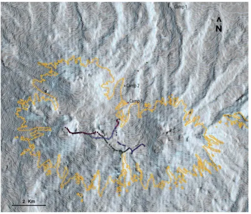
The study area covered 577 km2around the Coropuna summit. This area includes the entire glacier surface as observed in 1955. A base camp at 5664 m was set up, and ground measures were collected at altitudes ranging between 5870 and 6446 m (see Fig. 1).

2.2 Data sources

15

2.2.1 Digital elevation models

In order to estimate the ice volume loss between 1955 and today, height Digital Eleva-tion Models (DEM) from different years and periods were considered. The first one was generated (by Walter Silverio) with manually digitalised isolines from the topographic map of 1955. The one from 1997 was acquired by GTZ/COPASA from SARMAP, based

20

(5)

TCD

3, 831–856, 2009

P. Peduzzi et al.

Title Page

Tables Figures

◭ ◮

Back Close

Full Screen / Esc

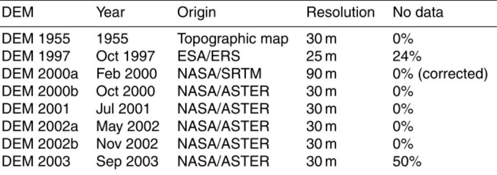
Interactive Discussion The period of data acquisition was the first criterion considered for selection. The

DEM acquired between the months of December to May were treated as lower quality, since they are likely to be influenced by the amount of snow following the rainy season. Studies were made on all DEMs but the results are based on the following three DEMs: 1955, 1997 and 2002b.

5

This choice was made based on the quality of the dataset, but also to ensure an adequate time span between the datasets. It should be noted that the DEM 2003 would have o_ffered a better time span, but since only half of the glacier was covered, it was finally rejected.

2.3 Measures from the field

10

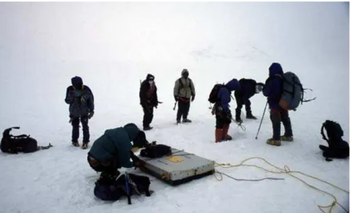
The purpose of the expedition was to measure the depth of the ice as well as tak-ing GPS points for the calibration of the DEM. The 14 day-mission was undertaken between 13 and 26 August 2004. The team was composed of two scientists and 11 support staff(guides, porters. . . ).

2.3.1 The scientific instruments

15

The scientific instruments used were selected based on local availability. The Ground Penetrating Radar (GPR) Ramac X3M, included a 100 MHz shielded antenna, batter-ies and electronic device. Much lighter GPR exists; however, we used the only GPR available in Arequipa. To avoid carrying the 35 kg antenna every day, it was protected by a waterproof bag and buried under the snow. Three Global Positioning System

re-20

(6)

TCD

3, 831–856, 2009

P. Peduzzi et al.

Title Page

Tables Figures

◭ ◮

Back Close

Full Screen / Esc

3 Methodology

3.1 Estimation of ice thickness

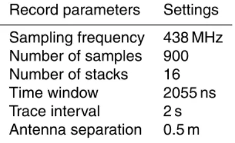
Measuring the ice volume was achieved with a GPR. The device was set to emit at 438 MHz. The signal travels through ice at 0.16 m/ns. This setting was used according to other studies performed in similar conditions (Gruber, Ludwig and Moore, 1996).

5

The depth of ice can be measured by recording the time lag between the emission and the reception of the signal (see Eq. 1)

I=T/(2C) (1)

where

I=Ice thickness [m]

10

T =Time [ns]

C=Speed of propagation through ice of the signal (0.16 [m/ns])

For example a time lag of 2000 ns=160 m of ice thickness. Technical settings are specified in Table 2. This allows the detection of the bedrock. Figure 2 illustrates the

15

set up used during the collection of the data.

Each recorded depth was coupled with geographical coordinates obtained using a GPS so that the profiles could be geo-referenced. Given time and access constraints, it was not possible to achieve a comprehensive recording of the glacier surface. Hence, the mission included several transects lines. The selected targets were chosen to

20

(7)

TCD

3, 831–856, 2009

P. Peduzzi et al.

Title Page

Tables Figures

◭ ◮

Back Close

Full Screen / Esc

3.2 Estimation of ice volume loss

Although passive satellite sensors, such as Landsat TM, provide estimate of the area covered by ice (Silverio and Jaquet, 2005). They do not provide information on the loss of ice thickness. The idea is to evaluate the thickness of ice using DEM time series.

3.2.1 Calibration and corrections

5

In order to compare different DEMs, several operations were needed. Firstly, all the DEM were re-sampled to 30 m to compensate for different spatial resolutions. They were then reprojected in Universal Transverse Mercator (projection 18 South, datum WGS84). Finally, they were geo-referenced so that they could be overlaid. This was performed using ground control points, such as summits located outside the glacier

10

area (on bare rocks).

A calibration for vertical accuracy was required given that the DEMs had different maximum altitude. Several calibration methods were tested: ranging from simple ad-justment to modelling of errors using linear regression or multiple regressions. The hypothesis was that observed difference on a reference surface (rocky, bare ground)

15

could be modelled using slopes, altitude and orientations. Although statistical methods provided good results on the reference surface, it may have introduced some artefacts in a dynamic area.

While this study was carried out in 2004–2005, a parallel study was ongoing using similar approach on DEMs on Coropuna of which we were informed later (Racoviteanu

20

et al., 2007). They also used the 1955 map as reference for the DEM as well as ASTER and SRTM datasets. The study used a pixel by pixel substraction, which, given the low level of precision and accidental terrain, the authors of this paper felt that such an approach requires a level of precision that exceed what ASTER DEM can provide. The conclusions of the other study included that “Spurious values on the glacier surface in

25

(8)

TCD

3, 831–856, 2009

P. Peduzzi et al.

Title Page Abstract Introduction Conclusions References Tables Figures ◭ ◮ ◭ ◮ Back Close

Full Screen / Esc

Interactive Discussion The same problem was encountered by the study descrited in their paper. An

ad-justment was necessary. It required computing the average altitude on reference areas covered by rocks on all DEMs. The altitude of reference was chosen using the DEM 1955. A first calibration was applied by adjusting the difference in altitude observed on bare rocks, by subtracting the difference with the DEM of reference (see Eq. 2).

5

CA=

P

P_BRA−PPBR1955

NBR1955

(2)

where

CA=correction factor for DEM “A”

PBRA=Altitude value of pixels on bare rock (area defined based on bare rock as in 1955) for the DEM “A”

10

P_BR1955=Altitude value of pixels on bare rock for the DEM 1955

NBR1955=Number of pixel in bare rock as of zone corresponding to 1955.

Once the correction was applied, the average altitude on bare rocks was equal be-tween all DEMs. The sum of all altitudes was then computed (all pixel values) over the ice for all the DEM and the sum of all altitudes for 1955 was subtracted from this value.

15

The result is divided by the number of pixel to get the average difference between the DEM and the status in 1955 (see Eq. 3).

Dice = P

(PiceA−C)−PPice1955

Nice1955

(3)

where

Dice=Average difference of ice thickness between “DEM A” and “DEM 1955”

20

PiceA=Altitude value of pixels (area define based on ice in 1955) for the “DEM A”

Pice1955 =Altitude value of pixels (area define based on ice in 1955) for the DEM 1955.

Using the sum of all the altitude (sum of all pixel values) over the whole reference area instead of a pixel by pixel substraction in a raster GIS allowed to avoid the errors

(9)

TCD

3, 831–856, 2009

P. Peduzzi et al.

Title Page

Tables Figures

◭ ◮

Back Close

Full Screen / Esc

Interactive Discussion introduced by the geo-reference. Indeed, in mountainous areas, a 60 m horizontal

di_fference in geo-location can lead to several hundred metres of vertical di_fference. Summing up all the individual pixel by pixel differences, will introduce errors from the resampling method. Since DEM were originally at different spatial resolutions, it is suggested that matching individual pixel is not appropriate.

5

4 Results and discussions

4.1 Remaining ice

4.1.1 Analysing the profiles

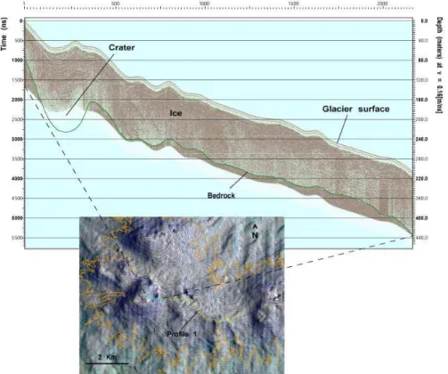
GPR profiles were processed using the software “Ground Vision”, “Reflex” and “King-dom Suite” to detect ice depth. The whole record was structured in three different files

10

(Profile 1, 2 and 3). Due to the computer configuration that limited record time window, the bedrock was sometimes too deep to be detected. However, it was possible to ex-trapolate by following ice stratifications. Whenever this was possible, such evaluations were processed. Figure 3 shows a portion of analysed Profile 1.

4.1.2 Modelling remaining ice: results

15

In order to extrapolate the estimation of the ice volume to the rest of the map, the hy-pothesis was made that the depth of ice was dependent on the altitude, the orientation (aspect) and the slopes. This follows the theory on the formation of glaciers, where the accumulation of ice is associated with wind direction, amount of precipitations and temperatures. All three depending on altitude, slopes and slope orientation (due to

20

different solar radiations). On steep slopes the ice is thinner as the glacier is moving faster, whereas on gentle slopes, the ice accumulates as the glacier slows down.

(10)

de-TCD

3, 831–856, 2009

P. Peduzzi et al.

Title Page

Tables Figures

◭ ◮

Back Close

Full Screen / Esc

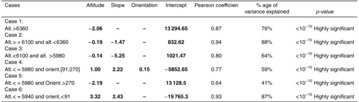
Interactive Discussion fine the ice thickness, and finally three differentiations of slope orientation were needed

for altitudes lower than 5980 (aspect higher than 270◦_{, between 91}◦ _{and 270}◦ _and

smaller than 91◦_{). Table 2 describes the variables (Altitude, slope and orientation) and}

weight (in bold) used in the model according to the different thresholds. The quality of the model was assessed by looking atp-value (all smaller than 10−10_{) and Pearson}

5

coefficient (between 0.80 and 0.94 for altitudes higher than 5980). The model becomes less accurate for lower elevations, this is reflected by a lower correlation (between 0.64 and 0.77 except one at 0.934).

Equations for Table 2 suggest that for altitudes lower than 6360 m, aspect, slopes and altitudes explain the depth of ice; while on the summit (altitude>6360) ice depth

10

is only linked with altitude. This is not surprising given that the smooth round summits of Coropuna have limited aspect variation and are mostly flat.

The map in Fig. 4 shows the result of this model once extrapolated to the entire glacier.1 The thickness ranges between 20–200 m, with an average thickness esti-mated (based on the model) between 91.6 and 95 m. If extrapolated to the whole area,

15

the volume is expected to be between 5.25 and 5.46 km3.

4.1.3 Discussion

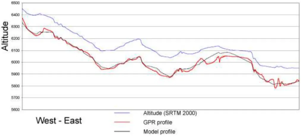
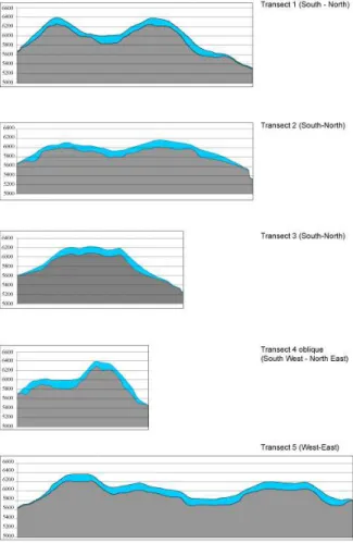
The multiple regression analysis confirmed that altitude, slopes and orientation are factors influencing the ice thickness. The quality of the model was evaluated by com-paring the measured thickness of the ice with the findings of the model (see Fig. 5).

20

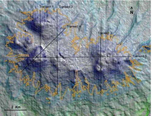
The modelled depth was found to follow the recorded profile with su_fficient precision. Figure 6 shows the location of the different transects across the model, while Fig. 7 depicts the variation of ice thickness (in blue) across the five different transects. The findings show that the ice is thicker at high altitude and on gentle slope, which is co-herent with established theory. In Transect 4, the crater of an old volcano can be seen.

25

1

(11)

TCD

3, 831–856, 2009

P. Peduzzi et al.

Title Page

Tables Figures

◭ ◮

Back Close

Full Screen / Esc

4.2 Ice volume loss

4.2.1 Findings and limitations

The accuracy of available digital elevation models remains very low. The free DEMs provided by ASTER have an accuracy of 30 m according to the USGS, who generates them. However, studies made using these DEMs, reveal significant errors when applied

5

to rugged terrain and steep slopes (K ¨a ¨ab et al., 2002). In this current analysis, errors on the rock were significant and raised concerns on the ability to use DEMs. In any cases, they could not be used without the calibration.

The “simple adjusted method” as used in Eqs. (2) and (3), was applied. An average thickness difference of 16.73 m was found by subtracting average altitude on the glacier

10

in 1955 with the same areas in 1997 (see Table 3). A difference of 10.49 m was found using the same process applied between 1955 and 2002. Although the Coropuna region received much precipitation during the El Ni ˜no 1997/98, the smaller di_fferences observed in 2002 as compared to 1997 is more likely to be due to data quality rather than linked with a 6 m increase in ice thickness between 1997 and 2002. The 1997

15

radar DEM is more precise on the rocky area, although it includes a significant amount of “no data” findings.

Figure 8, presents the loss of thickness (in red), unfortunately the radar image in-clude 24% no data readings over the study area (in black). The same computation using the ASTER DEM presented a smaller average difference, although with higher

20

variations.

The margin of error being important, it is di_fficult to guess which of the DEM di_ff er-ence is closer to the reality. According to these results the average yearly losses could vary between 0.22 and 0.4 m per year). Once extrapolated to the volume. The loss of ice between 2002 and 1955 is comprised between 1.2 and 2.1 km3. This corresponds

25

(12)

TCD

3, 831–856, 2009

P. Peduzzi et al.

Title Page

Tables Figures

◭ ◮

Back Close

Full Screen / Esc

Interactive Discussion technologies and the date of oldest archive found was 1997.

The methodology for identifying the ice volume loss using DEM is straightforward and less challenging compared to the estimation of remaining ice. The difficulty comes from the lack of precision of DEM on rough terrain. It is expected, however, that such technologies will evolves as numerous new radar sensors are now available, including

5

some with finer spatial resolution.

5 Conclusions

The methods chosen for ice thickness and ice volume loss estimation proved to be efficient, although the choice of a lighter GPR would have eased the data collection.

Using the profiles from the ground study and a statistical extrapolation (modelling)

10

it was possible to estimate the ice thickness between 91.6 and 95 m, which gives an estimated remaining volume comprise between 5.25 and 5.46 km3 (i.e. 3.68 and 3.8 millions tons of water).

The study using the DEM provided for most of the imprecision. DEM elevation ac-curacy is estimated to be+/–30 m and extensive statistical corrections were needed to

15

make them comparable. Nevertheless, it shows that the Coropuna glacier is reducing both in area and volume. The average thickness loss is estimated between 0.22 and 0.40 m per year.

It is not possible with the current number of DEMs to say if the loss is linear or if it will accelerate. To assess this, new measures would need to be taken, every 4–5 years. It

20

is recommended to use radar satellite images. The more expensive radar DEM proved to be more accurate than ASTER passive sensors. If DEM are taken every five years or so, within 15 years it should be possible to say if the ice reduction is linear or is accelerating.

In order to avoid the risk of including snow cover in the estimates data should be

25

(13)

TCD

3, 831–856, 2009

P. Peduzzi et al.

Title Page

Tables Figures

◭ ◮

Back Close

Full Screen / Esc

Interactive Discussion The results from this study were presented to GTZ and UNDP. Although the ice

vol-ume loss was strongly suspected, having factual numbers to present to these develop-ment agencies, helped to convince them to continue supporting research and irrigation projects. A follow-up study for evaluating the impacts on water supply, might consist in assessing where the most important water sources are located and how they might be

5

impacted by the glacier retreat. A precise delimitation of water catchments, measure of river flows at different places are tools that would allow a refined planning for future irrigation of crops.

Acknowledgements. This work was supported by the GTZ/COPASA, Arequipa. We would like

to thanks Josef Haider, Juan Carlos Montero and all the team of GTZ/COPASA in Arequipa

10

for the logistical support and for trusting us in conducting this study. We also would like to thanks Carlos Zarate and all his team for the expedition on Coropuna, and the team of Peruvian Geophysical Institute in Arequipa. Without all these supports this research would not have been possible. For the help provided in seismic and GPR data acquisition and analysis, we would like to thanks Milan Beres, Julien Fiore and Micha ¨el Fuchs of Department of Geology, University

15

of Geneva, Jacques Jenny of Geo2x, Franc¸ois Marillier and Dieb Hammami of Geophysical Institute, University of Lausanne, and Ansgar Forsgren of Mala Geoscience. We also would like to thank John Harding for his editing suggestions.

References

Bates, B. C.: Climate Change and Water, edited by: Kundzewicz,Z. W., Wu, S., and Palutikof, J.

20

P., in: Technical Paper of the Intergovernmental Panel on Climate Change, IPCC Secretariat, Geneva, online available at: http://www.hm-treasury.gov.uk/stern review report.htm, 210 pp., 2008.

Eisen, O., Nixdorf, U., Keck, L., and Wagenbach, D.: Alpine ice cores and ground pen-etrating radar: combined investigations for glaciological and climatic interpretations of a

25

cold Alpine ice body, online available at: http://epic.awi.de/epic/Main?puid₌ 16358,Alfred-Wegener-Institut f ür Polar- und Meeresforschung Bremerhaven, Institut f ür Umweltphysik, Universit ät Heidelberg, 2003.

(14)

TCD

3, 831–856, 2009

P. Peduzzi et al.

Title Page Abstract Introduction Conclusions References Tables Figures ◭ ◮ ◭ ◮ Back Close

Full Screen / Esc

Interactive Discussion Glaciology and Permafrost Prospecting, online available at:http://www.sgruber.de/pap-rad.

htmGeographischesInstitut/JLUGiessen, 1996.

K ¨a ¨ab, A., Huggel, C., Paul, F., Wessels, R., Raup, B., Kiefer, H. and Kargel, J.: Glacier Mon-itoring from ASTER imagery: accuracy and applications, Proceedings of EARSeL-LISSIG-Workshop Observing our Cryosphere from Space, Bern, Switzerland, 2002.

5

Maijala, P., Moore, J. C., Hjelt, S. E., P ¨alli, A., and Sinisalo, A.: GPR Investigations of Glaciers and Sea Ice in the Scandinavian Arctic, GPR98 – 7th International Conference on Ground-Penetrating Radar Proceedings., online available at: http://www.ulapland.fi/home/hkunta/ jmoore/johnarticles.html 143–148, 1998.

Racoviteanu, A. E., Manley, W., Arnaud, Y., Williams, M. W.: Evaluating digital elevation models

10

for glaciologic applications: an example from Nevado Coropuna, Peruvian Andes. Global Planet. Change, 59(1–4), 110–125, 2007.

Snchal, G., Rousset D., Salom A.-L., and Grasso J.-R.: Georadar and seismic investigations over the Glacier de la Girose (French Alps), Near Surface Geophysics 1, 5–12, 2003. Silverio, W.: Cartografia multi-temporal de la cobertura glaciar de nevado Coropuna (6425 m)

15

entre 1955 y 2003, report to GTZ/COPASA, 2005.

Silverio, W.: An álisis de los par ámetros clim áticos de las estaciones en la regi ón del Nevado Coropuna (6425 m. s. n. m.), Arequipa, Per ú. Informe preparado para la GTZ-Arequipa-PERU (COPASA), Documento interno, 2005b.

Silverio, W. and Jaquet, J. M.: Glacial cover mapping (1987–1996) of the Cordillera Blanca

20

(Peru) using satellite imagery, Remote Sens. Environ., 95(3), 342–350, 2005.

Stern, N.: The Stern Review Report: the Economics of Climate Change, London, HM Treasury, 30 October 2006, online available at: http://www.hm-treasury.gov.uk/stern review report. html, 603, 2006.

Vimeux, F., Ginot, P., Schwikowski, M., Vuille, M., Hoffmann, G., Thompson, L. G., and

Schot-25

tererg, U.: Climate variability during the last 1000 years inferred from Andean ice cores: A review of methodology and recent results, Palaeogeogr., Palaeocl., in press, 2009.

Vuille, M., Francou, B., Wagnon P., Juen, I., Kaser, G., Bryan G. M., and Bradley, R. S.: Climate change and tropical Andean glaciers: Past, present and future, Earth Sci. Rev. 89, 79–96, 2008.

30

(15)

TCD

3, 831–856, 2009

P. Peduzzi et al.

Title Page

Tables Figures

◭ ◮

Back Close

Full Screen / Esc

Table 1.Data sources for DEM.

DEM Year Origin Resolution No data

DEM 1955 1955 Topographic map 30 m 0%

DEM 1997 Oct 1997 ESA/ERS 25 m 24%

DEM 2000a Feb 2000 NASA/SRTM 90 m 0% (corrected)

DEM 2000b Oct 2000 NASA/ASTER 30 m 0%

DEM 2001 Jul 2001 NASA/ASTER 30 m 0%

DEM 2002a May 2002 NASA/ASTER 30 m 0%

DEM 2002b Nov 2002 NASA/ASTER 30 m 0%

(16)

TCD

3, 831–856, 2009

P. Peduzzi et al.

Title Page

Tables Figures

◭ ◮

Back Close

Full Screen / Esc

Table 2.Settings of parameters for the GPR.

Record parameters Settings

Sampling frequency 438 MHz Number of samples 900 Number of stacks 16

Time window 2055 ns

(17)

TCD

3, 831–856, 2009

P. Peduzzi et al.

Title Page

Tables Figures

◭ ◮

Back Close

Full Screen / Esc

Table 3.Quality of regressions used for modelling ice thickness.

Cases Altitude Slope Orientation Intercept Pearson coefficien % age of

variance explained p-value Case 1:

Alt.>6360 −2.06 – – 13 294.65 0.87 76% <10−10Highly significant

Case 2:

Alt.>=6100 and alt.<6360 −0.19 −1.47 – 832.62 0.94 88% <10−10Highly significant

Case 3:

Alt.<6100 and alt.>5980 −0.14 −5.25 – 1021.47 0.80 64% <10−10Highly significant

Case 4:

Alt.<=5980 and orient.[91;270] 1.00 2.22 0.15 −5852.65 0.77 59% <10−10Highly significant

Case 5:

Alt.<=5980 and Orient.>270 −2.19 – – 13 128.5 0.64 41% <10−10Highly significant

Case 6:

Alt.<=5940 and orient.<91 3.32 2.43 – −19 765.3 0.93 87% <10−10

(18)

TCD

3, 831–856, 2009

P. Peduzzi et al.

Title Page

Tables Figures

◭ ◮

Back Close

Full Screen / Esc

Table 4.Computation of ice di_fference using adjusted di_fference.

DEM Rock Ice Diff. Rock Diff. Ice Adj. Diff.

1955 (Map) 4776.90 5543.47 0.00 0.00 0.00

1997 (Radar) 4769.14 5518.99 7.75 24.48 16.73

2002b (ASTER) 4823.27 5579.35 ₋46.38 ₋35.88 10.49

(19)

TCD

3, 831–856, 2009

P. Peduzzi et al.

Title Page

Tables Figures

◭ ◮

Back Close

Full Screen / Esc

(20)

TCD

3, 831–856, 2009

P. Peduzzi et al.

Title Page

Tables Figures

◭ ◮

Back Close

Full Screen / Esc

(21)

TCD

3, 831–856, 2009

P. Peduzzi et al.

Title Page

Tables Figures

◭ ◮

Back Close

Full Screen / Esc

(22)

TCD

3, 831–856, 2009

P. Peduzzi et al.

Title Page

Tables Figures

◭ ◮

Back Close

Full Screen / Esc

(23)

TCD

3, 831–856, 2009

P. Peduzzi et al.

Title Page

Tables Figures

◭ ◮

Back Close

Full Screen / Esc

(24)

TCD

3, 831–856, 2009

P. Peduzzi et al.

Title Page

Tables Figures

◭ ◮

Back Close

Full Screen / Esc

(25)

TCD

3, 831–856, 2009

P. Peduzzi et al.

Title Page

Tables Figures

◭ ◮

Back Close

Full Screen / Esc

(26)

TCD

3, 831–856, 2009

P. Peduzzi et al.

Title Page

Tables Figures

◭ ◮

Back Close

Full Screen / Esc