Visualising Pipeline Sensor Datasets with Modified Incremental
Orthogonal Centroid Algorithm
Olufemi Ayinde Folorunso1 and Shahrizal Sunar Mohd2
1
UTMViCubeLab,
Department of Computer Graphics & Multimedia, Faculty of Computer Science and Information Systems,
Universiti Teknologi Malaysia, 81310, Skudai, Johor
2
UTMViCubeLab,
Department of Computer Graphics & Multimedia, Faculty of Computer Science and Information Systems,
Universiti Teknologi Malaysia, 81310, Skudai, Johor
Abstract
Each year, millions of people suffer from after-effects of pipeline leakages, spills, and eruptions. Leakages Detection Systems (LDS) are often used to understand and analyse these phenomena but unfortunately could not offer complete solution to reducing the scale of the problem. One recent approach was to collect datasets from these pipeline sensors and analyse offline, the approach yielded questionable results due to vast nature of the datasets. These datasets together with the necessity for powerful exploration tools made most pipelines operating companies “data rich but information poor”. Researchers have therefore identified problem of dimensional reduction for pipeline sensor datasets as a major research issue. Hence, systematic gap filling data mining development approaches are required to transform data “tombs” into “golden nuggets” of knowledge. This paper proposes an algorithm for this purpose based on the Incremental Orthogonal Centroid (IOC). Search time for specific data patterns may be enhanced using this algorithm
Keywords: Piggin, Heuristics, Incremental, Centroid.
1. Introduction
Pipelines are essential components of the energy supply chain and the monitoring of their integrities have become major tasks for the pipeline management and control systems. Nowadays pipelines are being laid over very long distances in remote areas affected by landslides and harsh environmental conditions where soil texture that changes between different weathers increase the probability of hazards not to mention the possibility of third party intrusion such as vandalism and deliberate attempt of diversions of pipeline products. It is widely accepted that leakages from pipelines have huge environmental, cost and image impacts.
Conventional monitoring techniques such as the LDSs could neither offer continuous pipeline monitoring over the whole pipeline distance nor present the required sensitivity for pipeline leakages or ground movement detection. Leakages can have various causes, including excessive deformations caused by earthquakes, landslides, corrosion, fatigue, material flaws or even intentional or malicious damaging.
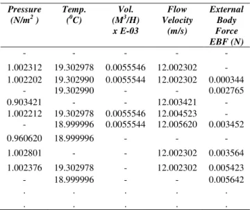
Table 1: Data Attributes and Variables from the Velocity-Vane Anemometer
Even if every pixel on a standard display device is used to represent each datum, display device with the best resolution cannot display all the data generated by theses sensors in 1 minute at the same time, not even the 53 million pixel power wall presently being used at the University of Leeds [1]. The same goes for the memory size that is required for such computation as well as the computational time. Definitely, this will of course require greater computational effort and some compromises of visualisation results. Hence, users of visualisation applications tend to rely heavily on heuristics to arriving at decisions from their applications. Dimensionality reduction is therefore an alternative technique to explaining and understanding these vast pipeline sensors datasets more intuitively. Presence or absence of leakages or abnormal situations is gradually becoming the object of research in the recent time. In Nigeria, the 1992 pipeline explosions that claimed thousands of lives in Ejigbo is one good example of such underground oil installations that resulted to explosions and allied problems as a result of undetected leakage and bad response time to leakages due to imperfection and the errors in the visualisation and LDS systems. The mayhem was traced to inability to properly analyse and visualise leakage points about the pipeline. Although most of these pipeline failures are blamed on the activities of the vandals especially in developing nations, yet, the basic truth is that the visualisations of the various leakage detection systems are error-full. When leakages are quickly detected and fixed, it invariably reduces the vandals’ activities as well as saving lives and reducing the overhead installation and administrative costs associated with pipeline installation and pigging operations.
A central problem in scientific visualisation is to develop an acceptable and resources efficient representation for such complex datasets [2, 3]. The challenges of high dimensional datasets vary significantly across many factors and fields. Some researchers including [4] and [5] viewed these challenges as scientifically significant for positive theoretical developments. There are so many problems of high dimensional datasets ranging from attributes relevance and presence to variable importance. In practical sense, not all the dimensions or attributes and not all variables or instances- presence or absence in high dimensional datasets are relevant for every specific user defined interests in understanding certain underlying phenomena represented by the datasets.
More recently, [5, 6, and 7] asserted that principal among the problems of dimensionality reduction is the issue of accuracy compromise. They all submitted that almost all data reduction algorithms and methods employ one or more procedures that lead to significant compromise of accuracy. Without any loss of generality, the problem under investigation has to do with trying to find the extent of allowable and reasonable reduction in data dimensions that could be carried out on high pipeline sensor datasets without a compromise of the desired visualisation quality obtainable from such datasets under specific or desired boundary conditions. Mathematically, given an n-dimensional random variable x = (x1, … . xn)T
a lower dimensional random variable s = (s1, … . sm)T
with n >>> m such that the entire member data of x are
fully represented by s with n , m Є R (R is the set of real
numbers) is required. The overall goal of reducing the data dimension is to enable a lower dimensional space reveal to us “as much as possible” details about a high dimensional data space with minimal loss of data integrity and compromise.
Often in computer graphics this is very necessary because the available devices (such as monitors) cannot display all the intrinsic elements of the voluminous datasets generated by modern day sensors and remote sensing devices. If the dimensionality of datasets could be reduced, the resulting data could be used more effectively in visualisation, verification, classification, and exploration. There are many dimensionality reduction algorithms and approaches. These are discussed in Section 2 of this paper.
Pressure (N/m2 )
Temp. (0C)
Vol. (M3/H) x E-03
Flow Velocity
(m/s)
External Body Force EBF (N)
- - - - -
1.002312 19.302978 0.0055546 12.002302 - 1.002202 19.302990 0.0055544 12.002302 0.000344
- 19.302990 - - 0.002765
0.903421 - - 12.003421 -
1.002212 19.302978 0.0055546 12.004523 - - 18.999996 0.0055544 12.005620 0.003452
0.960620 18.999996 - - -
1.002801 - - 12.002302 0.003564
1.002376 19.302978 - 12.002302 0.005423
- 18.999996 - - 0.005642
. . . . .
2. Literature Review
Reducing dimensionality has been described as an essential task for many large-scale information processing problems involving document classification, searching over Web data sets [5]. Because of the exponential growth of the Web information and other remote sensing devices, many traditional classification techniques now require a very huge amount of memory and CPU resource if dimensionality reductions are not performed on the datasets as required. Sometimes, dimensionality reduction is a pre-processing step in data mining but may also be some steps towards data exploration and analysis such as in data clustering, visualisation etc. Historically, the Principal Components Analysis (PCA) originally credited to Pearson (1901) whose first appearance in modern literatures dates back to the work by Hotelling (1933) was a popular approach to reducing dimensionality. It was formerly called the Karhunen-Loeve procedure, eigenvector analysis and empirical orthogonal functions. The PCA is a linear technique that regards a component as linear combinations of the original variables . The goal of PCA is to find a subspace whose basis vectors correspond to the directions with maximal variances.
Let X be an dxp matrix obtained from sensor datasets for example, where d represents the individual data attributes (columns) and p the observations (or variables) that is being measured. Let us further denote the covariance matrix C that defined X explicitly as:
C =1
n∑ (xi−x�)(xi−x�) T n
i=1 (1.0)
Where xi Є X and x� is the mean of xi , T is the
positional order of xiЄ X, and X is the covariance matrix
of the sampled data. We can thus define an objective function as:
G(w) = WTCW (2.0)
The PCA’s aims is to maximise this stated objective function G(W) in a solution space defined by:
Hdxp =�WЄ Rdxp, WTW = I� (3.0)
It has been proved that the column vectors of W are the p higher or maxima eigenvectors of covariance matrix C defined above [see 8]). However, for very large and massive datasets like the pipeline sensors datasets, an enhancement of the PCA called the Incremental PCA developed by [9,10] could be a useful approach. The IPCA is an incremental learning algorithm with many variations. The variations differ by their ways of incrementing the internal representations of the covariance matrix. Although
both the PCA and the IPCAs are very effective for most data mining applications, but, because they ignore the valuable class label information in the entire data space, they are inapplicable for sensor datasets.
The Linear Discriminant Analysis (LDA) emerged as another approach commonly used to carry out dimensionality reduction. Its background could be traced to the PCA and it works by discriminating samples in their different classes. Its goal is to maximize the Fisher criterion specified by the objective function:
�(�) =�������
������� (4.0)
Where sb=∑c pi(mi−�x)(mi−x�)T
i=1 and sw =
∑ci=1pi E((x−mi)(x−mi)T} with x Є ci are called the
Inter class scatter matrix and Intra class scatter matrix respectively. E denotes the expectation and pi(x) =
ni
n is
the prior probability of a variable (x) belonging to attribute (i).
W can therefore be computed by solving w∗= arg max G(w) in the solution space Hdxp =�WЄ Rdxp, WTW = I�, in most reports; this is
always accomplished by providing solution to the generalized eigenvalue decomposition problem represented by the equation:
Sbw =λSww (5.0)
When the captured data is very large like in the case of sensors datasets considered in this research, LDA becomes inapplicable because it is harder and computationally expensive to determine the Singular Value Decomposition (SVD) of the covariance matrix more efficiently. LDA uses attribute label information of the samples, which has been found unsuitable by many researchers including [5] for numerical datasets. [11] had developed a variant of the LDA called the Incremental LDA (ILDA) to solve the problem of inability to handle massive datasets, but, its stability for this kind of application remains an issue till present date.
decomposition are too expensive for large-scale data such as Web documents. Further, its application to numerical data or multivariate and multidimensional datasets of this sort remains a research challenge till date. However, its basic assumptions are extremely acceptable for development of such better algorithms.
In 2006, a highly scalable incremental algorithm based on the OC algorithm called the Incremental OC (IOC) was proposed by [5]. Because OC largely depends on the PCA, it is therefore not out of focus to state that the IOC is also a relaxed version of the conventional PCA. IOC is a one-pass algorithm. As dimensionality increases and defiles batch algorithms, IOC becomes an immediate alternative. The increase in data dimensionality could now be treated as a continuous stream of datasets similar to those obtainable from the velocity vane thermo-anemometer (VVTA) sensors and other data capturing devices, and then we can compute the low dimensional representation from the samples given, one at a time with user defined selection criterion Area of Interest (AOI) (iteratively). This reassures that the IOC is able to handle extremely large datasets. However, because of its neglect of the variables with extremely low eigenvalues, it is poised to be insensitive to outliers. Unfortunately, this is the case with the kind of data used in this research. There is therefore a necessity to improve the IOC algorithm to accommodate the insurgencies and the peculiarity presented by pipeline sensor datasets. The derivation of the IOC algorithm as well as the improvement proposed to the algorithm is discussed in detail in the following subsections.
3. IOC Derivation and the Proposed (HPDR)
Improvement
Basic Assumption 1: The IOC optimization problem could be restated as
max ∑ WTS bW p
i=1 (6.0)
The aim of this is to optimise equation 6.0 with W Є Xdxp
, where the parameters have their usual meanings. However, this is conditional upon wiwiT=1 with i=1,2,3,….p. Now, p
belongs to the infinitely defined subspace of X, but, since it is not possible to select the entire variables for a particular data attribute at a time, we introduced a bias called Area of Interest (AOI) to limit each selection from the entire data space.
A Lagrange function L is then introduced such that: L(wk,λk) =∑ wkSbwkT
p
i=1 − λk(wkwkT−1)
Or
L(wk,λk) =∑ wkSbwkT p
i=1 − λkwkwkT+λk) (7.0)
(Observe that if wkwkT=1, then equation (7.0) is
identically (6.0))
With λk being the Lagrange multipliers, at the saddle
point, L must = 0. Therefore, it means SbwkT =λkwkT
necessarily. Since obviously p >>>AOI at any point in time, this means that, w, the columns or attributes of W are p leading vectors of Sb. Sb (n) Can be computed therefore
by using:
Sb(n) =∑AOIpj(n)
j=1 (mj(n)−m(n))(mj(n)−m(n))T
(8.0)
Where mj(n) is the mean of data attribute j at step i and m(i) is the mean of variables at step i. T is the order of the variable in the covariance matrix defined by data space X. To dance around this problem, the Eigen Value Decomposition (EVD) is the approach that is commonly used although it has been reported to have high computation complexity problems.
The EVD is computed by following the following procedure:
Given any finite data samples X={x1,x2,x3,...,xn} we first
compute the mean of xi by using the conventional
formula:
μ=1
n∑ xi n
1 (9.0)
This is followed by the computation of the covariance C defined as:
C =1
n∑ (xi− n
1 x�)(xi−x�)T (10.0)
Next, we compute the eigenvalue λ(s) and eigenvectors e(s) of the matrix C and iteratively solve:
Ce=λe (11.0) PCA then orders λ by their magnitudes such that λ1
>λ2>λ3>... >λn , and reduces the dimensionality by keeping direction e such that λ <<< T. In other words, the
PCA works by ignoring data values whose eigenvalue(s) seems very insignificant. To apply this or make it usable for pipeline sensor datasets, we need a more adaptive incremental algorithm, to find the p leading eigenvectors of Sb in an iterative way. For sensor datasets, we present
each sample of the selected AOI as: (x{n}, ln) where x{n}
is the nth training data, ln is its corresponding attribute
Basic Assumption 2: if given limn→∞a(n) = a, then limn→∞(
1
n∑ a(i)) = a n
i=1 by induction, therefore, it means
that limn→∞sb(n) = sb, using Assumption 1.0: which
means that:
limn→∞(1n∑ni=1sb(�)) = sb (12.0)
However, the general eigenvector form is Au =λu,
where u is the eigenvector of A corresponding to the eigenvalue-λ. By replacing the matrix A with sb(n), we can obtain an approximate iterative eigenvector
computation formulation with v = Au =λu or u= v/λ:
v(n) = 1
n∑ sb(i) u(i) n
i=1 (13.0)
Injecting equation 8.0 into equation 13.0 implies: v(n) = 1
n� �pj(n)
AOI
j=1
(mj(n) n
i=1
−m(n))(mj(n)−m(n))T u(i)
Assuming that Φj(i)= mj(n)−m(n); it means
v(n) = 1
n∑ ∑ pj(n) AOI
j=1 Φj(i)Φj(i)T u(i) n
i=1 (14.0)
Therefore, since u= v/λ: the eigenvector u�⃗ can be computed using
u �⃗= v
‖v‖ (15.0)
But, vector u�⃗(i) could be explicitly defined as u
�⃗(i)= v(i−1)
‖v(i−1)‖ , with i=1,2,3,…n. Therefore,
v(n) = 1
n∑ ∑ �pj(n)Φj(i)Φj(i) T� AOI
j=1
v(i−1) ‖v(i−1)‖ n
i=1 (16.0)
Hence; v(n) =
n−1
n v(n−1) + 1
n∑ �pj(n)Φj(n)Φj(n) T� AOI
j=1
v(n−1)
‖v(n−1)‖
(17.0) If we substitute ξj(n) = Φj(n)T v(n−
1)
‖v(n−1)‖ ,
j=1,2,3….AOI, and if we set v(0)=x(1) as a starting point, then it is comfortable to write v(n) as:
v(n) = v(n−1) 2
n +
1
n∑ �pj(n)Φj(n) ξj(n)� AOI
j=1 (18.0)
Since the eigenvectors must be orthogonal to each other by definition. Therefore, we could span variables in a complementary space for computation of the higher order eigenvectors of the underlying covariance matrix. To
compute the (j+α)th eigenvector, where α=1,2,3…AOI, we
then subtract its projection on the estimated jth eigenvector from the data.
��+�(�) =��(�)−(��(�)���(�))
���(�)�2 (19.0) (Note that j+α = AOI for any particular selection)
Where x1(n)= x(n). Using this approach, we have been
able to address the problem of high time consumption. This is because the orthogonality could now only be enforced when there is convergence which may not be at the beginning but may occur at any point at the extreme end of the selected and repeated AOIs. Through the projection procedure at each step, we can then get the eigenvectors of Sb one by one (i.e for each set of the
predetermined AOI). The IOC algorithm summary as presented by [5] is shown in Algorithm 1 and improved IOC called the HPDR algorithm is presented in Algorithm 2.0, the solution of step n is given as:
vj(n) = vj(n)
�vj(n)� with j=1,2,3…p (20.0)
3.1The IOC Algorithm and the HPDR
By going through the algorithm an example could be used to illustrate how HPDR solves the leading eigenvectors of Sb incrementally and sequentially. Let us assume that
input sensor datasets obtained from the two sources (manually and experimentally) are represented by {ai },
i= 1,2,3,… and {bi }, i= 1,2,3… When there is no data
input, the means m(0), m1(0), m2(0), are all zero. If we let
the initial eigenvector v1(1) =a
1 for a start, then HPDR
algorithm can be used to compute the initial values or the leading samples of the datasets ai(s) and bi(s) of the entire
data space X. These initial values are given as: a1, a2, and
b1, b2, and they can then be computed using equation 20.0.
3.2 The Expected Likelihoods (EL)
Given an arbitrary unordered set of data X defined by X={x1,x2,x3,…xn }k along with a set of unordered
attributes Z={X1,X2,X3,…XN}k-n such that the attitudinal
vector Zψ depends on the covariance matrix or X . The rowsum (RS), columsum (CS) and Grandtotal (GT) of the
covariance matrix X│Xψ are defined as:
RS =∑ki=1{Xi}N (21.0)
CS =∑ki=1−n{Zi}N (22.0)
And
GT =∑i=1k−n{Zi}N+∑ki=1{Xi}N (23.0)
Using the product of the respective Row Sum (RS) the Column Sum (CS) divided by the Ground Total (GT), the expected for each of the covariance matrix elements could be estimated. The computation begins with the initialisation of counters for the row, the column and the Area of Interest (AOI) selected as i , j, and N respectively. The datum in the first data value in the first row and the first column is read and the expected value for this position is computed. The jth column positional value is advanced until all the five dimensions (J=5) are all traversed. The system then increment i and moves to the (i+1)th row positional value and the process continues until the entire value of the AOI=N is completely traversed. The WAEL is thus computed by finding the weighted average value of the data attributes as shown in Algorithm 2.0. Thus, the expected variable xi of {X} belonging to position {xi,yi} of the covariance matrix X is computed using the expected likelihood function:
Ek(xi, yi) = RS +CS
GT (24.0)
The Averaged Expected Likelihood Al for Ek(xi, yi) is
defined further by
Al =
�Ek k−n
k=1
�
Ek−n → on major axis .
.
0 elsewhere
� (25.0)
This gives a unit dimensional matrix A representing the original data X.
3.3 Weighted Average Expected Likelihoods
(WAEL)
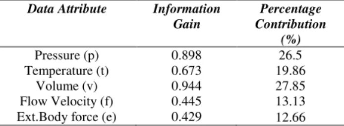
The WAEL is the weighted mean of the expected likelihoods and it is comparable but not the same as the arithmetic mean. It is based on the assumption that although each data value is important, they do not contribute equally to the flow dynamics and the selected datasets. It is determined by computing the average for the reduced expected likelihoods with a weight factor for each data entity. The weight factor (or the Information Gain (IG)) is the degree of sensitivity of the attribute to the entire data space. This idea plays a role in descriptive statistics and it also occurs in more general forms other areas of statistics and mathematics. This position is justified because judging from the IG computation for each of the attributes; we could see that each of the sensor data attributes contributes differently to the entire flow process. It will therefore be very illogical to use the simple average for the computation of the likelihoods.
Although WAEL will behave similar to the normal statistical means, if all the sensor datasets are equally weighted, then what is computed is just the arithmetic mean which is considered unsuitable for sensor datasets due to its variability. Example of such effects is found in what the statisticians know as the Simpson’s Paradox. This paradox illustrates how correlation in different groups of data is completely reversed by just combining the two data groups. This is always the case when frequency of data is given causal interpretations hastily. However, Simpson’s Paradox will disappear if causal relations (in terms of frequencies) are brought into consideration. The computation follows the conventional weighted average formula for the reduced dimension. For example in Table 2. we expanded IG computation for datasets represented in Table 1. to reflect the percentage contributions of each attributes. The percentage contribution is then calculated by the formula %Contribution = (Gain/Total Gain)*100.
Table 2: Percentage Contributions of Attributes Data Attribute Information
Gain
Percentage Contribution
(%)
Pressure (p) 0.898 26.5
Temperature (t) 0.673 19.86
Volume (v) 0.944 27.85
3.4 Data Attributes Selection
Based on the generated metadata, the data attributes selection could be performed by using the modified back propagation algorithm. Without modification, back propagation algorithm lacks robustness this is because errors grow exponentially while the attribute weight diminishes. It is observed that as the bias increases, there is heavy tendency for the error inherited into the visualisation to also rise. In the conventional back propagation algorithm, each attribute is given a weight which equals the sum of the errors inherited multiplied by the mean data entity. This condition of the back propagation algorithm has greatly mediated its use for modern applications of this sort.
With this modification however, it is possible to reduce the errors inherited by inversing the error threshold as shown in the modified version in Section 4. There are alternative methods for carrying out data classification, however, due to its robustness and wider acceptability, the decision tree algorithm by [15] is employed to carry out data classification. This algorithm works by computing the Information Gain (I.G) for each data attribute and promoting the one with the highest gain as the root for the tree as the test or lead attribute. This method forces the lead attribute to “inherit” transferable qualities of the other attributes which in turn provided a basis for quicker visualisation. The computation of the IG is achieved by using the conventional information gain formula:
I(s1, s2, … sm) =− ∑mi=1pilog2(pi) (26.0)
Where pi = si/s is the probability that an arbitrary sensor data belong to a class Ci . Log base 2 has been used because the data are encoded in bits and si is the number of sample S in class Ci. m is the number of case attributes.
3.5 High Performance Dimensionality Reduction
Algorithm (HPDR)
To achieve high performance in dimensionality reduction, this paper is structured as a form of combinational framework (like a bridge) between the Feature Extraction based method -IOC and the Feature Selection based method- the EL. The strength is derived by the introduction of a mechanism for users’ choice of Areas of Interest (AOI). This is made possible by effectively determining the IG by each of the attributes and determining the lead attribute. Fixing the expected likelihood for the cases of emptiness completely remove the shortfalls insensitivity to outliers and less significant variables in the dataset [16]. Using this approach is not completely new; it has been found extremely advantageous in statistical and mathematical applications see examples
in [17, 18 19]. It is often used for the computation of the popular Chi-square in non-parametric statistics for example. The normalised data is simply subjected to the HPDR (Algorithm 2).
Algorithm 1: Conventional IOC Dimensionality Reduction Algorithm
*Yan et al.(2006)
Dimensionality reduction algorithms are extremely useful in improving the efficiency and the effectiveness of datasets classifiers [5]. Reducing dimensionality this way is of great importance to ensure quality and efficiency of data classifiers for large scale and continuous data streams like sensor’s datasets, this is because of the poor classification efficiency of earlier approach such as the IOC powered by the high dimension of the data space. It has been viewed and described as an essential data mining and data pre-processing approach for large scale and streaming datasets classification tasks.
3.6 Analysing the HPDR Algorithm
for n=1,2,3,…AOI do the following steps:
M(n)=((n-1)m(n-1)+x(n))/n
Nln(n)= Nln(n-1)+1
Mln(n)=(Nln(n-1)mln(n-1)+x(n))/Nln(n)
Φi1 (n)=mi(n)-m(n), i=1,2,…5
for i=1,2,…5; j=1,2,3,… AOI (max i=5, because we have just 5 dimensions)
If j=n then Vj(n)=x(n)
else
���(�) = ���(�)� ��(�−1)
���(�−1)�
10Compute the expected E(i)for each j of the AOI Є C
Ex into position Pi;
n--
if n>1, then i++;
If i>5, j++; go to Step 10 otherwise;
Compute Weighted Averaged
Expected Likelihood (WAEL)-Al
end if
end if
Return Al into position pi
end if
end for
end for
��(�) = ��(� −1)2
� +
1
�� ���(�)��(�) ���(�)� ���
�=1
��+�(�) =� ��(�)−
(���(�)���(�)) ‖��(�)‖2
��=��� ∗ �����
�� =� � ∗ ��/5 �
�=1
αi j
(n), with i = 1,2,3, … AOI
(α (n) has its usual meaning)
Algorithm 2. High Performance Dimensionality Reduction Algorithm
When computational complexities are out of it, HPDR offers a faster approach to reducing the dimensionality of the datasets based on the predefined criteria. The strength of this algorithm lies in the interaction with subtlety of the intrinsic data interdependencies. When users are empowered to make their choice of the area to visualise or explore, better results are obtained. Because the computation is done one after the other in an iterative manner, HPDR offers the advantage of improved memory usage, this is a good and better promise that the earlier approaches in terms of the storage requirements. Viewing from another angle, considering the volume and nature of the pipeline sensor datasets, it is practically impossible to render the whole data, even after the dimensionality has been reduced. The HPDR offers the benefit of AOI selection; this enables step by step and continuous processing of the data in a manner that supersedes the conventional batch processing technique.
4. Procedures
Given D = n x m data space and two disjointed datasets
{X, Sk Є D}Assuming that dataset (X)= {xi; 1 ≤ i ≤ �Є N+} and dataset (Sk) = { sj; 1 ≤ j ≤ �Є N+} Є D such that X∩ Sk = ф, then X and Sk are independent
variables (vectors) of the set D it follows that:
Centroid (cXi) = X�+ Sk���=� 1 λ∑λj=1sj+
1 ξ∑Ii =1xi
2 � (27.0)
or 2cXi =1
λ∑λj=1sj+ 1
ξ∑ξi=1xi (28.0)
X� and Sk���� denotes the means of X and Sk respectively, � and � are arbitrary constants. If all missing �sand �s can be computed and inserted by “any means” into D such that n� = n�, it follows that:
cXi = 1
2λ�∑ sj λ
j=1 + ∑λi=1xi� (29.0)
If Sk represents a specific scenario Ap Є D. Therefore with the new centres for each classes or attributes, dataset D can be regrouped more effectively.
5. Results and Evaluation
techniques which has made comparison extremely difficult. Examples of such area or domain specific application are found in [3, 5, 6, 7, 16,17, 18, 19,20, 21, 22, 23, 24, 25, 26, 27, 28, 29, 30, 31, 32, and 33] to mention but a few.
Most researchers make use of statistical illustrations and comparative graphs to compare dimensionality reduction and data mining techniques. Examples are found in [5,16]. Dimensionality reduction helps to make better statistical decisions that could lead to significant and concrete results in pipeline sensors data visualisations. This could be in the form of increased income or energising efficient processes. The future suggests that the choice of such an effective dimensionality reduction and data mining tool will depend on the expected return on the overall efforts put into it. It is therefore imperative to critically examine and assess the overall business situation in question and how the selected tool could effectively
achieve the goals of dimensionality reduction and the data mining process. To help evaluation, some checklists have been compiled using the Cross Industry Standard Process for Data Mining (CRISP-DM).
The CRISP-DM is a six-phase process. The choice of tool however should be flexible thereby allowing selective changes to the entire data space as may be deemed necessary. The six stages involved are: Business understanding; Data understanding; Data preparation; Modelling; Evaluation and Deployment. The algorithms compared are the Principal Component Analysis (PCA), the Linear Discriminant Analysis (LDA), the Incremental Orthogonal Centroid (IOC) and the proposed High Performance Dimensionality Reduction algorithm (HPDR) on the datasets obtained from two source: The VVTA and the Turbulence Rheometer. The results obtained are presented in Table 3.
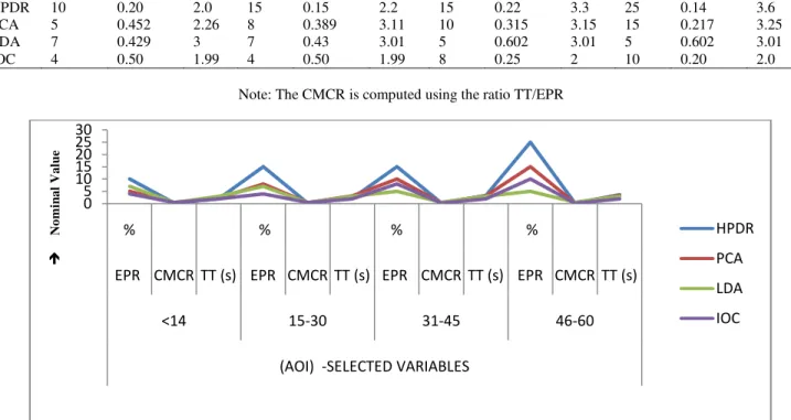
Table 3: Summary of the Result Obtained Comparing Four Dimensionality Reduction Algorithms
Note: The CMCR is computed using the ratio TT/EPR
Fig. 1. Comparing Dimensionality Reduction Algorithms The evaluation of the proposed method is designed as
an assessment of the model proposed prior deployment when compared with existing and previously used techniques. The evaluation phase examines how the
original data obtained from the sensors have been injected into the developed algorithm and how the results obtained is of any significance to the users of the system. However, this paper has been able to compare the dimensionality
0 5 10 15 20 25 30
% % % %
EPR CMCR TT (s) EPR CMCR TT (s) EPR CMCR TT (s) EPR CMCR TT (s)
<14 15-30 31-45 46-60
(AOI) -SELECTED VARIABLES
HPDR
PCA
LDA
IOC
(AOI) - SELECTED VARIABLES
<14 15-30 31-45 46-60
EPR
% CMCR
TT (s)
EPR
% CMCR TT (s) EPR
% CMCR
TT (s)
EPR
% CMCR TT (s)
HPDR 10 0.20 2.0 15 0.15 2.2 15 0.22 3.3 25 0.14 3.6
PCA 5 0.452 2.26 8 0.389 3.11 10 0.315 3.15 15 0.217 3.25
LDA 7 0.429 3 7 0.43 3.01 5 0.602 3.01 5 0.602 3.01
IOC 4 0.50 1.99 4 0.50 1.99 8 0.25 2 10 0.20 2.0
N
o
m
in
a
l V
a
lu
reduction algorithms’ efficiency when applied to reducing a five dimensional sensor data obtained from the velocity vane thermo-anemometer and the Turbulence Rheometer into one dimension. The parameters used for comparison are the Error in Prediction Ratio (EPR), the Covariance Matrix Convergence Ratio (CMCR) and the averaged Time Taken (TT) for the computation. Similar comparison methods are found in the works reported by [3, 5, 16, and 29].
From the graph in Figure 1, the HPDR shows a lot of promises for higher selection of AOI although this has not been tested beyond 15 rows of selected variables at any single time due to the limitations imposed by the renderer. As shown, the %EPR obviously promises to increase as the AOI selection increases. The HPDR algorithm also showed a better improvement when compared with the existing techniques that are currently being used. Figure 1 was generated automatically using the Microsoft Excel worksheet with the vertical axis representing the nominal value in terms of the algorithms’ performances.
6. Conclusion
It was observed that as the number of variables begins to increase beyond the predefined set limit of 15 for each AOI, the IOC and the HPDR shows some similarities in terms of efficiency of time. In one of our recent publications, It was suggested that a synchronisation data steaming device could be used as a means of increasing the attributes and the variables without a compromise of data integrity but there are positions yet unclosed in this suggestion because it simply depended on heuristics. Here, the sensor datasets are non fuzzy, so heuristics has no part to play hence, it is advisable not to apply this streaming device for now until further researches proved otherwise.
However, looking at the example reported by [16], it could be stated that the modified algorithm may significantly be a good starting focus for predictions and fuzzy applications. In their example, they made use of the Penalised Independent Component Analysis on DNA microarray data whose results obtained justified this assertion.
When the attributes of the pipeline sensor datasets exceeds five with more excessively large amount of datasets beyond the Microsoft Excel native rows, there are no guidelines or rule to offer at the moment because of the limitations particular to the Microsoft Excel which is obviously outside the scope of this research. The future direction of this work is on the possibility applying the devices on data capture for the algorithm directly to further improve the depiction of certainty of the sensors’ datasets
visualisation as well as providing new algorithms for saving operational and hazards costs in pipelining.
Acknowledgements
This work is supported by the UTMViCubeLab, FSKSM, Universiti Teknologi Malaysia. We thank the Nigerian National Petroleum Corporation (NNPC) for the release of necessary data to test run the algorithms at various stages. Special thanks to (MoHE), Malaysia and the Research Management Centre (RMC), UTM, through Vot.No. Q.J130000.7128.00J57, for providing financial support and necessary atmosphere for this research.
References
[1]. C. Goodyer, J. Hodrien, W. Jason and K. Brodlie. (2009). “Using high resolution display for high resolution 3d cardiac data. The Powerwall”., University of Leeds – p. 5/16 . The Powerwall Built from standard PC components of 7computers.
[2]. D.S. Ebert, R.M. Rohrer, C.D. Shaw, P. Panda, J.M. Kukla, and D.A.Roberts (2000). “Procedural shape generation for multi-dimensional data visualisation”. Computers and Graphics. Vol. 24, pp. 375–384.
[3]. S.Masashi (2007). “Dimensionality reduction of multimodal labeled data by local Fisher Discriminant analysis”. Journal of Machine Learning Research, Volume 8, 2007, pp. 1027-1016.
[4]. D.L. Donoho (2000). “High-dimensional data analysis. The curses and blessings of dimensionality”. Lecture delivered at the "Mathematical Challenges of the 21st Century" conference of The American Math. Society, Los Angeles, August 6-11.
[5]. J. Yan, Z. Benyu, L. Ning, Y. Shuicheng, C. Qiansheng, F. Weiguo, Y. Qiang, Xi Wensi, and C. Zheng (2006). “Effective and Efficient Dimensionality Reduction for Large-Scale and Streaming Data Preprocessing”. IEEE Transactions on Knowledge And Data Engineering, Vol. 18, No. 3, March 2006. pp 320-333.
[6]. R. da Silva-Claudionor, A. Jorge, C. Silva and R.A. Selma (2008). “Reduction of the dimensionality of hyperspectral data for the classification of agricultural scenes”. 13th Symposium on Deformation Measurements and Analysis, and 14th IAG symposium on geodesy for Geotechnical and structural Engineering, LNEC Libson May, 2008LBEC, LIBSON, May 12-15, pp. 1-10.
[7]. L. Giraldo, L.F Felipe,. and N. Quijano (2011). “Foraging theory for dimensionality reduction of clustered data”. Machine learning, Vol 82, pp 71-90.
[8]. R.J. Vaccaro. (1991). “SVD and Signal Processing II: Algorithms, Analysis and Applications”. Elsevier Science, 1991.
[9]. M. Artae, M. Jogan, and A. Leonardis (2002). “Incremental PCA for OnLine Visual Learning and Recognition”. Proceedings of the 16th International Conference on Pattern Recognition. pp. 781-784.
Analysis”. IEEE Transaction on Pattern Analysis and Machine Intelligence. Vol. 25, pp. 1034-1040.
[11].K. Hiraoka, K. Hidai, M. Hamahira, H. Mizoguchi, T. Mishima and S. Yoshizawa (2004). “Successive Learning of Linear Discriminant Analysis: Sanger-Type Algorithm”. Proceedings of the 14th International Conference on Pattern Recognition. pp. 2664-2667.
[12].M. Jeon, H. Park, and. J.B Rosen (2001). “Dimension Reduction Based on Centroids and Least Squares for Efficient Processing of Text Data”. Technical Report MN TR 01-010, Univ. of Minnesota, Minneapolis, Feb. 2001
[13].H. Park, M. Jeon, and J. Rosen, (2003). “Lower Dimensional Representationof Text Data Based on Centroids and Least Squares”. BIT Numerical Math., vol. 43, pp. 427-448.
[14].P. Howland and H. Park (2004). “Generalizing Discriminant Analysis Using the Generalized Singular Value Decomposition,” IEEE Trans. Pattern Analysis and Machine Intelligence, vol. 26, pp. 995-1006.
[15].J. Han and M. Kamber (2001). “Data Mining , Concepts and Techniques”. Morgan Kaufmann Publishers.
[16].K.V. Mardia, J.T. Kent, and J.M. Bibby (1995). “Multivariate Analysis. Probability and Mathematical Statistics”. Academic Press.
[17].J.H Friedrnan.,and Tibshiirani R. (2001). “Elements of Statistical Learning: Prediction”. Inference and Data Mining. Springer.
[18].A. Boulesteeix (2004). “PLS Dimension reduction for classification with microarray data”. Statistical Applications in Genetics and Molecular Biology, Volume 3, issue 1, Article 33, 2004, pp. 1-30.
[19].D.J. Hand (1981). “Discrimination and Classification”. New York: .John Wiley.
[20].J.R. Quinlan (1986). “Induction of decision trees”. Machine Learning, Volume1, pp. 81-106,
[21].J.R. Quinlan (1993).”Programs for Machine Learning”. Morgan Kaufman.
[22].T.F. Cox and M.A.A. Cox. (2001). “Multidimensional Scaling”. Chapman and Hall, second edition.
[23].H. Hoppe (1999). “New quadric metric for simplifiying meshes with appearance attributes”. In: Proceedings IEEE Visualisation ’99, IEEE Computer Society Press,
[24].A. Hyvärinen (1999). “Survey on independent component analysis”. Neural Computing Surveys, 2.94 128, 1999.
[25].M., P., K. Levoy, B. Curless, S. Rusinkiewicz, D. Koller, L. Pereira, M. Ginzton, S. Anderson, J. Davis, J. Ginsberg, J. Shade, and D. Fulk (2000). “The Digital Michelangelo Project. 3D scanning of large statues”. In: Proceedings of ACM SIGGRAPH 2000, Computer Graphics Proceedings, Annual Conference Series, ACM, pp. 131–144.
[26].T.W. Lee. (2001). “Independent Component Analysis: Theory and Applications”. Kluwer Academic Publishers.
[27].M. Belkin and P. Niyogi (2002). “Using Manifold Structure for Partially Labelled Classification”. Proceedings of the Advances in Neural Information Processing Conference. pp. 929-936.
[28].A. Anthoniadis, S. Lambert-lacroix and F. Leblanc (2003). “Effective dimension reduction methods for tumor classification using gene expression data”, Bioinformatics, Volume 19, no.5, 2003, pp. 563-570.
[29].Li Lexin and Li Hongzhe (2004). “Dimension reduction method for microarrays with application to censored survival data”. Bioinformatics, Volume 20, no.18, 2004, pp. 3406-3412.
[30].P.H. Garthwaite (1994). “An interpretation of partial least squares”. Journal of American Statistical Association, Volume 89, no. 425, pp. 122-127.
[31].E. Kokiopoulou, J. Chen and Y Saad (2010).”Trace optimization and eigenproblems in dimension reduction methods”. Numerical Linear Algebra with Application. John Wiley & Sons Ltd.
[32].Liu Han and K. Rafal (2011). “Dimension Reduction of Microarray Data with Penalized Independent Component Analysis”. White paper, from Computer Science Deapartment, University of Toronto, pp1-8.
[33].T. Zhou , D. Tao and X. Wu (2011). “Manifold Elastic Net: A Unified framework for Sparse Dimension Reduction:. Data Mining and Knowledge Discovery Journal. Vol. 22. No. 3. Pp 340-371.
Olufemi A. Folorunso received the B.Sc. and M.Sc. degrees in
Mathematics and C omputer Science from the Obafemi Awolowo University, Ile-Ife, and the University of Lagos, Nigeria in 1992 and 1997 respectively. He is a Senior Lecturer at the Yaba College of Technology, Lagos, Nigeria and just completed his Ph.D in Computer Science at the Universiti Teknologi Malaysia. His research interests include algorithms development, optimisations, signal processing, augmented reality and scientific visualization. He has published several articles in both local, international journals and leading conferences. He is a member of the Nigerian Computer society, the Computer Professional Registration Council of Nigeria and a member of vizNET, United Kingdom.
Mohd Shahrizal Sunar received the BSc degree in Computer