ISSN 1549-3636
© 2009 Science Publications
Corresponding Author: D. Pugazhenthi, LN Govt. College, Ponneri Thiruvallur District-601204, MGR University, No.137/778, 32nd Cross Street, TP Chatiram, Chennai-600 030, India
Unbalance Quantitative Structure Activity Relationship
Problem
Reduction in Drug Design
1
D. Pugazhenthi and
2S.P. Rajagopalan
1
LN Govt. College, Ponneri Thiruvallur District-601204,
Research Scholar MGR University, No.137/778, 32nd Cross Street,
TP Chatiram, Chennai-600 030, India
2
School of Computer Science and Engineering, MGR University,
Chennai-600 095, India
Abstract: Problem statement: Activities of drug molecules can be predicted by Quantitative Structure Activity Relationship (QSAR) models, which overcome the disadvantage of high cost and long cycle by employing traditional experimental methods. With the fact that number of drug molecules with positive activity is rather fewer than that with negatives, it is important to predict molecular activities considering such an unbalanced situation. Approach: Asymmetric bagging and feature selection was introduced into the problem and Asymmetric Bagging of Support Vector Machines (AB-SVM) was proposed on predicting drug activities to treat unbalanced problem. At the same time, features extracted from structures of drug molecules affected prediction accuracy of QSAR models. Hybrid algorithm named SPRAG was proposed, which applied an embedded feature selection method to remove redundant and irrelevant features for AB-SVM. Results: Numerical experimental results on a data set of molecular activities showed that AB-SVM improved AUC and sensitivity values of molecular activities and SPRAG with feature selection further helps to improve prediction ability. Conclusion: Asymmetric bagging can help to improve prediction accuracy of activities of drug molecules, which could be furthermore improved by performing feature selection to select relevant features from the drug.
Key words: SVM, drug, bagging, QSAR, hyper plane
INTRODUCTION
Machine learning techniques have been used in drug discovery for a number of years. Nevertheless, pharmaceutical manufacturers are constantly seeking to increase predictive accuracy, either through development of existing techniques or through the introduction of new ones. Support Vector Machines (SVMs), genetic algorithm, particle swarm optimization are a recent and powerful addition to the family of supervised machine learning techniques and their application to the drug discovery process may be of considerable benefit Modeling of Quantitative Structure Activity Relationship (QSAR) of drug molecules will help to predict the molecular activities, which reduce the cost of traditional experiments, simultaneously improve the efficiency of drug molecular design[1]. Molecular activity is determined by its structure, so structure parameters are extracted by different methods to build QSAR models. Today, many machine learning
765 created an ensemble of meaningful descriptors chosen from a much larger property space, which showed better performance than other methods. Random forest was also used in QSAR problems[15]. Dutta et al.[16] used different learning machines to make an ensemble to build QSAR models and feature selection is used to produce different subsets for different learning machines. Although the above learning methods obtained satisfactory results, but most of the previous works ignored a critical problem in the modeling of QSAR that the number of positive examples often greatly less than that of negatives. To handle this problem, Eitrich et al.[17] implement their own SVM algorithm, which assigned different costs for two different classes and improved the prediction results. Here combing ensemble methods, we propose to use asymmetric bagging of SVM to address the unbalanced problem. Asymmetric bagging of SVM has been used to improve relevance feedback in image retrieval[18]. Instead of re-sampling from the whole data set, asymmetric bagging keeps the positive examples fixed and re-samples only from the negatives to make the data subset of individuals unbalanced. Furthermore, we employ AUC (area under ROC curves)[19] as the measure of predictive results, because prediction accuracy cannot show the overall performance. We will analysis the results of AUC and prediction accuracy of experimental results. Furthermore, In QSAR problems, many parameters are extracted from the molecular structures as features, but some features are redundant and even irrelevant, these features will hurt the generalization performance of learning machines[20]. For feature selection, different methods can be categorized into the filter model, the wrapper model and the embedded model[20-22], where the filter model is independent of the learning machine and both the embedded model and the wrapper model are depending on the learning machine, but the embedded model has lower computation complexity than the wrapper model has. Different methods have been applied to QSAR problems[17,23,24] and shown that proper feature selection of molecular descriptor will help improve the prediction accuracy. In order to improve the accuracy of asymmetric bagging, we will use the feature selection methods to improve the accuracy of individuals, this is motivated by the work of Valentini and Dietterich[16], in which they concluded that improve the accuracy of Support Vector Machines (SVMs) will improve the accuracy of their bagging. Li et al.[25] found embedded feature selection method is effective to improve the accuracy of SVM. They further combined feature selection for SVM with bagging and proposed an modified algorithm, which improved generalization
performance of ordinary bagging. Here we propose to combine modified algorithm with asymmetric bagging to treat the unbalanced QSAR problems.
Support vector machines: Kernel-based techniques (such as support vector machines, Bayes point machines, kernel principal component analysis and Gaussian processes) represent a major development in machine learning algorithms. Support Vector Machines (SVM) are a group of supervised learning methods that can be applied to classification or regression. Support vector machines represent an extension to nonlinear models of the generalized portrait algorithm developed by Vladimir Vapnik. The SVM algorithm is based on the statistical learning theory and the Vapnik-Chervonenkis (VC) dimension introduced by Vladimir Vapnik and Alexey Chervonenkis. After the discovery of SVM they have applied to the biological data mining[28], drug discovery[6,8].
In SVM The Optimum Separation Hyperplane (OSH) is the linear classifier with the maximum margin for a given finite set of learning patterns. Consider the classification of two classes of patterns that are linearly separable, i.e., a linear classifier can perfectly separate them. The linear classifier is the hyperplane H (w•x+b = 0) with the maximum width (distance between hyperplanes H1 and H2). Consider a linear classifier characterized by the set of pairs (w, b) that satisfies the following inequalities for any pattern xi in the training set:
i i
i i
w x b 1 if y 1 w x b 1 if y 1 ⋅ + > + = +
⋅ + < − = −
These equations can be expressed in compact form as:
i i
y (w ' x + ≥ +b) 1
or
i i
y (w ' x + − ≥b) 1 0
Because we have considered the case of linearly separable classes, each such hyperplane (w, b) is a classifier that correctly separates all patterns from the training set:
i i
i
1 if w 'x b 0 class(x )
1 if w ' x 0
+ + >
=
− + <
For all points from the hyperplane H (w•x+b = 0), the distance between origin and the hyperplane H is |b|/||w||. We consider the patterns from the class -1 that satisfy the equality w•x+b = -1 and determine the hyperplane H1; the distance between origin and the hyperplane H1 is equal to |-1-b|/||w||. Similarly, the patterns from the class +1 satisfy the equality w•x+b = +1 and determine the hyperplane H2; the distance between origin and the hyperplane H2 is equal to |+1-b|/||w||. Of course, hyperplanes H, H1 and H2 are parallel and no training patterns are located between hyperplanes H1 and H2. Based on the above considerations, the distance between hyperplanes (margin) H1 and H2 is 2/||w||.
From these considerations it follows that the identification of the optimum separation hyperplane is performed by maximizing 2/||w||, which is equivalent to minimizing ||w||2/2. The problem of finding the optimum separation hyperplane is represented by the identification of (w, b) which satisfies: For which ||w|| is minimum:
i i
i i
w x b 1 if y 1 w x b 1 if y 1
⋅ + ≥ + = +
⋅ + ≤ − = −
Denoting the training sample as: S = {(x,y)}⊆{Rn×{-1, 1}}l
SVM discriminate hype plane can be written as: Y = sgn((wx)+b)
Where:
w = A weight vector b = A bias
According to the generalization bound in statistical learning theory[29], we need to minimize the following objective function for a 2-norm soft margin version of SVM:
1 2
w ,b( w , w ) c i i l
min imize + (€ ) =
∑
subject to yi((w.xi)+b)≥1-€I,i = 1
in which, slack variable ξi is introduced when the problem is infeasible. The constant C>0 is a penalty parameter and a larger C corresponds to assigning a larger penalty to errors. By building a Lagrangian and using the Karush-Kuhn-Tucker (KKT) complimentarily
conditions[30,31], we can obtain the value of optimization problem (1). Because of the KKT conditions, only those Lagrangian multipliers, α is, which make the constraint active are non-zeros, we denote these points corresponding to the non-zero α is as support vectors (sv). Therefore we can describe the classification hyper plane in terms of α and b:
i i
i sv
y sgn (X X) b ∈
= ∂ +
∑
To address the unbalanced problem, C in Eq. 1 is separated as C+ and C- to adjust the
penalties on the false positive vs. false negative, then Equation becomes:
(
)
ii
l 2
w ,b i 1:y 1 i
1 2
i i 1:y 1
min imize w.w C ( )
C ( )
+ = =
− = =−
+ ε
+ ε
∑
∑
i i i
subject to y ((w.x )+ ≥ − ε =b) 1 ,i 1,...,l
The SVM obtained by the above equation is named as balanced SVM.
Bagging: One of the most widely used techniques for creating an ensemble is bagging (short for Bootstrap Aggregation Learning), where a base classifier is provided with a set of patterns obtained randomly resampling the original set of examples and then trained independently of the other classifiers. The final hypothesis is obtained as the sum of the averaged predictions. The algorithm is summarized below: 1. Let S = {(xi,yi);I = 1,……m} be training set 2. Generate T bootstrap samples st, t = 1,…..,T from S 3. for t = 1 to T
4. Train the classifier ft with the set of examples st to minimize the classification error Σj I(yi ≠ ft(xj)), where I(S) is the indicator of the set S
5. Set the ensemble predictor at time t to be Ft(x) = sgn(1/tΣti=1 fit(x))
6. End for
767 ∝-stable with appropriate sampling schemes. Strongly ∝-stable algorithms provide fast rates of convergence from the empirical error to the true expected prediction error. The key fact in the previous analysis is that certain sampling plans allow some points to affect only a subset of learners in the ensemble. The importance of this effect is also remarked in[9,10]. In these studies, empirical evidence is presented to show that bagging equalizes the influence of training points in the estimation procedure, in such a way that points highly influential (the so called leverage points) are down-weighted. Since in most situations leverage points are badly influential, bagging can improve generalization by making robust an unstable base learner. From this point of view, resampling has an effect similar to robust M-estimators where the influence of sample points is (globally) bounded using appropriate loss functions, for example the Huber's loss or the Tukey's bisquare loss.
Since in uniform resampling all the points in the sample have the same probability of being selected, it seems counterintuitive that bagging has the ability to selectively reduce the influence of leverage points. The explanation is that leverage points are usually isolated in the feature space. To remove the influence of a leverage point it is enough to eliminate this point from the sample but to remove the influence of a non-leverage point we must in general remove a group of observations. Now, the probability that a group of size K be completely ignored by bagging is (1¡K = m) m which decays exponentially with K. For K = 2 for example (1 ¡ K = m)m » 0:14 while (1 ¡ 1= m)m » 0:368. This means that bootstrapping allows the ensemble predictions to depend mainly on\common" examples, which in turns allows to get a better generalization.
Thus Bagging helps to improve stable of single learning machines, but unbalance also reduce its generalization performance, therefore, we propose to employ asymmetric bagging to handle the unbalanced problem, which only execute the bootstrapping on the negative examples since there are far more negative examples than the positive ones. Tao et al.[18] applied asymmetric bagging to another unbalanced problem of relevance feedback in image retrieval and obtained satisfactory results. This way make individual classifier of bagging be trained on a balanced number of positive and negative examples, so for solving the unbalanced problem asymmetric bagging is used
Asymmetric bagging: In AB-SVM, the aggregation is implemented by the Majority Voting Rule (MVR). The asymmetric bagging strategy solves the unstable problem of SVM classifiers and the unbalance problem
in the training set. However, it cannot solve the problem of irrelevant and weak redundant features in the datasets. We can solve it by feature selection embedded in the bagging method.
Input: Training data set Sr(x1,x2,….xd, C), Number of individuals T
Procedure: For k = 1: T
1. Generate a training subset Srk- from negative training Set Sr- by using Bootstrap sampling algorithm, the size of Srk- is the same with that of Sr+ 2. Train the individuals model Nk the
training subset Srk-U Sr+ by using support vector
Assymetric bagging SVM approach:
PRIFEB: Feature selection for the individuals can help to improve the accuracy of bagging and is based on the conclusion of[19] where they concluded that reducing the error of Support Vector Machines (SVMs) will reduce the error of bagging of SVMs. At the same time, we used embedded feature selection to reduce the error of SVMs effectively. Prediction Risk based Feature selection for Bagging (PRIFEB) which uses the embedded feature selection method with the prediction risk criteria for bagging of SVMs to test if feature selection can effectively improve the accuracy of bagging methods and furthermore improve the degree prediction of drug discovery. In PRIFEB, the prediction risk criteria is used to rank the features, which evaluates one feature through estimating prediction error of the data sets when the values of all examples of this feature are replaced by their mean value:
i
Si=ERR(x )−ERR
Where:
ERR = The training error ERR i
(x ) = The test error on the training data set with the mean value of ithfeature and defined as:
(
)
(
)
l
i 1 i D
j i j
j 1
1
EER(x ) y(x ,..., x ,...x y l
−
=
=
∑
ɶ ≠Where:
l = The number of examples D = The number of features
i
Y~() = The prediction value of the jth example after the value of the ithfeature is replaced by its mean value
Finally, the feature corresponding with the smallest will be deleted, because this feature causes the smallest error and is the least important one.
The basic steps of PRIFEB are described as follows.
Suppose Tr(x1, x2,…., xD,C) is the training set and p is the number of individuals of ensemble. Tr and p are input into the procedure and ensemble model L is the output.
Step 1: Generate a training subset Trk from Tr by using Bootstrap sampling algorithm the size of Trk is three quarters of the size of Tr.
Step 2: Train an individual model Lk on the training subset Trk by using support vector machines algorithm and calculate the training error ERR.
Step 3: Compute the prediction risk value Si using equation. If Si is greater than 0, the ith feature is selected as one of optimal features.
Step 4: Repeat step 3 until all the features in Trk are computed.
Step 5: Generate the optimal training subset Trk¡optimal from Trk according to the optimal features obtained in Step 3.
Step 6: Re-train the individual model Lk on the optimal training subset Trk¡optimal by using support vector machines.
Step 7: Repeat from Step 2-6 until p models are set up,
Step 8: Ensemble the obtained models L by the way of majority voting method for classification problems.
SPRAG algorithm: Feature selection has been used in ensemble learning and obtained some interesting results, Li and Liu[32] proposed to use the embedded feature selection method with the prediction risk criteria for bagging of SVMs, where feature selection can effectively improve the accuracy of bagging methods. As a feature selection method, the prediction risk criteria was proposed by Moody and Utans[33] which evaluates one feature through estimating prediction error of the data sets when the values of all examples of this feature are replaced by their mean value:
Si = AUC-AUC i
(x )
Where:
AUC = The prediction AUC on the training data set
i
(x )AUC = The prediction AUC on the training data set with the mean value of ith feature
Finally, the feature corresponding with the smallest will be deleted, because this feature causes the smallest error and is the least important one. The embedded feature selection model with the prediction risk criteria is employed to select relevant features for the individuals of bagging of SVMs, which is named as Prediction Risk based Feature selection for Bagging (PRIFEB). PRIFEB has been compared with MIFEB (Mutual Information based Feature selection for Bagging) and ordinary bagging, which showed that PRIFEB improved bagging on different data sets[33]. Since the asymmetric bagging method can overcome both the problems of unstable and unbalance and PRIFEB can overcome the problem of irrelevant features. So we propose a hybrid algorithm to combine the two algorithms.
The basic idea of SPRAG algorithm is that we first use bootstrap sampling to generate a negative sample and combine it with the whole positive sample to obtain an individual training subset. Then, prediction risk based feature selection is used to select optimal features and we obtain an individual model by training SVM on the optimal training subset. Finally, ensemble the individual SVM classifiers by using majority voting Rule to obtain the final model.
Learning and performance measurement:
1. Begin
2. For k = 1 to T do
3. Generate a training subset S−rk for negative training set S−r by using the bootstrap sampling technique, the size of S−rk is same with that of Sr+
4. train the individual model Lk on the training subset S−rk ∪ Sr+ by using the support vector machine algorithm and calculate the AUC value on the training subset
5. for i = 1 to D do
6. compare the prediction risk value Ri using the equation
7. If Ri is greater than 0 the ith feature is selected as one of optimal features
8. End for
769 10. Train the individual model Nk on the optimal
training subset Srk-optimal by using support vector machines.
11. End for
12. Ensemble the obtained model N by the way of majority voting method for classification problems 13. End
Since the class distribution of the used data set is unbalanced, classification accuracy may be misleading. Therefore, AUC (Area Under the Curve of Receiver Operating Characteristic (ROC))[19] is used to measure the performance. At the same time, we will present detail results of prediction accuracy (ACC), which consists of two parts True Positives Ratio (TPR) and True Negatives Ratio (TFR). ACC, TPR and TNR are defined as:
#correctly predicted examples ACC
# wholeexamples
#correctly predicted positiveexamples TPR
# whole positiveexamples
#correctly predicted negative examples TNR
# whole negative examples =
=
=
where, #A means the number of A. TPR also names as sensitivity and TFR names as specificity. In the following, we present the analysis of the results from our experiments. The AUC and ACC values are averaged over 10 random runs.
Numerical experiments:
NCI AntiHIV drug screen data set: The NCI AntiHIV Drug Screen data set (NCI) is taken. It has a categorical response measuring how a compound protects human CEM cells from HIV-1 infection. It has 29374 examples, of which 542 (1.85%) is positive and 28832 (98.15%) is negative. The structure parameters[34] consist 64 BCUT descriptors.
RESULT
Experiments are performed to investigate if asymmetric bagging and feature selection help to improve the performance of bagging. Support vector machines with C = 100, σ = 0.1 are used as individual classifiers and the number of individuals is 5. For balanced SVM, balanced_bridge is used to denote the ratio of C+ to C-. For ordinary bagging, each individual
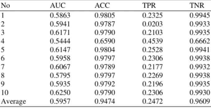
Table 1: Result for using SVM on the NCI data set
No AUC ACC TPR TNR
1 0.5863 0.9805 0.2325 0.9945
2 0.5941 0.9787 0.0203 0.9933
3 0.6171 0.9790 0.2103 0.9935
4 0.5444 0.6590 0.4539 0.6662
5 0.6147 0.9804 0.2528 0.9941
6 0.5958 0.9797 0.2306 0.9938
7 0.6067 0.9789 0.2177 0.9932
8 0.5795 0.9797 0.2269 0.9938
9 0.5935 0.9792 0.2196 0.9935
10 0.6250 0.9790 0.2306 0.9930
Average 0.5957 0.9474 0.2472 0.9609
Table 2: Result for using balanced SVM (balanced ridge = 0.01) on the NCI data set
No AUC ACC TPR TNR
1 0.5997 0.9793 0.2583 0.9928
2 0.6070 0.9781 0.2269 0.9922
3 0.6304 0.9784 0.2417 0.9922
4 0.5961 0.9794 0.2325 0.9934
5 0.6249 0.9793 0.2768 0.9925
6 0.6141 0.9792 0.2638 0.9926
7 0.6216 0.9783 0.2417 0.9921
8 0.5943 0.9791 0.2528 0.9927
9 0.6033 0.9780 0.2380 0.9919
10 0.6397 0.9786 0.2602 0.9922
Average 0.6131 0.9788 0.2491 0.9925
Table 3: Result for using bagging of balanced SVM (balanced ridge = 0.01) on the NCI data set
No AUC ACC TPR TNR
1 0.7326 0.6777 0.6495 0.6781
2 0.7433 0.6806 0.6753 0.6806
3 0.7491 0.6827 0.6679 0.6829
4 0.7372 0.6819 0.6568 0.6825
5 0.7449 0.6839 0.6845 0.6842
6 0.7446 0.6806 0.6697 0.6807
7 0.7477 0.6771 0.6864 0.6771
8 0.7535 0.6797 0.6845 0.6795
9 0.7551 0.6779 0.6900 0.6774
10 0.7449 0.6851 0.6827 0.6852
Average 0.7453 0.6807 0.6753 0.6808
has one third of the training data set, while for AB-SVM, the size of individual data subset is twice of the positive sample in the whole data set. The 3-fold cross validation scheme is used to validate the results, experiments on each algorithm are repeated 10 times.
DISCUSSION
Table 1-6 list the results of ordinary SVM, balanced-SVM, bagging of balanced-SVM, ordinary bagging, AB-SVM and SPRAG (special prediction risk based feature selection for asymmetric bagging), from which we can see that:
• Balanced SVM obtained a slight improvement of ordinary SVM
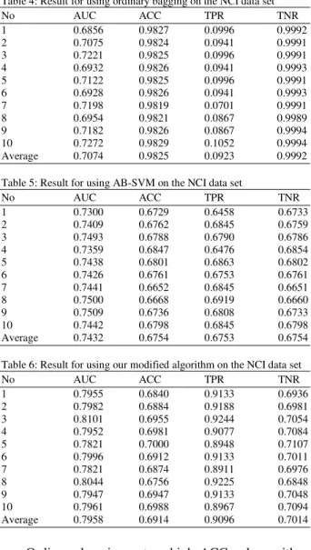
Table 4: Result for using ordinary bagging on the NCI data set
No AUC ACC TPR TNR
1 0.6856 0.9827 0.0996 0.9992
2 0.7075 0.9824 0.0941 0.9991
3 0.7221 0.9825 0.0996 0.9991
4 0.6932 0.9826 0.0941 0.9993
5 0.7122 0.9825 0.0996 0.9991
6 0.6928 0.9826 0.0941 0.9993
7 0.7198 0.9819 0.0701 0.9991
8 0.6954 0.9821 0.0867 0.9989
9 0.7182 0.9826 0.0867 0.9994
10 0.7272 0.9829 0.1052 0.9994
Average 0.7074 0.9825 0.0923 0.9992
Table 5: Result for using AB-SVM on the NCI data set
No AUC ACC TPR TNR
1 0.7300 0.6729 0.6458 0.6733
2 0.7409 0.6762 0.6845 0.6759
3 0.7493 0.6788 0.6790 0.6786
4 0.7359 0.6847 0.6476 0.6854
5 0.7438 0.6801 0.6863 0.6802
6 0.7426 0.6761 0.6753 0.6761
7 0.7441 0.6652 0.6845 0.6651
8 0.7500 0.6668 0.6919 0.6660
9 0.7509 0.6736 0.6808 0.6733
10 0.7442 0.6798 0.6845 0.6798
Average 0.7432 0.6754 0.6753 0.6754
Table 6: Result for using our modified algorithm on the NCI data set
No AUC ACC TPR TNR
1 0.7955 0.6840 0.9133 0.6936
2 0.7982 0.6884 0.9188 0.6981
3 0.8101 0.6955 0.9244 0.7054
4 0.7952 0.6981 0.9077 0.7084
5 0.7821 0.7000 0.8948 0.7107
6 0.7996 0.6912 0.9133 0.7011
7 0.7821 0.6874 0.8911 0.6976
8 0.8044 0.6756 0.9225 0.6848
9 0.7947 0.6947 0.9133 0.7048
10 0.7961 0.6988 0.8967 0.7094
Average 0.7958 0.6914 0.9096 0.7014
• Ordinary bagging gets a high ACC value, with a proper AUC value, but TPR is very low, which means that few of the positive examples are predicted correctly
• AB-SVM reduces the ACC value, but improves the AUC value of ordinary bagging. TPR increases from 9.23-67.53%
• PRIFEB improves both the ACC and AUC values of AB-SVM, TPR are improved dramatically and it is 90.96% in average
As for the above results, we think that:
• Since single SVM is not stable and can not obtain valuable results and bagging can improve them • Although ordinary bagging gets a high ACC value,
it is trivial, because few positive examples are
predicted correctly. If we simply predict all the labels as negative, we can get a high value as 98.15%, which is the ratio of negative sample to the whole sample
• Since this is a drug discovery problem, we pay more attention to positives. AUC is more valuable than ACC to measure a classifier. Asymmetric bagging improves the AUC value of ordinary bagging and our modified algorithm further significantly improves it to a higher one 79.58% in average, simultaneously, TPR are improved from 9.23-90.95%, which shows our modified algorithm is proper to solve the unbalanced drug discovery problem.
• Asymmetric bagging wins in two aspects, one is that it make the individual data subset balanced, the second is that it pay more attention to the positives and always put the positives in the data set, which makes TPR is higher than ordinary bagging and AUC is improved
• Feature selection using prediction risk as criterion also wins in two aspects, one is that embedded feature selection is dependent with the used learning machine, it will select features which benefit the generalization performance of individual classifiers, the second is that different features selected for different individual data subsets, which makes more diversity of bagging and improves their whole performance.
CONCLUSION
771
REFERENCES
1. Pugazhenthi, D. and S.P. Rajagopalan, 2007. Machine learning technique approaches in drug discovery, design and development. Inform.
Technol. J., 6: 718-724.
http://198.170.104.138/itj/2007/718-724.pdf 2. Tominaga, Y., 1999. Comparative study of class
data analysis with PCA-LDA, SIMCA, PLS, ANNs and k-NN. Chemometr. Intel. Lab. Syst., 49: 105-115. DOI: 10.1016/S0169-7439(99)00034-9
3. Tang, K. and T. Li, 2002. Combining PLS with GA-GP for QSAR. Chemometr. Intel. Lab. Syst., 64: 55-64. DOI: 10.1016/S0169-7439(02)00050-3 4. Fang, K.T., H. Yin and Y.Z. Liang, 2004. New
approach by kriging models to problems in QSAR. J. Chem. Inform. Comput. Sci., 44: 2106-2113. http://cat.inist.fr/?aModele=afficheN&cpsidt=1631 4722
5. Xue, Y., Z.R. Li, C.W. Yap, L.Z. Sun, X. Chen and Y.Z. Chen, 2004. Effect of molecular descriptor feature selection in support vector machine classification of pharmacokinetic and toxicological properties of chemical agents. J. Chem. Inform.
Comput. Sci., 44: 1630-1638.
http://www.ncbi.nlm.nih.gov/pubmed/15446820 6. Chen, N.Y., W.C. Lu, J. Yang and G.Z. Li, 2004.
Support Vector Machines in Chemistry. World Scientific Publishing Company, Singapore, ISBN: 10: 9812389229, pp: 331.
7. Bhavani, S., A. Nagargadde, A. Thawani, V. Sridhar and N. Chandra, 2006. Substructure based support vector machine classifiers for prediction of adverse effects in diverse classes of drugs. J. Chem.
Inform. Model., 46: 2478-2486.
http://eprints.iisc.ernet.in/9174/
8. Dietterich, T., 1998. Machine-learning research: Four current directions. AI Mag., 18: 97-136. http://direct.bl.uk/bld/PlaceOrder.do?UIN=040649 931&ETOC=RN&from=searchengine
9. Schapire, R.E., 1990. The strength of weak learnability. Mach. Learn., 5: 197-227. http://portal.acm.org/citation.cfm?id=83645 10. Breiman, L., 1996. Bagging predictors. Mach.
Learn., 24: 123-140.
http://portal.acm.org/citation.cfm?id=231989 11. Bauer, E. and R. Kohavi, 1999. An empirical
comparison of voting classification algorithms: Bagging, boosting and variants. Mach. Learn., 36: 105-139.
http://portal.acm.org/citation.cfm?id=599607
12. Agrafiotis, D.K., W. Cedeno and V.S. Lobanov, 2002. On the use of neural network ensembles in QSAR and QSPR. J. Chem. Inform. Comput. Sci., 42: 903-911.
http://www.ncbi.nlm.nih.gov/pubmed/12132892 13. Lanctot, J.K., S. Putta, C. Lemmen and J. Greene,
2003. Using ensembles to classify compounds for drug discovery. J. Chem. Inform. Comput. Sci., 43: 2163-2169.
http://www.ncbi.nlm.nih.gov/pubmed/14632468 14. Guha, R. and P.C. Jurs, 2004. Development of
linear, ensemble and nonlinear models for the prediction and interpretation of the biological activity of a set of PDGFR inhibitors. J. Chem. Inform. Comput. Sci., 44: 2179-2189. http://pubs.acs.org/doi/abs/10.1021/ci049849f 15. Dutta, D., R. Guha, D. Wild and T. Chen, 2007.
Ensemble feature selection: Consistent descriptor subsets for multiple QSAR models. J. Chem.
Inform. Model., 47: 989-997.
http://www.ncbi.nlm.nih.gov/pubmed/17407280 16. Eitrich, T., A. Kless, C. Druska, W. Meye and
J. Grotendorst, 2007. Classification of highly unbalanced CYP450 data of drugs using cost sensitive machine learning techniques. J. Chem.
Inform. Model., 47: 92-103.
http://cat.inist.fr/?aModele=afficheN&cpsidt=1857 0580
17. Tao, D., X. Tang, X. Li and X. Wu, 2006. Asymmetric bagging and random subspace for support vector machines based relevance feedback in image retrieval. IEEE Trans. Patt. Anal. Mach.
Intel., 28: 1088-1099. DOI:
10.1109/TPAMI.2006.134
18. Hand, D.J., 1997. Construction and Assessment of Classification Rules. Wiley, Chichester, ISBN: 10: 0471965839, pp: 232.
19. Li, G.Z., T.Y. Liu and V.S. Cheng, 2006. Classification of brain glioma by using SVMs bagging with feature selection. Lecture Notes Comput. Sci., 3916: 124-130. DOI: 10.1007/11691730_13
20. Yu, L. and H. Liu, 2004. Efficient feature selection via analysis of relevance and redundancy. J. Mach.
Learn. Res., 1205-1224.
http://portal.acm.org/citation.cfm?id=1044700 21. Kohavi, R. and G.H. John, 1997. Wrappers for
feature subset selection. Artif. Intel., 97: 273-324. http://portal.acm.org/citation.cfm?id=270627 22. Guyon, I. and A. Elisseeff, 2003. An introduction
to variable and feature selection. J. Mach. Learn.
Res., 3: 1157-1182.
23. Liu, Y., 2004. A comparative study on feature selection methods for drug discovery. J. Chem. Inform. Comput. Sci., 44: 1823-1828. http://pubs.acs.org/doi/abs/10.1021/ci049875d 24. Li, H., C.W. Yap, C.Y. Ung, Y. Xue, Z.W. Cao
and Y.Z. Chen, 2005. Effect of selection of molecular descriptors on the prediction of blood-brain barrier penetrating and nonpenetrating agents by statistical learning methods. J. Chem. Inform. Model., 45: 1376-1384.
http://pubs.acs.org/doi/abs/10.1021/ci050135u 25. Li, G.Z., J. Yang, G.P. Liu and L. Xue, 2004.
Feature selection for multi-class problems using support vector machines. Lecture Notes Comput. Sci., 3157: 292-300. DOI: 10.1007/b99563
26. Boser, B.E., I.M. Guyon and V.N. Vapnik, 1992. A training algorithm for optimal margin classifiers. Proceedings of the 5th Annual Workshop on Computational Learning Theory, July 27-29, ACM Press, Pittsburgh, Pennsylvania, United
States, pp: 144-152.
http://portal.acm.org/citation.cfm?id=130401 27. Cristianini N. and J. Shawe-Taylor, 2000. An
Introduction to Support Vector Machines: And other Kernel-Based Learning Methods.Cambridge University Press, Cambridge, ISBN: 0521780195, pp: 189.
28. Guyon, I., J. Weston, S. Barnhill and V. Vapnik, 2002. Gene selection for cancer classification using support vector machines. Mach. Learn., 46: 389-422. http://portal.acm.org/citation.cfm?id=599671 29. Vapnik, V.N., 1998. Statistical Learning Theory.
Wiley, New York,ISBN: 10: 0471030031, pp: 736. 30. Karush, W., 1939. Minima of functions of several
variables with inequalities as side constraints. Master's Thesis, Department of Mathematics, University of Chicago, Chicago. http://www.bibsonomy.org/bibtex/282efea517f19c 5edff001dd4b359b70b/sb3000
31. Kuhn, H.W. and A.W. Tucker, 1951. Nonlinear programming. Proceeding of the 2nd Berkeley Symposium on Mathematical Statistics and Probability, July 31-Aug. 12, University of California Press, Berkeley and Los Angles, California, pp: 1-9.
32. Mercer, J., 1909. Functions of positive and negative type and their connection with the theory of integral equations. Philosophic. Trans. R. Soc.
Lond., 209: 415-446.
http://adsabs.harvard.edu/abs/1909RSPTA.209..415M 33. Hsu, C.W., C.C. Chang and C.J. Lin, 2003. A
practical guide to support vector classification. Tech rep 2003 Department of Computer Science
and Information Engineering, National Taiwan University, Taiwan.
http://www.csie.ntu.edu.tw/~cjlin/papers/guide/gui de.pdf
34. Chang, C.C. and C.J. Lin, 2007. LIBSVM-A library for support vector machines version 2.85 http://www.csie.ntu.edu.tw/~cjlin/libsvm/index.ht ml
35. Li, G.Z. and T.Y. Liu, 2006. Feature selection for bagging of support vector machines. Lecture Notes Comput. Sci., 4099: 271-277. DOI: 10.1007/978-3-540-36668-3
36. Moody, J. and J. Utans, 1992. Principled Architecture Selection for Neural Networks: Application to Corporate Bond Rating Prediction. In: Advances in Neural Information Processing Systems, Moody, J.E., S.J. Hanson and R.P. Lippmann (Eds.). Morgan Kaufmann Publishers, Inc., pp: 683-690. http://www.icsi.berkeley.edu/cgi-bin/pubs/publication.pl?ID=001490
37. Duda, R.O., P.E. Hart and D.G. Stork, 2000. Pattern Classification. 2nd Edn., Wiley- Interscience,ISBN: 10: 0471056693, pp: 654. 38. Todeschini, R., V. Consonni, R. Mannhold, H. Kubinyi
and H. Timmerman,2000. Handbook of Molecular Descriptors. 1st Edn., Wiley-VCH., Germany, ISBN: 10: 3527299130, pp: 688.
39. Young, S.S., V.K. Gombar, M.R. Emptage, N.F. Cariello and C. Lambert, 2002. Mixture deconvolution and analysis of ames mutagenicity data. Chemomet. Intel. Lab. Syst., 60: 5-11. DOI: 10.1016/S0169-7439(01)00181-2
40. Feng, J., L. Lurati, H. Ouyang, T. Robinson, Y. Wang, S. Yuan and S.S. Young, 2003. Predictive toxicology: Benchmarking molecular descriptors and statistical methods. J. Chem. Inform. Comput.
Sci., 43: 1463-1470.
http://cat.inist.fr/?aModele=afficheN&cpsidt=1518 1463