http://dx.doi.org/10.1590/2318-0331.011615094
RBRH, Porto Alegre, v. 21, n. 3, p. 646-651, jul./set. 2016 Technical Note
Cumulative equations for continuous time Chicago hyetograph method
Equações cumulativas sequenciais do hietograma do método de Chicago
André Luiz Lopes da Silveira1
1Universidade Federal do Rio Grande do Sul, Porto Alegre, RS, Brazil
E-mail: [email protected] (ALLS)
Received: June 17, 2015 - Revised: March 28, 2016 - Accepted: April 05, 2016
ABSTRACT
The Chicago method is a classical method based on IDF curves for obtaining design hyetographs which present rainfall rates as continuous functions of time, one valid for times before peak and another for after peak. The intensity peak of rainfall is arbitrarily positioned at time zero, the function before peak counting time reversely and the function after peak with time axis normally. The time duration of the hyetograph before peak is determined by multiplying the total duration by a displacement factor with value between zero and one. This technical note presents both equations for before and after peak with the same time axis (time zero at the beginning of hyetograph) to facilitate applications of the Chicago method. The equations presented show cumulated rainfall depths resulting from exact integrals over chronological time of the original Chicago method’s rainfall intensity equations. That is, at every instant of time from the beginning of the hyetograph one has the exact value of cumulated rainfall. Thus, by decumulation, the sequential rainfall hyetograph depths are obtained. There is an advantage in using these equations which are easily introduced in spreadsheets.
Keywords: Chicago method; Design hyetograph; IDF.
RESUMO
O método de Chicago é um dos métodos clássicos em hidrologia para deinição de hietogramas de projeto com base nas curvas de intensidade-duração-frequência (curvas IDF). O hietograma do método de Chicago apresenta as intensidades por funções contínuas no tempo, uma para antes e outra para depois do pico. O pico é posicionado arbitrariamente em um instante zero e as equações usam tempos contados de forma reversa (antes do pico) ou normal (depois do pico). A duração para antes do pico é determinada por um fator de pico entre zero e um multiplicado pela duração total do hietograma. Para facilitar o emprego do método de Chicago a presente nota técnica apresenta equações com tempo zero na origem do hietograma e valores obtidos de forma cronológica até a sua duração total. As equações aqui apresentadas são de precipitações cumulativas que representam a integral exata no tempo dos volumes das intensidades do Método de Chicago, ou seja, a cada instante de tempo a partir de zero (início da chuva) tem-se o valor exato da lâmina acumulada precipitada. Por desacumulação podem-se obter as lâminas precipitadas sequenciais do hietograma. Há uma vantagem de manuseio dessas equações que as tornam facilmente programáveis em planilhas eletrônicas.
INTRODUCTION
The well-known “Chicago Method” was proposed by Keifer and Chu (1957) to calculate design rainfalls of urban storm water infrastructures. The method establishes two analytical equations for rainfall intensity over time, one valid before the peak rate and another valid after peak, both deduced from an IDF (intensity-duration-frequency) analytical expression, preserving the same volumes of all rainfall intensities.
The Chicago method is much utilized worldwide, but
it should be emphasized that it calculates an artiicial rainfall
hyetograph as a design hyetograph, which the time distribution derives from the analytical expression of IDF without any relationship with real hyetographs patterns. Even if this method considers a parameter to locate the peak rate in time, estimated from real hyetographs, this conclusion does not change. Despite this, Alfieri, Laio and Claps (2008), after testing ive design hyetographs by simulation, concluded that the Chicago method
results are consistent and stable in low calculations with several
unit graphs applied to different watershed and climate parameters.
They noted a systematic overestimation of lows, which could be
corrected by a factor of 0.94.
This technical note does not aim to discuss different approaches to calculate design hyetographs. The focus is on the classical Chicago method, so the objective of this paper is to present the chronological and continuous cumulative equations of rainfall depths, to facilitate the calculation of design hyetographs by simple handheld calculators or electronic spreadsheets without requiring the use of complex software packages. The equations presented here do not need any integration because they provide cumulative rainfall depths directly, in a form not normally described in hydrology text books. While a software manual (SMITH, 2004) contains cumulative rainfall depth equations, as opposed to those that are presented in this technical note, they do not calculate chronological cumulative rainfall depths from the beginning to the end of rainfall duration.
CHICAGO METHOD
The method starts with an analytical and time differentiable IDF equation. Therefore, it is possible to employ the Sherman equation (GARCIA-BARTUAL; SCHNEIDER, 2001) presented below:
( )
t n
a i
t b
=
+ (1)
Where it is the rainfall intensity, t is the duration, a, b and n being the parameters that represent local conditions and the return period, the latter considered in the parameter “a” by an expression such as this:
m
a=k T (2)
Where T is the return period in years and k a constant.
When n=1 and b > 0 the IDF equation is normally called the Talbot equation. When b=0 and n > 0 the equation is known as Montana equation.
The Chicago method development starts from the volume equation associated with the intensity of IDF for each t, that is, the product of IDF intensity by its duration t, resulting in:
( )
t n
a t V
t b
=
+ (3)
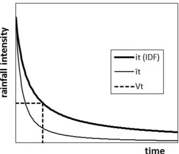
The method considers an average rainfall intensity function
curve īt, different from it, which integral over time match the
volume Equation 3 above:
( )
t
t t
0 n
a t i dt V
t b
= = +
∫ (4)
Doing a derivation dVt/dt, results in:
( ) ( )
t 1 n
a t 1 n b
i
t b +
− +
=
+ (5)
This equation has a maximum intensity for t = 0, as for
the IDF equation. However, except for t=0, where the intensities
are equal, it is clear that:
t t
i <i (6)
Figure 1 shows these intensity functions, where a rectangle area indicates the volume Vt.
The innovative idea by Keifer and Chu (1957) was to use
a modiied Equation 5 to explain hyetograph intensities after
the peak, and a similar one, reversed, for intensities before peak.
In other words the peak is ixed at t = 0, a modiied Equation 5
on a normal t axis is then used for after peak intensities. Another
modiied Equation 5 with an opposed t axis provides before peak
intensities. Thus, to maintain the same volume of Equation 5
both modiied equations, representing a unique hyetograph, incorporate a peak factor γ, ranging from 0 to 1, known as storm advancement coeficient. In fact, the γ parameter locates the
hyetograph peak intensity over its duration. Before the peak the
modiied Equation 5 replaces the t variable of the opposite axis
by t1/γ. After the peak the modiied Equation 5 replaces the t variable of a normal axis by t2/(1-γ).
As a result of this the well-known rainfall intensity equations of the Chicago method are obtained, given by:
Before peak
( )
1
1
t 1 n
1
t
a 1 n b
i t
b
+
− +
=
+
γ
γ
(7)
After peak
( )
2
2
t 1 n
2
t
a 1 n b
1 i
t b 1
+
− +
−
=
+ −
γ
γ
(8)
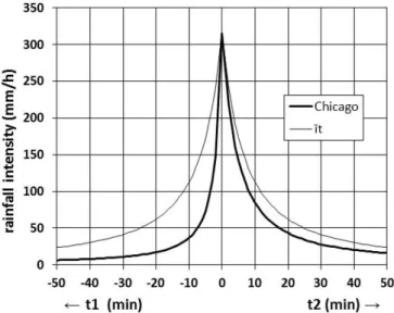
Figure 2 shows both opposite axes (t1 and t2) each of them
with their ī function. The example considered the Porto Alegre (Brazil) IDF at INMET (National Meteorology Institute) station
(BEMFICA; GOLDENFUM; SILVEIRA, 2000), with a return
period of T = 50 years and γ = 0.3.
CUMULATIVE EQUATIONS
The contribution of this technical note is a sequential integration of Equations 7 and 8 over an interval (0,t), where
t = 0 identiies the beginning of whole hyetograph. As a result
two cumulative rainfall equations (providing rainfall cumulative depths from the beginning of the hyetograph) are obtained.
The irst is valid for times before tp, the time peak. The second
is valid for times after the peak. Before peak
(
p)
t TOT n
p
a t t
P P
t t
b
−
= −
−
+
γ
γ
(9)
After peak
(
p)
t TOT n
p
a t t
P P
t t b
1
−
= +
−
+ −
γ
γ
(10)
Where Pt is the cumulative rainfall at time t from the beginning of the hyetograph.
PTOT, the total rainfall depth of the hyetograph is given by:
( TOT)
TOT n
TOT
a t P
t b
=
+ (11)
Where tTOT is the total duration of the hyetograph.
It should be mentioned that Equations 9 and 10 are exact integrals over time of intensities given by the Chicago method,
that is, Equations 9 and 10 do not introduce any simpliication
and are valid for an IDF like Equation 1.
Example 1
The example 5.10 of Bertoni and Tucci (1993) was irst taken to demonstrate the performance of Equations 9 and 10.
Without specifying location these authors utilized the following IDF equation:
( ) . .
0 15
t 0 75
1100 T i
t 30
=
+ (12)
Where it is the rainfall intensity in mm/h, T is the return period in years and t the time in minutes.
The example of Bertoni and Tucci (1993) presents an application of the Chicago method for a hyetograph with total duration of 90 minutes, time step of 10 minutes, return period
of 10 years and γ = 0.35.
The irst step is to calculate the parameter “a”. This
parameter is simply the IDF numerator divided by 60 to obtain intensities in mm/min, consistent with time t in minutes.
.
.
0 15
1100 10
a 25 90
60
×
= = (13)
Parameters “b” and “c” were taken directly from IDF:
min
b=30 (14)
.
c=0 75 (15)
With tTOT = 90 min, Equation 11 provides:
( ).
.
.
TOT 0 75
25 90 90
P 64 29 mm
90 30
×
= =
+ (16)
Figure 2. Mirrored īt functions and those of the Chicago hyetograph
Thus,
. . .
TOT
P =0 35 64 29× =22 50 mm
γ (17)
The peak time is given by:
. . min
p TOT
t =γt =0 35 90× =31 5 (18)
With these parameter values the resulting cumulative rainfall equations are:
Before peak (t <= 31.5 min)
( ) . . . . . .
t 0 75
25 90 31 5 t P 22 50
31 5 t 30 0 35 − = − − + (19)
After peak (t>= 31.5 min)
( ) . . . . . .
t 0 75
25 90 t 31 5 P 22 50
t 31 5 30 0 65 − = + − + (20)
The results of Equations 19 and 20 are presented in Table 1 (Pt), with the corresponding non cumulated values which are the hyetograph rainfall depths. The last column of Table 1 shows the hyetograph values by Bertoni and Tucci (1993).
Except for rounding errors, the results of Equations 19 and 20 are virtually the same shown in Bertoni and Tucci (1993) denoting the correction of the proposed Equations 9 and 10.
Example 2
A second example for the evaluation of Equations 9 and 10 is given by Zahed Filho and Marcellini (1995) example 2.4.
The IDF equation utilized by these authors was provided
by Paulo Sampaio Wilken for São Paulo (Brazil):
( ) . .
. 0 172
t 1 025
3462 7 T i
t 22
=
+ (21)
Where it is the rainfall intensity in mm/h, T is the return period in years and t the time in minutes.
The example of Zahed Filho and Marcellini (1995) presents an application of the Chicago method for a hyetograph with a total duration of 90 minutes, time step of 5 minutes, return period
of 10 years and γ = 0.39.
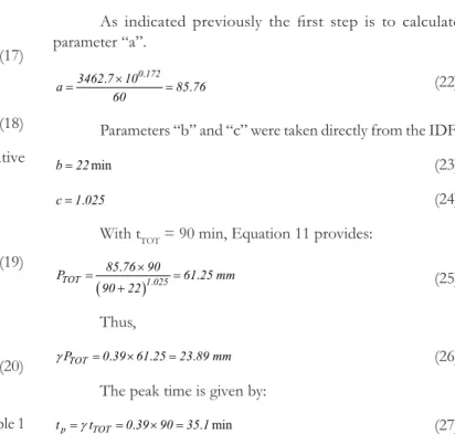
As indicated previously the irst step is to calculate
parameter “a”.
.
.
.
0 172
3462 7 10
a 85 76
60
×
= = (22)
Parameters “b” and “c” were taken directly from the IDF:
min
b=22 (23)
.
c=1 025 (24)
With tTOT = 90 min, Equation 11 provides:
( ).
.
.
TOT 1 025
85 76 90
P 61 25 mm
90 22
×
= =
+ (25)
Thus,
. . .
TOT
P =0 39 61 25× =23 89 mm
γ (26)
The peak time is given by:
. . min
p TOT
t =γt =0 39 90× =35 1 (27)
With these parameter values the resulting cumulative rainfall equations are:
Before peak (t <= 35.1 min)
( ) . . . . . .
t 1 025
85 76 35 1 t P 23 89
35 1 t 22 0 39 − = − − + (28)
After peak (t>= 35.1 min)
( ) . . . . . .
t 1 025
85 76 t 35 1 P 23 89
t 35 1 22 0 61 − = + − + (29)
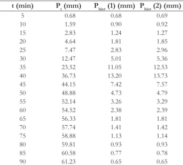
Equations 28 and 29 were applied with a 5 min step providing cumulated values Pt (Table 2). The corresponding non cumulated values which are the hyetograph rainfall depths were shown in the second column. The last column of Table 2 shows the hyetograph values by Zahed Filho and Marcellini (1995).
It can be observed that results of the proposed Equations 9 and 10 are very similar to those obtained by Zahed Filho and Marcellini (1995). The differences noted are due to the fact that these authors calculated rainfall depths by averaging rainfall intensities of the beginning and end of each time step, while this technical note equation provides exact integrals over the entire time interval curve. The total rainfall calculated by Zahed Filho and Marcellini (1995) has rounding errors because the sum of last column values is 64 mm, slightly different from the expected value (61.2 mm) of IDF with a total duration of 90 minutes.
Example 3
Example 3 is provided by AAS (SMITH, 2004), in which
IDF, with a ixed 5 year return period, does not have a speciied
location: Table 1. Results of Example 1.
t (min) Pt (mm) Phiet (1) (mm) Phiet (2) (mm)
10 3.67 3.67 3.66
20 9.16 5.49 5.49
30 19.76 10.60 10.60
40 35.59 15.83 15.83
50 45.16 9.57 9.54
60 51.80 6.64 6.67
70 56.85 5.05 5.04
80 60.90 4.05 4.06
90 64.29 3.39 3.38
( ).
t 0 84
1140 i
t 6
=
+ (30)
Where it is the rainfall intensity in mm/h and t is the time in minutes. The AAS (SMITH, 2004) hyetograph example has a total duration of 120 minutes with 5 minute time intervals. The peak
factor was γ = 0.35. The return period (5 years) was ixed in the IDF.
As shown before, parameter “a” is the numerator of the IDF equation divided by 60.
.
1140
a 19 00
60
= = (31)
Parameters “b” and “c” are issued directly from IDF:
min
b=6 (32)
.
c=0 84 (33)
tTOT = 120 min being the total duration of the hyetograph, Equation 11 provides:
( ).
.
.
TOT 0 84
19 00 120
P 39 23 mm
120 6
×
= =
+ (34)
Thus,
. . .
TOT
P =0 35 39 23× =13 73 mm
γ (35)
The peak time is given by:
. . min
p TOT
t =γt =0 35 120× =42 0 (36)
Replacing the above parameter values in Equations 9 and 10, results for this case in the cumulative equations for rainfall:
Before peak (t <= 42.0 min)
( )
.
. .
.
. .
t 0 84
19 00 42 0 t P 13 73
42 0 t 6
0 35
−
= −
−
+
(37)
After peak (t>= 42.0 min)
( )
.
. .
.
. .
t 0 84
19 00 t 42 0 P 13 73
t 42 0 6
0 65
−
= +
−
+
(38)
Equations 37 and 38 when applied in 5 minute steps give the cumulative values of Table 3 with their corresponding non cumulated ones (the hyetograph). The results from AAS (SMITH, 2004) are also presented for comparison.
It can be seen in Table 3 that the hyetograph obtained by cumulative equations is identical to those of AAS (SMITH, 2004).
CONCLUSION
Cumulative rainfall equations of the Chicago hyetograph method are presented considering time from zero (beginning of
hyetograph) to total duration (ending of hyetograph). Normally,
this does not happen, because classical Chicago equations consider peak at time zero and regressive time counting for intensities before peak and progressive counting for after peak. This technical note thus presents a unique timeline from beginning to end of the hyetograph for rainfall calculation. An equation “before peak” gives the cumulated rainfall from beginning to time peak hyetograph. A second one, an “after peak” equation, is applied for times after time peak to ending and gives the cumulated rainfall from the beginning of the hyetograph. The absolute rainfall blocks are then obtained by subtracting the cumulated values between two time steps.
Table 2. Results of Example 2.
t (min) Pt (mm) Phiet (1) (mm) Phiet (2) (mm)
5 0.68 0.68 0.69
10 1.59 0.90 0.92
15 2.83 1.24 1.27
20 4.64 1.81 1.85
25 7.47 2.83 2.96
30 12.47 5.01 5.36
35 23.52 11.05 12.53
40 36.73 13.20 13.73
45 44.15 7.42 7.57
50 48.88 4.73 4.79
55 52.14 3.26 3.29
60 54.52 2.38 2.39
65 56.33 1.81 1.81
70 57.74 1.41 1.42
75 58.88 1.13 1.14
80 59.81 0.93 0.93
85 60.58 0.77 0.78
90 61.23 0.65 0.65
(1) Results of this technical note calculated by an electronic spreadsheet; (2) Results of Zahed Filho and Marcellini (1995).
Table 3. Results of Example 3.
t (min) Pt (mm) Phiet (1) (mm) Phiet (2) (mm)
5 0.35 0.35 0.35
10 0.75 0.40 0.40
15 1.21 0.47 0.47
20 1.78 0.57 0.57
25 2.51 0.72 0.72
30 3.51 1.00 1.00
35 5.11 1.61 1.61
40 8.92 3.81 3.81
45 21.57 12.65 12.65
50 39.23 5.38 5.38
55 26.95 2.78 2.78
60 29.73 1.82 1.82
65 31.55 1.34 1.34
70 32.89 1.05 1.05
75 33.94 0.87 0.87
80 34.81 0.74 0.74
85 35.54 0.64 0.64
90 36.18 0.57 0.57
95 36.75 0.51 0.51
100 37.26 0.46 0.46
105 37.72 0.42 0.42
110 38.14 0.39 0.39
115 38.53 0.36 0.36
120 38.89 0.34 0.34
The equations provided by this technical note are advantageous for use in simple electronic spreadsheets, besides the fact they are exact integrals of original intensity curves by Keifer and Chu (1957). Three different examples are presented to demonstrate the proposed cumulative equations. The method is valid for any IDF with mathematical expression of Sherman, Talbot or Montana (GARCIA-BARTUAL; SCHNEIDER, 2001).
This technical note is not aimed at also validating the Chicago method. For novice users it must be highlighted that the Chicago method was originally developed to calculate stormwater hyetographs with any duration for design of urban drainage infrastructures but not limited to these conditions (BERTONI; TUCCI, 1993). The Chicago method considers the same return period for the entire hyetograph, and this can cause overestimation. Alfieri, Laio and Claps (2008) demonstrated this overestimation, by experiments with the simulation of convolution of Chicago hyetographs by general unitgraphs, and concluded that overestimations are small and can be corrected by using a multiplying factor of 0.94.
REFERENCES
ALFIERI, L.; LAIO, F.; CLAPS, P. Simulation experiment for optimal design hyetograph selection. Hydrological Processes, v. 22, n. 6, p. 813-820, 2008. http://dx.doi.org/10.1002/hyp.6646.
BEMFICA, D. C.; GOLDENFUM, J. A.; SILVEIRA, A. L. L.
Análise da aplicabilidade de padrões de chuva de projeto a Porto
Alegre. Revista Brasileira de Recursos Hídricos, v. 5, n. 4, p. 5-16, 2000. http://dx.doi.org/10.21168/rbrh.v5n4.p5-16.
BERTONI, J. C.; TUCCI, C. E. M. Precipitação. In: TUCCI, C. E. M. Hidrologia: ciência e aplicação. Porto Alegre: Editora da Universidade, 1993. cap. 5, p. 177-241.
GARCIA-BARTUAL, R.; SCHNEIDER, M. Estimating maximum expected short-duration rainfall intensities from extreme convective storms. Physics and Chemistry of the Earth, Part B: Hydrology, Oceans and Atmosphere, v. 26, n. 9, p. 675-681, 2001. http://dx.doi. org/10.1016/S1464-1909(01)00068-5.
KEIFER, C. J.; CHU, H. H. Synthetic storm pattern for drainage design. Journal of the Hydraulics Division, v. 83, p. 1-25, 1957.
SMITH, A. A. MIDUSS Version 2: reference manual. Ontario: AAS, 2004. Available from; <http: www.midussware.com/files/ MIDUSSv2Tutorial.pdf>. Access on: 15 mar. 2016.