www.ache.org.rs/CICEQ
Chemical Industry & Chemical Engineering Quarterly 19 (3) 321−331 (2013) CI&CEQ
HASSAN GOLMOHAMMADI1
ABBAS RASHIDI2
SEYED JABER SAFDARI1
1Nuclear Science and Technology
Research Institute, AEOI, Tehran, Iran
2
Department of Chemical Engineering, Faculty of Engineering, University of Mazandaran, Babolsar, Iran
SCIENTIFIC PAPER
UDC 66:004.8 DOI 10.2298/CICEQ120403066G
PREDICTION OF FERRIC IRON
PRECIPITATION IN BIOLEACHING PROCESS
USING PARTIAL LEAST SQUARES AND
ARTIFICIAL NEURAL NETWORK
A quantitative structure-property relationship (QSPR) study based on partial least squares (PLS) and artificial neural network (ANN) was developed for the prediction of ferric iron precipitation in bioleaching process. The leaching tem-perature, initial pH, oxidation/reduction potential (ORP), ferrous concentration and particle size of ore were used as inputs to the network. The output of the model was ferric iron precipitation. The optimal condition of the neural network was obtained by adjusting various parameters by trial-and-error. After optimi-zation and training of the network according to back-propagation algorithm, a 5-5-1 neural network was generated for prediction of ferric iron precipitation. The root mean square error for the neural network calculated ferric iron preci-pitation for training, prediction and validation set were 32.860, 40.739 and 35.890, respectively, which were smaller than those obtained by the PLS model (180.972, 165.047 and 149.950, respectively). The obtained results reveal the reliability and good predictivity of the neural network model for the prediction of ferric iron precipitation in bioleaching process.
Keywords: quantitative structure-property relationship; ferric iron preci-pitation; bioleaching process; partial least squares; artificial neural net-work.
Bioleaching employs the oxidation ability of bacteria to dissolve metal sulphides and help the extraction and recovery of valuable and base metals from main ores and concentrates [1,2]. Metal-winning processes derived from the activity of microorganisms propose a possibility to attain metal ions from mineral resources not available by traditional techniques. Mic-robes such as bacteria and fungi change metal com-pounds into their water-soluble types and are bioca-talysts of this process called microbial leaching or bioleaching [3,4]. Recently, Acidithiobacillus ferrooxi-dans were believed to be the common significant mic-roorganisms in the bioleaching of metal ions from ores [5].
Acidithiobacillus ferrooxidans is an acidophilic chemolithoautotrophic proteobacterium that achieves
Correspondence: H. Golmohammadi, Nuclear Science and Technology Research Institute, AEOI, P.O. Box 11365-3486, Tehran, Iran.
E-mail: [email protected] Paper received: 3 April, 2012 Paper revised: 20 June, 2012 Paper accepted: 20 June, 2012
its energy from the oxidation of ferrous iron, elemental sulfur, or partially oxidized sulfur compounds [6]. Owing to its capacity of oxidation, Acidithiobacillus ferrooxidans has abundant industrial appliances in biohydrometallurgy. The most important applications can be established in the field of mining [7] where the oxidative effects are utilized for the bioleaching of dif-ferent metals such as copper from minerals like pyrite or chalcopyrite [8,9] or even uranium [10].
The mechanism of uranium extraction assisted by the indirect oxidation purpose of this microbe is probably as follows:
UO2 + Fe2(SO4)3 → UO2SO4 + 2FeSO4 (1)
U4+ + 2Fe3+ → U6+ + 2Fe2+ (2)
Temperature and pH of leaching solution can vary widely in the completeness of time. In addition, as the values of this parameter increase, ferric iron precipitation increases and consequently the leaching efficiency reduce. Therefore, it is very important to predict ferric iron concentration recycled by a com-prehensive model for the design, monitoring and organization of bioleaching operations.
As an alternative to physical models, artificial neural networks (ANNs) are a valuable estimate tool. Up to now, numerous applications of ANN models in the engineering area were reported. For example, Laberge et al. applied ANN to predict the metal (Cu, Zn and Cd) solubilization percentages in municipal sludge treated with a continuous bioleaching process [11]. Jorjani et al. used ANN to estimate the effects of operational parameters on the organic and inorganic sulfur removal from coal by sodium butoxide [12]. Acharya and co-workers developed a neural network to model the extent of sulphur removal from three types of coal using native cultures of Acidithiobacillus ferrooxidans [13]. Diamond et al. utilized ANN for the Study of pH on the fungal treatment of red mud [14]. Nikhil et al. employed ANN for prediction of H2
pro-duction rates in a sucrose-based bioreactor system [15]. They also modeled the performance of a biolo-gical Fe2+ oxidizing fluidized bed reactor (FBR) by a
popular neural network-back-propagation algorithm under different operational conditions [16]. Yetilmez-soy and Demirel used a three-layer artificial neural network (ANN) model to predict the efficiency of Pb(II) ions removal from aqueous solution by Antep pista-chio (Pistacia vera L.) shells based on 66 experi-mental sets obtained in a laboratory batch study [17]. Daneshvar et al. employed an artificial neural network (ANN) to model decolorization of textile dye solution containing C.I. Basic Yellow 28 by electrocoagulation process [18]. Sahinkaya and co-workers developed an artificial neural network model for estimation of the performance of a fluidized-bed reactor (FBR) based sulfate reducing bioprocess and control the opera-tional conditions for improved process performance [19]. Sahinkaya also modeled the biotreatment of zinc-containing wastewater in a sulfidogenic CSTR by using artificial neural network [20].
Thus, to successfully extract the costly metals from the minerals, the suitable process and control of bioleaching purposes have become very essential. In relation to recent considerations, the dissolution of metals happens only chemically with the assist of fer-ric ions, which operate as oxidizing agents. Superior control of bioleaching may be acquired by using a strong model to predict convinced key factors derived
from past surveillances [21]. Models rooted in ANNs may be efficiently employed in bioleaching applica-tions and very helpful at arresting the nonlinear corre-lations existing between variables in complex systems like bioleaching. The main aim of this investigation is using this aptitude of artificial neural network for pre-diction of ferric iron precipitation in bioleaching pro-cess. In this study, an artificial neural network method using the back-propagation algorithm was proposed for the prediction of ferric iron precipitation in uranium bioleaching process under different operational conditions.
MATERIAL AND METHODS
Uranium ores
The uranium ores used in the experiments was supplied by the Nuclear Science and Technology Research Institute, AEOI. The ore was ground using mortar and then sieved. The particle size of the sieved material ranged from 70 to 500 µm, with an average particle size of 100±10 µm.
Microorganism and culture
The medium for Acidithiobacillus ferrooxidans growthwas 9K medium which is a mixture of mineral salts ((NH4)2SO4, 3.0 g/l, K2HPO4, 0.5 g/l, MgSO4⋅7H2O,
0.5 g/l, KCl, 0.1 g/l and Ca(NO3)2, 0.01g/l). FeSO4⋅7H2O
was added as energy source. The pH of the medium was adjusted to 2.0 using 2.0 M H2SO4. The culture
was cultivated at 35 °C for 2-3 days before centri-fugation. The yield cells of Acidithiobacillus ferrooxi-dans were suspended in a fresh solution of the mine-ral salt medium for the preparation of the bacterial concentrate [22].
Bioleaching experiments
The experiments were performed in 250 ml Erlenmeyer flasks containing 5 g of ore and 100 ml of 9K medium. Erlenmeyer flasks covered with hydro-phobic cotton to admit oxygen but reduce water loss through evaporation. Control experiments were car-ried out without bacteria and with 2% bactericide agent (formaldehyde). The concentrations of Fe were 2 and 4 g/l using FeSO4⋅7H2O. Each experiment was
Analytical procedures
Total iron was analyzed using the PG T80+ UV/Vis spectrometer according to Karamanev method [24]. The ferrous iron concentration was determined using PG T80+ UV/Vis spectrometer by the modified colorimetric orthophenantroline method [25]. A Metr-ohm pH meter (model 827) with a combined glass electrode was used for pH measurements. The changes in oxidation/reduction potential (ORP) were monitored using an ORP meter (Metrohm model 827). Partial least squares model for the prediction of ferric iron precipitation
PLS is a familiar multivariate method [26-28], which provides a stepwise solution for a regression model. It extracts principal component-like latent vari-ables from original independent varivari-ables (predictor variables) and dependent variables (response vari-ables), respectively. Assume that X characterizes independent variables (X is a matrix) and Y repre-sents dependent variables (Y is a vector). Then a brief description of computations is given as follows:
X = TPT + E (3)
Y = QST
+ F (4) The matrices E and F include residual for X and Y,
respectively. T and P are score and loading matrices associated with the X, Q and S are the score and loading of Y and superscript T indicates the trans-posed matrix. The relationship between scores and dependent variable is obtained from:
Y = TBQT
+ F (5) where B is the matrix of the regression coefficient
achieved by a least squares procedure. The PLS algorithm used in this study was the singular value decomposition (SVD)-based PLS. This algorithm was proposed by Lobert et al. in 1987 [29]. A concise discussion of the SVD-based PLS algorithm can be found in the literature [30-32]. The program of PLS modeling based on SVD was written with MATLAB 7 in our laboratory [33].
Artificial neural network model for the prediction of ferric iron precipitation
An artificial neural network is a kind of artificial intelligence that emulates some purpose of the human brain. Neural networks are general-purpose computing techniques that can solve complex non-linear problems. The network comprises abundance of simple processing elements linked to each other by weighted connections along with a specified architect-ure. These networks learn from the training data by
altering the connection weights [34]. A detailed expla-nation of the theory behind a neural network has been sufficiently described elsewhere [35-37]. Therefore, only the points related to this work are illustrated here. An essential procession element of an ANN is a node. Each node has a series of weighted inputs, Wij,
and performs as a summing point of weighted input signals. The summed signals pass through a transfer function that may be in sigmoidal form. The output of node j, Oj , is given by Eq.(6):
Oj = 1/(1 + exp(-X)) (6)
where X is defined by the following equation:
= W Oij i +Bj
X (7)
In Eq. (7), Bj is a bias term, Oi is the output of the
node of the previous layer and Wji represents the
weight between the nodes of i and j.
A feed-forward neural network consists of three layers. The first layer (input layer) consists of nodes and operates as an input buffer for the data. Signals introduced to the network, with one node per element in the sample data vector, pass through the input layer to the layer called the hidden layer. Each node in this layer sums the inputs and forwards them through a transfer function to the output layer. These signals are weighted and then pass to the output layer. In the output layer the processes of summing and transferring are repeated. The output of this layer now signifies the calculated value for the node k of the network.
As well as the network topology, a significant constituent of nearly all neural networks is a learning rule. A learning rule permits the network to alter its connection weights so as to correlate given inputs with corresponding outputs. The training of the net-work has been performed by using a back-propaga-tion algorithm, in which the network reads inputs and outputs from an appropriate data set (training set) and iteratively calculates weights and biases to facilitate decrease the sum of squared dissimilarities between predicted and target values. The training is stopped when the error in prediction achieves a preferred level of accuracy. However, if the network is gone to train too long, it will overtrain and misplace the aptitude to prediction. In order to avoid overtraining, the predict-ive recital of the trained ANN is controlled by running the back-propagation algorithm on a data set not used in training.
perfor-mance and properties of such a network is reliant on the computational elements, especially the weights and the transfer function, in addition to the net topo-logy. Usually the network topology and the transfer function are particular in advance and are kept fixed, so just the weights of the synaptic connections and the number of neurons in the hidden layer need to be evaluated. The error function should be minimized so that the neural network accomplishes the finest per-formance. Dissimilar algorithms have been grown to minimize the error function. The most traditional is the so-called back-propagation (BP) algorithm, which belongs to the group of supervised learning methods. The error at the output layer in a BP neural network propagates rearward to the input layer during the hid-den layer in the network to acquire the final beloved output. The gradient descent technique is employed to compute the weights of the network and regulate the weights of interconnections to minimize the output error. In this work, multi layered feed forward neural networks were used, which utilized the algorithm of back-propagation of errors and a gradient-descent technique, known as the “delta rule” [38,39] for the adjustment of the connection weights (further called BP networks). BP networks include one input layer, one (or possibly several) hidden layer(s) and an put layer. The number of nodes in the input and out-put layers are described by the difficulty of the prob-lem being solved. The input layer collects the experi-mental information and the output layer encloses the response sought. The hidden layer codes the infor-mation attained from the input layer, and transports it to the output layer. The number of nodes in the hid-den layer may be considered as an adjustable factor. In the present work, an ANN program was writ-ten with MATLAB 7. This network was feed-forward fully connected and had three layers with tangent sigmoid transfer function (tansig) at the hidden layer and linear transfer function (purelin) at the output layer. The operational conditions of the bioleaching process were used as inputs of the network and its output signal represents the ferric iron precipitation. Therefore, this network has five nodes in input layer and one node in output layer. The value of each input was divided into its mean value to bring them into the dynamic range of the sigmoidal transfer function of the network. The initial values of weights were randomly selected from a uniform allocation that ranged between -0.3 to +0.3 and the initial values of biases were set to be 1. These values were optimized during the network training. The back-propagation algorithm was used for the training of the network. Before training, the network parameters would be
optimized. These parameters are: number of nodes in the hidden layer, weights and biases learning rates and the momentum. Procedures for the optimization of these descriptors were reported elsewhere [38,39]. Then the optimized network was trained using a train-ing set for adjustment of weights and biases values. To maintain the predictive authority of the network at an enviable level, training was stopped when the value of error for the prediction set started to increase. Since the prediction error is not a good evaluation of the generalization error, the prediction potential of the model was assessed on a third set of data, named validation set. Experiments in the vali-dation set were not used during the training process and were reserved to evaluate the predictive power of the generated ANN.
Evaluation of the predictive ability of a QSPR model For the optimized QSPR model, numerous para-meters were chosen to test the prediction capability of the model. A real QSPR model may have a high predictive aptitude, if it is close to ideal one. This may involve that the correlation coefficient R between the experimental (actual) y and predicted yproperties must be close to 1 and regression of y against y or
y against y through the origin, i.e., yr0=ky and =
0 ' r
y k y , respectively, should be illustrated by at least either k or k ' close to 1 [40]. Slopes k and k ' are calculated as follows:
= 2 i i i y y k
y (8)
=
2 ' i i
i
y y k
y (9)
The criteria formulated above may not be ade-quate for a QSPR model to be really predictive. Regression lines through the origin defined by
=
0
r
y ky and yr0=k y (with the intercept set to ' one) should be close to optimum regression lines
= +
r
y ay b and yr =a y' +b (' b and b ' are inter-cepts). Correlation coefficients for these lines R and 02
2 0 '
R are calculated as follows:
− = − − 0 2 2 0 2 ( ) 1 ( ) r i i i y y R
y y (10)
− = −
−
0 2 2 0 2 ( ) ' 1 ( ) r i i i y y R
y y (11)
A difference between R2 and R values (02 R ) m2 desires to be studied to examine the prediction poten-tial of a model [41]. This term was defined in the following manner:
= − −
2 2 2 2
m (1 0 )
R R R R (12)
Finally, the following criteria for evaluation of the predictive ability of QSPR models should be consi-dered:
1. High value of cross-validated R2 (q2 > 0.5).
2. Correlation coefficient R between the pre-dicted and actual properties from an external test set close to 1. R02 or R'02should be close to R2.
3. At least one slope of regression lines (k or k') through the origin should be close to 1.
4. R should be greater than 0.5. m2 Diversity validation
The essential investigated theme in chemical database analysis is the diversity of sampling [42]. The diversity problem involves defining a different division of representative compounds. In this study, diversity analysis was done on the data set to make sure that the structures of the training, prediction or validation sets can characterize those of the whole ones. We consider a database of n experiments generated from m highly correlated variable
{
}
=1
m J j
Χ .
Each experiment, Xi, is represented as following
vector:
(
)
= 1, 2, 3,... for =1,2,...,
i xi xi xi xim i n
Χ (13)
where xij indicates the value of variable j of
experi-ment Xi. The collective database
{
}
== 1
N i i
Χ Χ is
represented a n×m matrix of X as follows:
= =
11 12 1
21 22 2
1 2
1 2
x ...
... ( , ,..., ) ... m m N
n n nm
x x
x x x
X X X
x x x
T
X (14)
where the superscript T represents the vector/matrix transpose. A distance score, dij, for two different
experiments, Xi and Xj, can be measured by the
Euclidean distance norm:
=
= − = − 2
1( )
m
ij i j k ik jk
d Χ Χ x x (15)
The mean distances of one experiment to the remaining ones were computed as:
= = = − 1 , 1,2,..., 1 n ij j i d
d i n
n (16)
Then the mean distances were normalized within the interval of zero to one. In order to calculate the values of mean distances in accordance with Eqs. (15) and (16), a MATLAB program was written that combines maximum dissimilarity search algorithms and general multi-dimensional measurements of che-mical similarity rooted in different experiments. The closer to one the distance is, the more diverse to each other the compound is. The mean distance of experi-ments were plotted against ferrous iron precipitation (EXP) (Figure 1), which shows the diversity of the experiments in the training, prediction and validation sets. As can be seen from this figure, the experiments are diverse in all sets and the training set with a broad representation of the chemistry space was adequate to ensure the model’s stability and the diversity of pre-diction and validation sets can prove the predictive capability of the model.
Figure 1. Scatter plot of experiments for training, prediction and validation sets.
RESULTS AND DISCUSSION
PLS Modeling
develop-ment of PLS method. By interpreting the variables in the models, it is possible to gain some insight into fac-tors that are probable related to ferric iron precipi-tation. For assessment of the relative importance and donation of each variable in the model, the value of mean effect (ME) was calculated for each variable by the following equation:
β β
=
=
= 1
1
n ji ij
j m n
j ij j i
d ME
d (17)
where MEj is the mean effect for considered variable
j, βj is the coefficient of variable j, dij is the value of
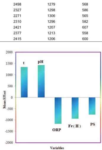
interested variables for each experiment, and m is the number of variables in the model. The calculated values of MEs are represented in the last column of Table 2 and are also plotted in Figure 2. Table 3 represents the correlation matrix for these variables. The value and sign of mean effect demonstrates the relative contribution and direction of influence of each variable on the ferric iron precipitation. As shown in Table 2, the most relevant variables based on their mean effects are pH and leaching temperature. The positive coefficient of these variables mean as the value of this variables increase, the values of ferric iron precipitation increase. These results are in accor-dance with those we have obtained in bioleaching experiments.
Figure 2. Plot of descriptor's mean effects.
Neural network modeling
The next step was the production of ANN and training of it. Input and output data normalization is a significant feature of training the network and per-formed to avoid problems with saturation of the neu-ron transfer function. Input and output data are typi-cally normalized in the range (0,1) or (-1,+1). The type of normalization is problem dependent and may have Table 1. Descriptive statistics of observed and predicted values of ferric iron precipitation (mg/l); EXP refers to experimental; PLS refers to partial least squares; ANN refers to artificial neural network
Set n Minimum Maximum Mean Standard deviation
Training (EXP) 40 317 2514 1282 572
Training (PLS) 40 304 2489 1308 556
Training (ANN) 40 314 2498 1279 568
Prediction (EXP) 20 506 2327 1298 586
Prediction (PLS) 20 381 2271 1306 565
Prediction (ANN) 20 512 2310 1296 582
Validation (EXP) 20 486 2421 1207 607
Validation (PLS) 20 392 2377 1213 558
Validation (ANN) 20 492 2415 1206 600
Table 2. The partial least squares regression coefficients
Variable Notation Coefficient Mean effect
Leaching temperature t 38.75 1345.67
Initial pH pH 732.43 1432.27
Oxidation/reduction potential ORP -2.28 -1173.20
Ferrous iron concentration Fe (II) -1.16 945.13
Particle size PS -8.50 -765.00
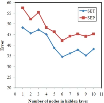
some effects on how well the ANN trains. Here we use Scaled normalization to bring the data into dyna-mic range of the tangent sigmoid transfer function of the network. Before training the ANNs, the parame-ters of network including the number of nodes in the hidden layer, weights and biases learning rates and momentum values were optimized. In order to deter-mine the optimum number of nodes in hidden layer several training sessions were conducted with diffe-rent number of hidden nodes. The values of standard error of training (SET) and standard error of prediction (SEP) were calculated after each 1000 iterations and calculation was stopped when overtraining began, then SET and SEP values were recorded. The recorded values of SET and SEP were plotted against the number of nodes in hidden layer, and the number of hidden nodes with minimum values of SET and SEP was chosen as the optimum one (Figure 3). It can be seen from this figure that 6 nodes in the hid-den layer were sufficient for a good performance of the network. Learning rates of weights and biases and also momentum values were optimized in a simi-lar way and the results are shown in Figures 4-6,
res-pectively. As can be seen, the optimum values of the weights and biases learning rates and momentum were 0.2, 0.2 and 0.3, respectively. The generated ANN was then trained by using the training set for the optimization of weights and biases. However, training was stopped when overtraining began. For the eva-luation of the prediction power of network, trained ANN was used to simulate the ferric iron precipitation included in the prediction set.
Table 4 shows the architecture and specification of the optimized network. After optimization of the net-work parameters, the netnet-work was trained by using training set for adjustment of the weights and biases values by back-propagation algorithm. It is recognized that the neural network can become overtrained. An overtrained network has usually learned completely the motivation pattern it has seen but cannot give precise forecasting for unobserved stimuli, and it would no longer be capable to generalize. There are various methods for overcoming this problem. One method is to utilize a prediction set to assess the pre-diction power of the network during its training. In this method, after each 1000 training iterations, the Table 3. Correlation matrix between selected variables
t pH ORP Fe (II) PS
t 1 -0.029 0.213 -0.124 0.144
pH 1 -0.668 0.750 0.196
ORP 1 -0.642 0.251
Fe (II) 1 -0.097
PS 1
Figure 3. The values of SET and SEP versus number of nodes in hidden layer.
network was used to calculate ferric iron precipitation included in the prediction set. To preserve the predictive power of the network at an enviable level, training was stopped when the value of errors for the prediction set started to increase.
Figure 5. The values of SET and SEP versus biases learning rate.
Figure 6. The values of SET and SEP versus momentum.
The predictive power of the ANN models deve-loped on the selected training sets are estimated on the predictions of validation set chemicals, by cal-culating the q2
that is defined as follow:
− = −
−
2 2
2 ˆ
( )
1
( )
i i
i
y y
q
y y (18)
where yi and ˆyi , respectively are the measured and predicted values of the dependent variable (ferric iron precipitation), y is the averaged value of dependent variable of the training set and the summations cover all the compounds. The calculated value of q was 2 0.996.
Table 4. Architecture and specifications of optimized ANN model
Parameter Value
Number of nodes in the input layer 5 Number of nodes in the hidden layer 6 Number of nodes in the output layer 1
Weights learning rate 0.2
Biases learning rate 0.2
Momentum 0.3 Transfer function (hidden layer) Tangent sigmoid
Transfer function (output layer) Linear
Table 1 shows the descriptive statistics of observed and predicted values of ferric iron precipi-tation for the training, prediction and validation sets. The statistical parameters obtained by ANN and PLS models for these sets are shown in Table 5. The stan-dard errors of training, prediction and validation sets for the PLS model are 180.972, 165.047 and 149.950, respectively, which would be compared with the values of 32.860, 40.739 and 35.890, respectively, for the ANN model. Comparison between these values and other statistical parameters in Table 5 discloses the superiority of the ANN model over PLS ones. The key power of neural networks, unlike regression anal-ysis, is their aptitude to supple mapping of the selected features by manipulating their functional dependence implicitly.
The statistical values of validation set for the ANN model was characterized by q2
= 0.996, R2
= = 0.996 (R = 0.998), 2=
0 0.996
R , 2 =
0.988 m
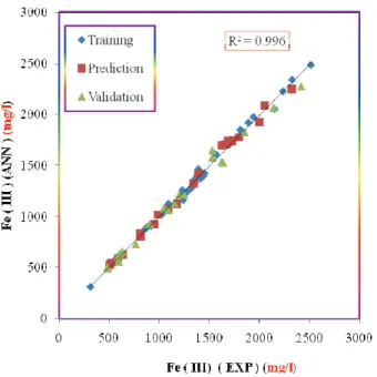
R and k = = 1.002. These values and other statistical parame-ters (Table 5) reveal the high predictive ability of the model. Figure 7 shows the plot of the ANN predicted versus experimental values for ferric iron precipitation ofall of the experiments in data set. The residuals of the ANN calculated values of the ferric iron
precipi-Table 5. Statistical parameters obtained using the ANN and PLS models; R is the correlation coefficient, SE is standard error and F is the statistical F value
Model SET SEP SEV RT RP RV FT FP FV
ANN 32.860 40.739 35.890 0.998 0.997 0.998 10400 3517 4727
tationare plotted against the experimental values in Figure 8. The propagation of the residuals on both sides of the zero line signifies that no systematic error exists in the constructed QSPR model.
Figure 7. Plot of calculated ferric iron precipitation against experimental values.
CONCLUSIONS
Results of this study disclose that ANN can be used successfully in development of a QSPR model to predict the ferric iron precipitation in uranium bioleaching process. Variables appearing in this QSPR model such as leaching temperature, initial pH,
oxidation/reduction potential, ferrous concentration and particle size of uranium ore provide some infor-mation related to different experiments which can affect the ferric iron precipitation. The good agree-ment between experiagree-mental results and predicted values verifies the validity of obtained models. The calculated statistical parameters of these models reveal the superiority of ANN over PLS model. The results show that the ANN model can accurately des-cribe the relationship between the operational condi-tions of bioleaching process and ferric iron precipitation. Nomenclature
QSPR Quantitative structure-property relationship ANN Artificial neural network
PLS Partial least squares ORP Oxidation/reduction potential PS Particle size
R Correlation coefficient
ME Mean effect
t Leaching temperature SE Standard error
F Statistical F value FBR Fluidized bed reactor
W Weight signal
O Output of the node B Bias term
k Slope of regression line EXP Experimental
q Cross validated coefficient SCE Saturated calomel electrode X Predictor (independent) variable Y Response (dependent )variable T Score of X
P Loading of X Q Score of Y S Loading of Y E Residual for X F Residual for Y BP Back-propagation d Distance score SET Standard error of training SEP Standard error of prediction SEV Standard error of validation
REFERENCES
[1] K. Bosecker, FEMS Microbiol. Rev. 20 (1997) 591–604 [2] D. Holmes, Chem. Ind. 1 (1999) 20–24
[3] S. llyas, M.A. Anwar, S.B. Niazi, M.A. Ghauri, B. Ahmad, K.M. Khan, J. Chem. Soc. Pak. 30 (2008) 61-68
[4] G.J. Olson, J.A. Brierley, C.L. Brierley, Appl. Microbiol. Biotechnol. 63 (2003) 249-257
[5] D.P. Kelly, A.P. Wood, Int. J. Syst. Evol. Microbiol. 50 (2000) 511-516
[6] D.E. Rawlings, Annu. Rev. Microbiol. 56 (2002) 65-91 [7] [7] J.A. Brierley, C.L. Brierley, Hydrometallurgy 59 (2001)
233–239
[8] T. Sugio, M. Wakabayashi, T. Kanao, F. Takeuchi, Biosci. Biotechnol. Biochem. 72 (2008) 998–1004
[9] S.M. Mousavi, S. Yaghmaei, M. Vossoughi, A. Jafari, S.A. Hoseini, Hydrometallurgy 80 (2005) 139–144 [10] J.A. Munoz, F. Gonzalez, A. Ballester, M.L. Blazquez,
FEMS Microbiol. Rev. 11 (1993) 109–119
[11] C. Laberge, D. Cluis, G. Mercier, Water Res. 34 (2000) 1145-1156
[12] E. Jorjani, S. Chehreh Chelgani, S.H. Mesroghli, Fuel 87 (2008) 2727–2734
[13] C. Acharya, S. Mohanty, L.B. Sukla, V.N. Misra, Ecol. Model. 190 (2006) 223–230
[14] D. Diamond, D.S. Jyotsna, Res. J. Chem. Sci. 1 (2011) 108-112
[15] Nikhil, B. Özkaya, A. Visa, C.Y. Lin, J.A. Puhakka, O. Yli-Harja, World Academy of Science, Engineering and Technology 37 (2008) 20-25
[16] N.B. Ozkaya, E. Sahinkaya, P. Nurmi, A.H. Kaksonen, J.A. Puhakka, Bioprocess. Biosyst. Eng. 31 (2008) 111– –117
[17] K. Yetilmezsoy, S. Demirel, J. Hazard. Mater. 153 (2008) 1288–1300
[18] N. Daneshvar, A.R. Khataee, N. Djafarzadeh, J. Hazard. Mater. 137 (2006) 1788-1795
[19] E. Sahinkaya, B. Ozkaya, A.H. Kaksonen, J.A. Puhakka, Biotechnol. Bioeng. 97 (2006) 780-787
[20] E. Sahinkaya, J. Hazard. Mater. 164 (2009) 105-113 [21] K. Yetilmezsoy, B. Ozkaya, M. Cakmakci, Neural Network
World 31 (2011) 193-218
[22] K.D. Mehta, B.D. Pandey, T.R. Mankhand, Miner. Eng. 16 (2003) 523–527
[23] M.S. Choi, K.S. Cho, D.S. Kim, H.W. Ryu, J. Microbiol. Biotechnol. 21 (2005) 377-380
[24] D.G. Karamanev, L.N. Nilolov, V. Mamatarkova, Miner. Eng. 15 (2002) 341-346
[25] L. Herrera, P.R. Ruiz, J.C. Aguillon, A. Fehrmann, J. Chem. Tech. Biotechnol. 44 (1989) 171-181
[26] P. Geladi, B.R. Kowalski, Anal. Chim. Acta 185 (1986) 1-17 [27] B.S. Dayal, J.F. MacGregor, J. Chemom. 11 (1997) 73-85 [28] S. Ranar, P. Geladi, F. Lindgren, S.Wold, J. Chemom. 9
(1995) 459-470
[29] A. Lorber, L. Wangen, B.R. Kowalsky, J. Chemom. 11 (1987) 9-31
[30] T. Khayamian, A.A. Ensafi, B. Hemmateenejad, Talanta 49 (1999) 587-596
[31] M. Shamsipur, B. Hemmateenejad, M. Akhond, H. Shar-ghi, Talanta 54 (2001) 1113-1120
[32] A. Hoskuldsson, Chemom. Intell. Lab. Syst. 55 (2001) 23- –38
[33] MATLAB 7.0, The Mathworks Inc., Natick, MA, USA, http://www.mathworks.com
[34] C.M. Bishop, Neural networks for pattern recognition Cla-rendon Press, Oxford, 1995
[35] J. Zupan, J. Gasteiger, Neural Network in Chemistry and Drug Design, Wiley-VCH, Weinheim, 1999
[36] T.M. Beal, H.B. Hagan, M. Demuth, Neural Network Design, PWS, Boston, MA, 1996
[37] J. Zupan, J. Gasteiger, Neural Networks for Chemists: An Introduction, VCH, Weinheim, 1993
[38] T.B. Blank, S.T. Brown, Anal. Chem. 65 (1993) 3081-3089 [39] M. Jalali-Heravi, M.H. Fatemi, J. Chromatogr., A 915
(2001)177-183
[40] A. Golbraikh, A. Tropsha, J. Mol. Graphics. Modell. 20 (2002) 269-276
[41] P.P. Roy, K. Roy, QSAR Comb. Sci. 27 (2008) 302-313 [42] A.G. Maldonado, J.P. Doucet, M. Petitjean, Mol. Divers.
HASSAN GOLMOHAMMADI ABBAS RASHIDI SEYED JABER SAFDARI
Nuclear Science and Technology Research Institute, AEOI, Tehran, Iran
NAUČNI RAD
PREDVI
Đ
ANJE PRECIPITACIJE FERI JONA U
PROCESU BIOLUŽENJA PRIMENOM PARCIJALNIH
NAJMANJIH KVADRATA I VEŠTA
Č
KE
NEURONSKE MREŽE
Razvijena je kvanitativna zavisnost između strukture i svojstava zasnovana na parcijal-nim najmanjim kvadratima i veštačkoj neuronskoj mreži u cilju predviđanja precipitacije gvožđe(III) jona u procesu bioluženja. Ulazne promenljive bile su: temperatura luženja, početni pH, oksido-redukcioni potencijal, koncentracija gvožđe(II) i veličina čestica rude. Izlaz iz modela je bila precipitacija gvožđe(III) jona. Optimalni uslov veštačke neuronske mreže je dobijen podešavanjem različitih parametara metodom probe i greške. Posle optimizovanja i učenja mreže pomoću algoritma sa povratnom propagacijom, generi-sana je neuronska mreža 5-5-1 radi predviđanja precipitacije gvožđe(III) jona. Vrednosti korena srednje kvadratne greške za učenje, predviđanje i validaciju neuronske mreže bile su 32,860; 40,739 i 35,890, redom, koje su manje od onih dobijenih modelom par-cijalnih najmanjih kvadrata (180,972; 165,047 i 149,950, redom). Dobijeni rezultati poka-zuju pouzdanost i dobru prediktivnost neuronske mreže za predviđanja precipitacije gvožđe(III) jona u procesu bioluženja.