International Journal for Quality research UDK- 004.032.26
Original Scientific Paper (1.01)
Vol.4, No. 1, 2010 37
Prasun Das1)1) Indian Statistical Institute SQC & OR Division
203 B. T. Road Kolkata 700108, India
HYBRIDIZATION OF ARTIFICIAL NEURAL NETWORK
USING DESIRABILITY FUNCTIONS FOR PROCESS
OPTIMIZATION
Abstract: As desirability functions, proposed by many authors, follow most of the properties of standard transfer functions used for ANN, the objective of hybridsation in this study is to make use the property of desirability function in the neural network architecture and evaluate their performances while training and optimizing the architecture for an input-output relationship including the concept of composite desirability optimization technique when multiple responses are present. Two important desirability functions, proposed by Harrington, 1965 and Gatza et al., 1972 are used in different combinations with the most useful tan-hyperbolic transfer function using real life data. Three useful hybrid combinations of transfer/desirability functions are observed based on consistent simulation performance, number of nodes and a new measure of composite MSE is proposed here. The work on incorporating the knowledge of composite desirability into ANN architecture and exploiting the non-linearity in inputs versus outputs during normalization is also attempted.
Keywords: Desirability function, Neural network, Transfer function, Hybridisation, Process modeling
1. INTRODUCTION
The quality of a product or service is the set of characteristics, which are defined operationally, often interrelated with different significance and measured in different scale of units. For example, the quality of a steel-rolled product depends on its characteristics like tensile strength, hardness, elongation and so on. Another example could be weight, shape, taste, flavour and the baking quality of biscuits. Some of these characteristics may be interrelated to each other.
The concept of desirability scale arises when there is a need to combine the magnitude of several characteristics to a dimensionless scale (say, d). Generally, this desirability function is so constructed that any property (characteristic) value of a product or service is mapped between zero and one [1]. A desirability scale value of one means the optimum property level of the product or service whereas zero desirability indicates an unacceptable product or service. Any value in between zero and one gives an opportunity to improve the product (or service) quality depending on the closeness to these extreme two points. Harrington, 1965 [1] first defined the desirability function, a slight modification of which was done by Gatza et al. [2] for which the desirability scale can be negative for negative input values. Some different forms of desirability function are also proposed by Derringer et al., 1980 [3].
A composite desirability scale, say D, represents the geometric mean of individual desirability values arising out of several properties. Mathematically, it is
defined as n
n d d d
D = 1. 2.... ………(1)
where, d1, d2, …dn are the desirability values for n properties of the product (or, service)
The geometric mean is taken because in most product development situation, if any one property is so poor that the product is unsuitable for application, then the individual desirability value will be zero and hence the composite desirability will also be zero. On the other hand, the upper bound of D is always one when d1, d2, …dn are all one.
Sometimes, if the product properties are interrelated based on their importance on the final product quality, and then an appropriate power (weight) of each d is considered. The modified composite desirability, as suggested by Derringer, 1994 [4] is then defined as
i n
w w
n w w
d d
d
D = ∑ 1. 2... 2
1 …….….(2)
This modified desirability function, since differentiable, may be used for the optimization process [5]. The use of the method of concurrent optimisation is demonstrated to improve the product quality in a real life industrial manufacturing set-up [6].
some set of processing units that receive inputs from the outside world, which can be referred to appropriately as the ‘input units’ or ‘input nodes’. It does have one or more layers of ‘hidden’ processing units that receive inputs only from the other processing units.
The set of processing units that represent the final result of the neural network computation is designed as the ‘output units’. In the last decade many statisticians have investigated the properties of neural network and it appears that there exists a considerable overlap between statistical and neural network modeling.
There are similarities of terminologies between statistics and neural network like (variables, features), (estimation, learning), (estimates, weights), (interpolation, generalisation); (observations, patterns) and so many [10]. The principal difference between neural networks and statistical approaches is that neural network makes no assumptions about the statistical distribution or properties of the data, and therefore tends to be more useful in business and practical situation.
The purpose of this work is to make an attempt of hybridizing the functional forms desirability functions using their mathematical properties such as continuous, differentiable and boundedness into the neural network architecture in several ways.
This arises since desirability functions follow the same properties of standard transfer functions used in the NN architecture along with the incorporation of the concept of composite desirability while modeling the process for its control and optimization through neural network analysis.
2. TRANSFER FUNCTION AND
DESIRABILITY FUNCTION
Transfer Functions
It is used to calculate the output response of a neuron. The sum of the weighted input signal (net input) is applied with an activation to obtain the response. For neurons in the same layer, same transfer functions are used. The non-linear transfer functions are used in a multiplayer net. The transfer functions may be simply non-negative identity function, step function, ramp function, sigmoid etc. Transfer function whose outputs saturate (e.g. f(x) = 1 and f(x) = 0 as x tends to ∝ and –
∝ respectively) are of great interest in all neural network modeling. Inputs to a neuron that differs very little are expected to produce approximately the same output, which justifies using continuous node function. Another property of transfer function is that it should be differentiable for implementing different learning algorithms. These functions typically fall into one of three categories: linear, threshold and sigmoid. For linear units, the output activity is proportional to the total weighted output. For threshold units, the output are set at one of two levels, depending on whether the total input is greater than or less than some threshold value. For sigmoid units, the output varies continuously but not linearly as the input changes. Sigmoid units bear a greater resemblance to real neurons than do linear or threshold units, but all three must be considered rough approximations. A list of few important transfer functions commonly used in network architecture is shown below.
Figure 1 - Standard Transfer Functions for NN Architecture
The hard-limit transfer function limits the output of the neuron to either 0, if the net input argument n is less than 0; or 1, if n is greater than or equal to 0. The purelin (linear) transfer function produces the output (a) of the neuron equal to the net input argument n. The log-sigmoid transfer function takes the input, which may have any value between plus and minus infinity, and squashes the output into the range 0 to 1.
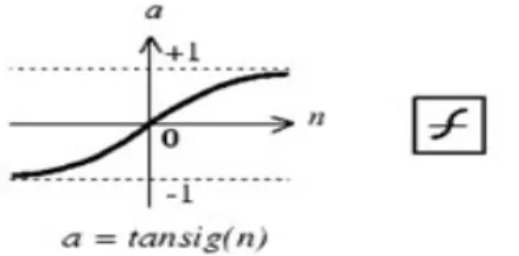
Tan-Sigmoid Transfer Function
The graph of the tan-sigmoid transfer function is shown below.
This function approaches its bounds –1 and +1, different from the earlier functions discussed, more quickly than others. The functional form of this transfer
function is n n n n
e
e
e
e
a
− −+
−
=
…………..(3)
Desirability Function
, proposed by
Harrington (1965)x e
e
y
=
− − , for one sided specification…..(4)The value of y varies from 0 to 1 and it is differentiable except y = -1. Using this desirability function a transfer function named ‘Harring’ and a derivative function of above desirability function named ‘dHarring’ has been constructed for use in this work. The form of derivative function is otherwise y where y y e e dx dy
D x x
, 0
0 ,
ln
. exp( )
= > − = − = = − − − ..(5)
Desirability function, proposed by Gatza & McMillan (1972) 1 1
1
− − −−
−
=
−e
e
e
y
x e ………..(6)This is a modification of Harrington’s function, which produces negative values of desirability for unacceptable properties. Using this desirability function a transfer function named ‘Gatza’ and a derivative function of above desirability function named ‘dGatza’ has been constructed here. The form of derivative function is
(
)
{
}
{
(
)
}
[
]
otherwise e e y if e e e y x e e y dx dy D , 0 1 , 1 1 ln 1 1 1 1 1 1 1 1 = − − > − + − − + − = = − − − − − − − …...(7)3. AN APPROACH OF HYBRIDIZATION
The overall aim of this work is to make use the property of desirability function in the neural network architecture and evaluate their performances as a hybrid neural network model while training and optimising the architecture for a complex, non-linear input-output relationship including the concept of composite desirability optimisation technique when multiple responses are present.
Since desirability functions follow most of the properties of standard transfer functions used for ANN like bounded between zero and one and differentiable, the concept of hybridsation develops. In this work, two desirability functions would be used in different combinations with the existing transfer function for training and optimising the architecture using real-life process data. The functional forms of their derivatives are therefore required to use the gradient-based training algorithm; either scaled conjugate gradient (SCG) or
Levenberg-Marquardt optimization. The corresponding programs for desirability functions are written in MATLAB and used later as a transfer function while training.
In the second stage of the study, concept and formula of composite desirability optimisation is hybridised in the neural network model, the architecture is customarily designed and then an attempt was undertaken to evaluate its performance on multiple responses from another set of process data.
The plan of study is therefore formulated as follows.
Step-1. Fixing a 2-layer architecture, for training using different combinations of existing transfer function and the new ones based on desirability functions, as proposed by Harrington and Gatza.
Step-2. Evaluating the performance of different combinations of transfer functions based on simulating (testing) the architectures and then attempting to optimise those with respect to mean square errors.
Step-3. Normalizing the database using the bounded property of desirability function and then comparing the performances of network training with the results when usual ‘minimax normalization’ is done.
Step-4. Choosing the best alternative desirability function as transfer function and incorporating them in the ANN architecture to optimise multiple responses using composite desirability optimisation criteria.
4
. PROCESS INFORMATION –
VARIABLES FOR ANN
For the first phase of study, data were considered with the objective of robust control of fermentation process. The fermentation process is a biological base system that runs smoothly depending on effective operator supervisory and formulated rules from knowledge based systems (Lennox, [11]). However, maintaining consistency of growth pattern over the batches of commercial yeast production through addition of water, molasses and other chemicals creates problem to the manufacturer. The data used in this context is obtained from an industry producing baker’s yeast. Relevant information on fermenter parameters [Air CFM, Temp, pH, Dip (M), Vol(L), Amps, ALC %, Spin], Yeast in fermenter (kg., increment, G.M.), Wort and other chemical additions are collected from Brew sheet for consecutive batches of yeast production.
The input parameters and corresponding output characteristics were selected first. There is a total of 16 time sequences (hours of production) for a particular batch of yeast fermentation. The necessary collected information on complete batch operation with selected parameters for analysis is given below.
1)Time sequence: X1
3)Temperature for this interval: X3
4)PH of the liquid at the start of the sequence: X4 5)Alcohol (%) of the liquid at the start of the
sequence: X5
6)Residual sugar at the start of the sequence: X6
7)% Increase of yeast at the end of the time sequence: Y
A total of 800 observations, equivalent to 24 batches, on the above parameters are collected. The ranges of the variables used in this work are as follows.
Table 1. Summary Statistics of Variables Sl. No. Variable description Coded
variable
Unit Minimum (Xmin)
Maximum (Xmax)
1 Time sequence X1 -- 1 16
2 Airflow rate X2 CFM 2000 4000
3 Temperature X3 0C 30.75 36.42
4 pH X4 -- 4.040 5.235
5 Alcohol X5 % 0.087 0.190
6 Residual Sugar X6 Kg. 97.00 1069.00
7 % Increase of yeast Y % 1.64 24.71
Each variable (say, Xi) is normalized within the range of 0 to 1 for ANN modeling by the “minimax normalization” technique as
min max
min X X
X X
X N −
−
= …………(8)
where XN is the normalized value of the variable Xi, X is the actual value and Xmax and Xminare the maximum
and the minimum values of Xi, respectively.
In the second stage of the study, data were considered from steel product rolling process. In metal formation of steel, material property during formation depends primarily on the number of constituents, some of which are controllable and others are not. The necessary constituents considered here are given below.
Table-2. Summary Statistics of Variables
Sl. No Variables Coded from in Equation
Lower Boundary
Upper
Boundary Units
1 Pearlite X1 0 35 Frac..%
2 Manganese X2 0.25 1.5 Wt. %
3 Silicon X3 0 0.4 Wt. %
4 Phosphorus X4 0 0.05 Wt. %
5 Tin X5 0 0.2 Wt. %
6 Free Nitrogen X6 0.005 0.024 Wt. %
7 Sulphur X7 10 40 μm
The response variables and their relationship with the constituents (obtained from the prior knowledge in materials science) considered in this work are given below.
Uniform Elongation, Y1 = 0.27 – 0.16 * X1- 0.015*
X2 – 0.04* X3 – 0.043 *X5 – 1.1* X6.
Flow Stress at 0.2 % strain, Y2 = 15.4 * (16 +0.27 *
X1 + 2.9* X2 + 9* X3 + 60* X4 + 11* X5 + 244*X6 + 0.97/sqrt(X7))…………(9)
Data were generated based on these two equations.
5. RESULTS AND INTERPRETATION
A multilayered feed-forward fully connected network 6-N1-N2-1 is considered, where the number of input variables (neurons) is six, N1 and N2 being the number of neurons in the two hidden layers and %growth (Y) of yeast is considered as the single
output variable. The tan-sigmoid function is used as a standard transfer function in one of the hidden layers while Purelin transfer function is used at the output layer only. The two hidden layers of the architecture have been varied with the 9 transfer function combinations as ‘tansig-tansig’,‘tansig-Harring’,‘tansigGatza’,‘Harring-tansig’,‘Gatza-tansig’, ‘Harring-Gatza’, ‘Gatza-Harring’,‘Harring-Harring’ and ‘Gatza-Gatza’.
networks are trained with supervised LM algorithm. The learning parameter and the momentum parameter are kept fixed at their default values. The maximum epochs is set at 600.
For each of the above transfer functions combination, a set of 21 architectures has been considered by varying the number of hidden neurons in the two hidden layers, starting from (6-1-1-1) to (6-6-6-1), thus increasing total number of hidden nodes from 2 to up to 12. For each architecture, a sample of 10 train-MSE has been observed with a maximum number of
600 epochs each. The average and standard deviation of these 10 samples are given for each architecture under each transfer function combination (see Annesure-1) along with the overall averages. All these trained networks are used to simulate (test) over rest 20% data in the same manner and the subsequent statistics of simulation study have also been illustrated in Annexure-1. The plots of average train MSE and test MSE versus the number of hidden nodes, considering all the 21 architectures are shown in Figure-3 for each of the 9 combinations of transfer functions.
TF Com bination: tansig-tansig
0 1 2 3
2 4 5 6 6 7 8 8 9 10 12
# hidden nodes
Av
g
. M
S
E
train MSE test MSE
TF Combination: tansig-Harring
0 1 2 3
2 4 5 6 6 7 8 8 9 10 12
# hidden nodes
Av
g
. M
S
E
train MSE test MSE
TF Combination: tansig-Gatza
0 0,51 1,52 2,53 3,54
2 4 5 6 6 7 8 8 9 10 12
# hidden nodes
Av
g
. M
S
E
TF Com bination: Harring-tansig
0 1 2 3
2 4 5 6 6 7 8 8 9 10 12
# hidden nodes
Av
g
. M
S
E
train MSE test MSE
TF Combination: Gatza-tansig
0 1 2 3
2 3 4 4 5 5 6 6 6 7 7 7 8 8 8 9 9 10101112
# hidden nodes
Av
g
. M
S
E
train MSE test MSE
TF Com bination: Harring-Gatza
0 5 10
2 4 5 6 6 7 8 8 9 10 12
# hidden nodes
Av
g
. M
S
E
train MSE test MSE
TF Combination: Gatza-Harring
0 2 4 6
2 4 5 6 6 7 8 8 9 10 12
# hidden nodes
Av
g
. M
S
E
TF Comb inatio n: Harrin g- Harring
0 2 4 6
2 3 4 4 5 5 6 6 6 7 7 7 8 8 8 9 9 10 1 0 11 1 2 # hidden nodes
Av
g
. M
S
E
train MSE test MSE
TF Combination: Gatza-Gatza
0 1 2 3 4 5 6 7 8
2 3 4 4 5 5 6 6 6 7 7 7 8 8 8 9 9 10101112
# hidden nodes
Av g . M S E train MSE tes t MSE
Figiure 3 Training performances for different combination of transfer functions
The overall summary statistics for each of the 9 combinations of transfer functions are given below. Table-3. Overall Summary Statistics of Mean Square Error (MSE)
Combinations of Transfer Functions
N = 21 (experimental architectures) ta nsig -ta nsig ta nsig
-Harring ta
nsig -Ga tza Harring- ta nsig Ga tza -ta nsig H a
rring-Gatza Gatza- Harring Harring- Harring Gatza- Gatza
Training
Average 1.2403
91 1.2421 69 1.2904 29 1.2698 64 1.2837 7 1.3020 67 1.3465 59 1.2705 33 1.3140 91
Std. Dev. 0.0687
03
0.0853 65
0.2197
06 0.1979
0.1926 62 0.2000 69 0.7218 34 0.0922 07 0.1944 26
Minimum 0.9241
83 (6-6) 0.9493 49 (6-6) 0.9676 (6-6) 0.9320 88 (6-6) 0.9826 69 (6-6) 1.0232 96 (6-5) 1.0209 35 (6-5) 0.9579 07 (6-6) 1.0254 51 (6-5)
Maximum 1.6539
(1-1) 1.6534 (1-1) 1.6501 4 (1-1) 1.6692 7 (1-1) 1.6577 9 (1-1) 1.6440 6 (1-1) 2.5087 4 (3-1) 1.6512 (1-1) 1.7259 7 (3-1) Testing
Average 1.8568
37 6.7434 47 1.9846 66 19.784 62 8.7062 78 19.094 99 65.324 88 580.09 08 12.788 14
Std. Dev. 1.0810
26 63.949 86 1.2114 37 210.62 88 97.327 54 159.84 13 819.68 2 7053.4 75 155.56 89 Best (Minimum) 1.4275 2 (6-1) 1.6079 8 (3-3) 1.4973 7 (4-2) 1.4470 8 (4-4) 1.5509 (6-2) 1.4821 7 (5-1) 1.5057 9 (4-3) 1.4990 6 (4-4) 1.4772 6 (4-1)
Worse – 1
2.5202 (4-1) 2.6969 7 (6-2) 2.7005 6 (5-4) 2.7543 4 (6-6) 2.5010 2 (5-3) 41.847 66 (6-2) 3.2031 3 (5-4) 131.03 18 (4-2) 3.5541 (3-3)
Worse – 2
The following observations are made from Table 2. 1.Minimum and Maximum train MSE, out of 21
architectures, were observed mostly in case of minimum (1-1) and maximum (6-6) number of hidden nodes of an architecture, except the cases like (3-1) and (6-5). This is expected since, in general, train MSE decreases with the increase in number of nodes for architecture.
2.Considering test MSE of 21 architectures, average and standard deviations were estimated for each of transfer function combinations selected for this study. It is observed that the average levels are quite low for two combinations, tansig-tansig (1.856837) and tansig-Gatza (1.984666) respectively. The performance of testing is also quite consistent (1.081026 and 1.211437 respectively) for these two combinations over all the 21 architectures selected.
3.For each of the transfer function combinations, the optimum architecture was found based on the minimum test MSE. The total number of hidden nodes is varying from 5 (4-1) to 8 (4-4, 6-2). 4.The last three worse situations of testing MSEs
were tabulated along with the respective architectures to see the extent of skewness for test MSE values from a set of over 21 observations. In two cases, Harring-Gatza and Harring-Harring, the first worse situation itself is starting from a test MSE value of 41.84766 and 131.0318 respectively, which are definitely unacceptable.
The following table arranges the transfer function combination, the best architecture and its total hidden nodes based on minimum test MSE in ascending order of magnitude.
Table-4. Comparison of TF-combinations based on MSEs and Nodes
Sl No.
TF-combination test mse train mse architecture # hidden nodes
Remarks
1. tansig-tansig 1.42752 1.17579 (6-6-1-1) 7 test MSE(ref. Table-2 more consistent )
2. Harring-tansig 1.44708 1.21092 (6-4-4-1) 8 More nodes, Inconsistent test MSE (ref. Table-2) 3. Gatza-Gatza 1.47726 1.38414 (6-4-1-1) 5 Minimum nodes
4. Harring-Gatza 1.48217 1.29296 (6-5-1-1) 6 Inconsistent, highly skewed
(ref. Table-2)
5. tansig-Gatza 1.49737 1.31403 (6-4-2-1) 6 test MSE(ref. Table-2 more consistent )
6. Harring-Harring 1.49906 1.2084 (6-4-4-1) 8 Inconsistent, highly skewed (ref. Table-2)
7. Gatza-Harring 1.50579 1.27253 (6-4-3-1) 7 More nodes, Inconsistent
test MSE (ref. Table-2)
8. Gatza-tansig 1.5509 1.16184 (6-6-2-1) 8 More nodes
9. tansig-Harring 1.60798 1.29852 (6-3-3-1) 6 High MSEs
We now combine both train and test MSE by assigning weights to get a composite measure of MSE. Each weight (wi) strictly lies between 0 and 1. Further, the weight on test MSE will be greater or equal to the weight on train MSE. This is because test MSE is more important than train MSE while simulating any process using a particular trained and optimised architecture. Moreover, train MSE is more consistent than test MSE. We, thus, define a composite measure of MSE as.
∑
=> ≥ >
+ =
1 , 0 1
, ) ( * ) ( *
2 1
2 2
2 1
i
w w w
MSE train w MSE test w MSE
Composite ……(10)
Using equation (6), we take five combinations of (w1,
Table-5. Comparison of Composite MSE for different weight combinations Weights: (w1, w2) Sl
No. TF-combina
tion test mse
train
mse (0.5,0.5) (0.6,0.4) (0.7,0.3) (0.8,0.2) (0.9,0.1) Average Range
1.
tansig-tansig
1.427 1.175 1.308 1.333 1.357 1.381 1.404 1.356 0.097
2.
Harring-tansig
1.447 1.210 1.334 1.358 1.380 1.403 1.425 1.380 0.091
3.
Gatza-Gatza
1.477 1.384 1.431 1.441 1.450 1.459 1.468 1.450 0.037
4.
Harring-Gatza
1.482 1.292 1.391 1.410 1.428 1.446 1.464 1.428 0.074
5.
tansig-Gatza
1.497 1.314 1.409 1.427 1.445 1.463 1.480 1.445 0.071
6.
Harring-Harring
1.499 1.208 1.362 1.390 1.418 1.446 1.473 1.418 0.111
7.
Gatza-Harring
1.505 1.272 1.394 1.417 1.440 1.462 1.484 1.439 0.090
8.
Gatza-tansig
1.550 1.161 1.370 1.408 1.445 1.481 1.516 1.444 0.146
9.
tansig-Harring
1.607 1.298 1.461 1.492 1.522 1.551 1.580 1.521 0.118
The following table summarises the reasons for choice of optimum transfer function combination along with a particular architecture.
The last column indicates the ranking for choice where rank-1 indicates the best choice.
Table-6. Summary for choice of TF-Combinations Sl
No.
TF-combination architecture # hidden nodes
Remarks Ranking (Optimum
Choice)
1. tansig-tansig (6-6-1-1) 7 test MSE most consistent (ref.
Table-2) 3
2. Harring-tansig (6-4-4-1) 8 More nodes, Inconsistent test
MSE (ref. Table-2) 5 3. Gatza-Gatza (6-4-1-1) 5 Minimum nodes, composite
MSE most consistent 2 4. Harring-Gatza (6-5-1-1) 6 Inconsistent, highly skewed
(ref. Table-2) 8
5. tansig-Gatza (6-4-2-1) 6
test MSE more consistent (ref. Table-2), composite MSE more consistent
1
6. Harring-Harring (6-4-4-1) 8
Inconsistent, highly skewed test MSE (ref. Table-2),
more nodes
9
7. Gatza-Harring (6-4-3-1) 7 More nodes, Inconsistent test
MSE (ref. Table-2) 7 8. Gatza-tansig (6-6-2-1) 8 More nodes, composite MSE
inconsistent 4
9. tansig-Harring (6-3-3-1) 6 High MSEs, composite MSE
From the above table (Table-5), the following three transfer function combinations are selected for next phase of study.
1.tansig-Gatza-purelin 2.Gatza-Gatza-Purelin 3.tansig-tansig-Purelin
The tansig-tansig-purelin combination is chosen to compare the performance with other two combinations where Gatza’s desirability function is used as a transfer function in the neural network architecture.
6. SOME EXPERIMENTAL CASES
Case-1. Normalization technique (data: Steel Rolling Process)
The objective of investigation, using the non-linearity and bounded property of Harrington’s desirability function, was to compare the performance of training when
• normalization of input and output observations is done using desirability function instead of minimax normalization; and
• normalization of input observations only is done using desirability function instead of minimax normalization
The result on MSE values in both the cases, when desirability function was used for normalization, as explained above, was found inferior than the results in case of minimax normalization process. So, any comment on the betterment of normalization process using desirability function cannot be made at this point. The possible explanation could be that the data for both the responses (uniform elongation and Flow Stress) have been generated using linear equations except (see Section 4.0) one input variable which is inversely proportional to square of the response, hence minimax normalization (which is a linear transformation of the data) might be giving better result in terms of input-output mapping.
Case-2. Custom Network (data: Fermentation Process)
The design of the feed forward network is as follows:
For each input variable (node), it is connected to a single node only in the first hidden layer and in this layer desirability function is used as transfer function. Outputs from this hidden layer are fully connected to the next layer. The tan-sigmoid transfer function is used for the other layers. The architecture is shown in Figure-4.
Figure 4. Schematic Diagram of a Custom Network
The normalization of the data is done using minimax normalization technique. The data represent six input variables and one response variable from fermentation process.
The results of MSEs using the two important desirability functions through custom designed network are shown in Table-7.
It is observed from the above table that the
Table-7. Comparison of MSEs based on desirability functions (Network: Custom) Desirability
functions. Gatza Harrington tansig
Train MSE Test MSE Train MSE Test MSE Train MSE Test MSE 1.7163 1.5743 1.8032 1.6941 1.6623 1.7218 1.7287 1.6305 1.8239 1.5926 1.6676 1.7294 1.7751 1.6384 1.7484 1.5692 1.681 1.7502 4.8824 4.3504 2.6521 2.1326 1.6697 1.734 3.6456 3.0067 1.7028 1.5207 1.6718 1.7472 4.8265 3.9674 1.9667 1.7946 1.7709 1.7988 1.6399 1.4355 1.8806 1.7339 1.6576 1.7043 7.8295 6.5411 2.0535 1.8708 1.6654 1.7338 1.5695 1.3175 1.9116 1.7601 1.6923 1.7627 6-1-1
8.0943 7.0217 1.9391 1.857 1.6688 1.7357 Average MSE 3.77078 3.24835 1.94819 1.75256 1.68074 1.74179
1.8709 2.1231 4.1467 5.4755 4.3546 4.1116 1.6348 1.8775 1.6233 2.0413 1.6686 1.7048 1.6402 1.8771 1.701 2.0479 1.6751 1.6909 5.0273 5.7502 1.612 2.0137 1.6434 1.7579 3.0927 3.6219 1.6942 2.044 1.6619 1.7338 5.0069 5.2639 1.6179 2.0431 1.6928 1.6866 1.8931 2.1592 1.6354 2.0495 1.6778 1.7285 3.5847 3.9352 1.7666 2.1393 1.7036 1.7487 1.6538 1.917 1.6503 2.0957 1.6627 1.7232 4-2-1
14.263 19.977 1.7272 2.0838 1.6742 1.7275 Average MSE 3.96674 4.85021 1.91746 2.40338 1.94147 1.96135
Case-3. Composite Desirability (data: Steel Rolling Process)
The approach adopted to incorporate the concept of composite desirability in the neural network architecture was thought as follows:
Approach-A:
Step-1. Generate the database based on simple linear regression equations between (X,Y);
Step-2. Find out the desirability values for all the output variables, using desirability functions for each of the output variables;
Step-3. Find out the composite desirability (D) after combining the desirability values for all the variables;
Step-4. Train the architecture between (X,D); Step-5. Simulate the trained architecture;
Step-6. Store predicted composite desirability values.
Approach-B:
Repeat from Step-1 to Step-3 as earlier. Step-4. Train the architecture between (X,Y); Step-5. Simulate the trained architecture;
Step-6. Find out desirability of all variables of simulated output and then find out composite desirability by combining these;
Step-7. Store this predicted composite desirability values.
It is observed that the second approach performs better in terms of MSE of composite desirability values.
7. CONCLUSION
Optimization of product features necessarily needs optimization of the associated process parameters. Modeling of process data often becomes the pre-requisite. This is done in many ways, however validation of the developed model is very much required in order to use it in future. The accuracy and precision for prediction and optimization depends on the relationship among them. Neural network technique helps in developing some complex relationship and also becomes helpful when nothing is known about the true behaviour of process parameters and product characteristics.
important desirability functions, proposed by Harrington, 1965 and Gatza et al., 1972 are considered along with the most useful tan-sigmoidal transfer function. Altogether nine combinations of these three functions were tried on two hidden layered network consisting of six input variables and one output variable. Based on 21 different architectures used for each of the nine combinations, the three hybrid transfer function combinations, namely, tansig-Gatza, Gatza-Gatza and tansig-tansig are observed performing uniformly better than others based on consistent simulation performance, number of nodes and a new measure of composite MSE developed in this work.
These findings definitely help us not to restrict ourselves in selecting the appropriate transfer functions from the available list but to think about developing some new ones depending on the process knowledge in order to increase the efficiency of network optimization. The other use of desirability function for normalization of input and/or output data, due to its bounded ness property along with its effect on non-linearity, is not really established through this study. However, some prior knowledge towards the nature of individual input-output relationship based on the relevant process technology would definitely guide in using proper
desirability function for normalization of data and accordingly it would increase the efficiency of the designed network. The concept of incorporating composite desirability into ANN architecture was also attempted.
8. FUTURE SCOPE
The concept of composite desirability to convert multiple responses into a single response using various desirability functions with suitable properties can be used to extract the subject knowledge corresponding to complex input-output relationship through optimization of custom design neural network architecture. The solution space, thus obtained, can be searched for augmentation of process knowledge and compared with the results when the concept of composite desirability is not considered inside the architecture. The proper choice of desirability function into ANN architecture, instead of existing transfer functions, can always be a research topic of interest based on the knowledge of application domain.
REFERENCES:
[1] E.C. Harrington Jr., (1965), The desirability Function, Industrial Quality Control, April, pp. 494-498 [2] P.E. Gatza and R.C. McMillan, (1972), The use of experimental design and computerized data analysis
in Elastomer Development Studies, Division of Rubber Chemistry, American Chemical Society fall meeting, Paper No. 6, Cincinnati, Ohio, October, pp. 3-6
[3] G.C. Derringer, and R. Suich, (1980), Simultaneous optimization of several response variables, Journal of Quality Technology, 12 (4), October, pp. 214-219
[4] G.C. Derringer, (1994), A balancing act: optimizing a product’s properties, Quality Progress, June, pp. 51-58
[5] E. Del Castillo, D.C. Montgomery, D. McCarville, (1996), Modified desirability functions for multiple response optimization, Journal of Quality Technology, 28 (3), July, pp. 337-345
[6] P. Das, (1999), Concurrent optimization of product performance characteristics using multiple desirability functions, Quality Engineering, 11 (3), March, pp. 365 – 368
[7] S. Haykin, (1994), Neural Networks: A Comprehensive Foundation, McMillan, NY.
[8] A. Nigrin, (1993), Neural Networks for Pattern Recognition, Cambridge, The MIT Press, MA. [9] J. M. Zurada, (1992), Introduction To Artificial Neural Systems, Boston: PWS Publishing Company [10]W. S. Sarle, (1994), Neural Networks and Statistical Methods, Proceedings of the Nineteenth Annual
SAS Users Group International Conference
ANNEXURE-1
Architecture Optimisation: Summary of 10 Performances, each with Max. 600 Epochs - During Training
Tansig-tansig Tansig-Harring Tansig-Gatza Harring-tansig Gatza-tansig Archit.
Average Std Dev Average Std Dev Average Std Dev Average Std Dev Average Std Dev
(1-1-1) 1.6539 0.007616 1.6534 0.005418 1.65014 0.02391 1.66927 0.036693 1.65779 0.000553
(2-1-1) 1.52737 0.036204 1.53893 0.084203 1.5145 0.080739 1.58961 0.06624 1.54484 0.05253
(2 2 1) 1.50477 0.083695 1.47509 0.096426 1.49231 0.085659 1.53254 0.101602 1.48172 0.084215
(3 1 1) 1.47832 0.085654 1.42706 0.050091 1.4822 0.125549 1.42672 0.044472 1.44305 0.040671
(3 2 1) 1.37184 0.033442 1.41417 0.115184 1.41872 0.072895 1.38403 0.056685 1.38231 0.04835
(3 3 1) 1.2969 0.034553 1.29852 0.088652 1.36483 0.078866 1.29928 0.054732 1.35219 0.081191
(4 1 1) 1.36144 0.038638 1.34912 0.116911 1.34598 0.095931 1.35264 0.120146 1.64135 0.79466
(4 2 1) 1.28253 0.057825 1.31396 0.047102 1.31403 0.067475 1.34773 0.133379 1.32643 0.056028
(4 3 1) 1.25165 0.070452 1.20405 0.046767 1.258 0.113809 1.26781 0.115095 1.22998 0.066956
(4 4 1) 1.18743 0.10851 1.19568 0.053094 1.21239 0.095607 1.21092 0.111943 1.216 0.097706
(5 1 1) 1.22586 0.070926 1.2733 0.078813 1.28705 0.148693 1.55162 0.829883 1.30592 0.130974
(5 2 1) 1.22583 0.052856 1.26734 0.182024 1.29222 0.119169 1.20299 0.042025 1.28662 0.082107
(5 3 1) 1.16677 0.041517 1.13548 0.061679 1.25144 0.152122 1.18953 0.092048 1.21158 0.098547
(5 4 1) 1.09454 0.048083 1.043239 0.053095 1.19731 0.110398 1.130551 0.075256 1.10747 0.082092
(5 5 1) 1.088456 0.098459 1.06521 0.056843 1.109243 0.089118 1.036461 0.070395 1.121177 0.17125
(6 1 1) 1.17579 0.039057 1.17482 0.075834 1.21515 0.040871 1.22418 0.091961 1.26836 0.114118
(6 2 1) 1.12903 0.122898 1.19407 0.112171 1.15826 0.057827 1.17782 0.079393 1.16184 0.061747
(6 3 1) 1.13017 0.123771 1.100941 0.069738 1.366544 0.898258 1.07496 0.073509 1.13014 0.091077
(6 4 1) 1.016114 0.032647 1.044961 0.056285 1.081238 0.131227 1.052597 0.056494 1.051807 0.059276
(6 5 1) 0.955314 0.051013 0.966864 0.067084 1.119848 0.142714 1.0138 0.047805 1.055918 0.072165
(6-6-1) 0.924183 0.048526 0.949349 0.109643 0.9676 0.08402 0.932088 0.070737 0.982669 0.082937
Total 26.04821 0.099123 26.08555 0.153031 27.099 1.013683 26.66715 0.822455 26.95916 0.779492 Average 1.240391 0.068703 1.242169 0.085365 1.290429 0.219706 1.269864 0.1979 1.28377 0.192662
During Simulation
Tansig-tansig Tansig-Harring tansig-Gatza Harring-tansig Gatza-tansig
Archit.
Average Std Dev Average Std Dev Average Std Dev Average Std Dev Average Std Dev
(1-1-1) 1.79412 0.035855 1.79932 0.021989 1.80718 0.094876 1.72976 0.1503 1.77741 0.000644
(2-1-1) 1.6738 0.107443 1.74469 0.070149 1.76207 0.101467 1.61503 0.212051 1.6767 0.101328
(2 2 1) 1.58308 0.120163 1.79176 0.391451 1.68142 0.133236 1.6358 0.182369 1.5909 0.131459
(3 1 1) 1.64338 0.092449 1.68172 0.062914 1.63129 0.140613 1.4808 0.161981 1.6342 0.080472
(3 2 1) 1.52405 0.088644 1.65427 0.080011 1.83794 0.803676 1.5171 0.132432 1.56747 0.118668
(3 3 1) 1.58786 0.151726 1.60798 0.351827 1.72078 0.292496 1.46967 0.156173 1.86059 0.598503
(4 1 1) 2.5202 2.83612 1.77586 0.215498 1.65633 0.175105 1.55801 0.193903 1.84186 0.884298
(4 2 1) 1.5358 0.165272 1.85133 0.812811 1.49737 0.134533 1.55785 0.166689 142.4796 445.8181
(4 3 1) 1.68178 0.208719 2.64551 3.526395 1.89181 0.956334 1.69276 0.46279 1.5843 0.228212
(4 4 1) 1.70818 0.19962 1.68757 0.296838 1.93119 0.794307 1.44708 0.126231 1.60136 0.164088
(5 1 1) 1.57843 0.217373 1.91448 0.928462 1.69869 0.585044 2.01444 0.920922 1.61467 0.220944
(5 2 1) 1.59759 0.193367 1.84042 0.464668 1.64246 0.227197 1.64488 0.258372 1.59078 0.207762
(5 3 1) 1.58813 0.08678 1.87915 0.429774 1.70924 0.523264 86.71595 268.9148 2.50102 2.71114
(5 4 1) 1.73214 0.225651 1.86292 0.435516 2.70056 3.101447 295.5158 926.9995 1.73847 0.218009
(5 5 1) 2.47858 1.743109 2.20497 1.094778 2.96986 2.554504 1.72822 0.380523 1.68606 0.202131
(6 1 1) 1.42752 0.117683 2.02961 1.046245 1.81934 1.106753 1.5058 0.132459 2.15038 1.580127
(6 2 1) 1.51109 0.201131 2.69697 3.49137 1.54966 0.427205 1.92919 0.924346 1.5509 0.196463
(6 3 1) 2.14022 1.23203 9.12593 17.43431 2.22326 1.490677 1.57908 0.146258 2.38426 2.377771
(6 4 1) 2.82942 2.44713 95.01722 292.4804 1.8977 0.655814 2.61237 1.465908 1.97761 0.627958
(6 5 1) 2.17608 0.889523 2.14854 0.415095 3.65342 2.633132 1.77316 0.272712 1.93967 0.419887
(6-6-1) 2.68212 2.187822 2.65217 1.710316 2.39642 0.794657 2.75434 2.527126 6.08367 12.42379
ANNEXURE-1
Architecture Optimisation: Summary of 10 Performances, each with Max. 600 Epochs - During Training
Harring-Gatza Gatza-Harring Harring-Harring Gatza-Gatza
Archit.
Average Std Dev Average Std Dev Average Std Dev Average Std Dev
(1-1-1) 1.64406 0.028624 1.6576 9.43E-05 1.6512 0.013519 1.71571 0.000975 (2-1-1) 1.54167 0.06735 1.52009 0.018907 1.59541 0.06727 1.57165 0.073608
(2 2 1) 1.49972 0.077035 1.51023 0.102944 1.51355 0.092031 1.56245 0.104348
(3 1 1) 1.47073 0.109483 2.50874 3.183885 1.51875 0.089011 1.72597 0.773743
(3 2 1) 1.38063 0.104313 1.38186 0.025512 1.381688 0.064254 1.45367 0.101832
(3 3 1) 1.40962 0.111811 1.41132 0.11104 1.33569 0.077955 1.39757 0.084701
(4 1 1) 1.39957 0.121525 1.36603 0.045519 1.39667 0.138044 1.38414 0.08145
(4 2 1) 1.37826 0.075506 1.36278 0.073004 1.27188 0.081232 1.38504 0.101492
(4 3 1) 1.32789 0.107713 1.27253 0.061672 1.30288 0.144029 1.26026 0.083171
(4 4 1) 1.25133 0.076646 1.20647 0.079341 1.2084 0.093962 1.21684 0.066215
(5 1 1) 1.29296 0.064821 1.54572 0.821159 1.28414 0.121101 1.35105 0.13092
(5 2 1) 1.29118 0.160678 1.30797 0.137624 1.23161 0.045493 1.26297 0.116049
(5 3 1) 1.24853 0.137165 1.22805 0.12349 1.1886 0.112323 1.241 0.177901
(5 4 1) 1.08713 0.048819 1.12329 0.056409 1.12797 0.074405 1.18108 0.097361
(5 5 1) 1.070726 0.067511 1.080656 0.067228 1.174 0.065944 1.086535 0.123229
(6 1 1) 1.50919 0.799605 1.24307 0.080182 1.16073 0.083584 1.215 0.055831
(6 2 1) 1.17544 0.093662 1.20526 0.08434 1.20555 0.146108 1.168 0.109626
(6 3 1) 1.13932 0.071081 1.17711 0.08853 1.16728 0.107586 1.26785 0.132116
(6 4 1) 1.1779 0.144294 1.124575 0.06784 1.037812 0.049804 1.089968 0.062629
(6 5 1) 1.023296 0.079417 1.020935 0.114337 0.96948 0.082777 1.025451 0.064879
(6-6-1) 1.024254 0.140981 1.023457 0.090152 0.957907 0.059434 1.033701 0.073626
Total 27.34341 0.840577 28.27774 10.94193 26.6812 0.178544 27.59591 0.79383
Average 1.302067 0.200069 1.346559 0.721834 1.270533 0.092207 1.314091 0.194426
During Simulation
Harring-Gatza Gatza-Harring Harring-Harring Gatza-Gatza
Archit.
Average Std Dev Average Std Dev Average Std Dev Average Std Dev
(1-1-1) 1.83105 0.113631 1.77718 0.000155 1.79995 0.048067 1.55068 0.00242 (2-1-1) 1.62677 0.108356 1.63041 0.065118 1.72004 0.114497 1.62651 0.173778
(2 2 1) 1.64411 0.120752 1.61398 0.148713 1.61479 0.150466 1.50813 0.085907
(3 1 1) 1.70662 0.167144 2.75944 3.368228 1.71346 0.283899 1.77086 0.854165
(3 2 1) 1.55193 0.136282 2.21778 1.362162 5.71189 12.35693 1.51213 0.067134
(3 3 1) 1.54984 0.135119 1.5938 0.157583 1.50608 0.172659 3.5541 6.367145
(4 1 1) 1.59159 0.133259 1.63323 0.208106 1.59772 0.142918 1.47726 0.07666
(4 2 1) 4.86307 10.36302 1.59095 0.314773 131.0318 409.0824 226.8674 712.6834
(4 3 1) 1.65978 0.247407 1.50579 0.112329 1.66517 0.234953 2.8911 2.898715
(4 4 1) 1.9482 1.171356 1.73851 0.480238 1.49906 0.126229 1.61259 0.233081
(5 1 1) 1.48217 0.075974 2.08073 1.11009 1.67537 0.324189 1.56248 0.132388
(5 2 1) 1.65872 0.473937 3.12443 3.841518 1.67719 0.175141 1.70601 0.353686
(5 3 1) 198.7505 623.5483 1.60784 0.197857 1.53736 0.26417 1.50819 0.109486
(5 4 1) 3.63078 6.097375 3.20313 3.43954 4.57906 8.716803 1.5319 0.125497
(5 5 1) 1.84106 1.27813 1.88455 0.973639 1.62951 0.19812 1.74669 0.590953
(6 1 1) 1.81613 0.873089 1.58591 0.457015 1.56222 0.180238 1.52609 0.085554
(6 2 1) 41.84766 127.3493 1.71315 0.453975 1983.051 6266.211 1.68628 0.2352
(6 3 1) 117.4768 362.0016 1328.848 3756.236 10029.64 31707.23 1.54878 0.123011
(6 4 1) 2.46994 1.865735 1.99608 0.504058 2.00548 1.134304 1.58463 0.327635
(6 5 1) 1.90958 0.487121 2.07629 0.932769 2.61558 1.426372 2.74103 3.091956
(6-6-1) 8.13851 17.5006 5.64163 9.994059 2.07854 0.972862 7.03821 16.05022
Total 400.9948 536534.2 1371.822 14109451 12181.91 1.04E+09 268.551 508235.3 Average 19.09499 159.8413 65.32488 819.682 580.0908 7053.475 12.78814 155.5689