Sergio Guimar˜aes Ferreira**
Summary: 1. Introduction; 2. The model; 3. Simulation results: the PAYG steady state and the “privatized” steady state; 4. A description of the alternative experiments; 5. Transitional impacts of the reforms; 6. Full privatization under balanced budget policies; 7. Summary of the experiments; 8. Conclusions.
Keywords: social security; welfare; general equilibrium; macroeco-nomics; overlapping generation.
JEL codes: E62; D58; D91.
This paper analyses the effect of reforms to the PAYG system in the context of an open economy, using an overlapping generation, gen-eral equilibrium model. Parameterization is based on the Brazilian economy. The interest rate is supposed to follow an exogenous path during the transition. Several alternatives to reforming social secu-rity are studied, from the full elimination of benefits to the simple replacement of the social security tax for consumption or corporate revenue tax. Intermediary cases, where the retirement benefits are partly eliminated are studied as well. Macroeconomic and welfare effects are derived.
Esse artigo analisa os efeitos de reformas no sistema previdenci´ario
de reparti¸c˜ao no contexto de uma economia aberta, usando um
modelo de gera¸c˜oes superpostas. A taxa de juros ´e suposta seguir uma trajet´oria ex´ogena durante a transi¸c˜ao. V´arias alternativas de reformar o sistema previdenci´ario s˜ao estudadas, desde a plena elimina¸c˜ao dos benef´ıcios at´e a simples substitui¸c˜ao da contribui¸c˜ao sobre folha por um imposto sobre o consumo ou sobre a renda de capital. Casos intermedi´arios, onde os benef´ıcios de aposentado-ria s˜ao parcialmente eliminados tamb´em s˜ao estudados. Efeitos macroeconˆomicos e de bem estar s˜ao estudados.
*
This paper was received in Jan. 2003 and approved in Aug. 2003. I thank Rodolfo Manuelli for useful suggestions. I thank as well Peter Norman, John Karl Scholz, two anonymous referees, as well as participants of the workshops at UW-Madison and IBMEC-RJ for comments in early drafts. The usual disclaims are applied. I thank CNPq for the financial support that made this research possible. The opinions contained in this paper do not represent necessarily those of BNDES.
**
1.
Introduction
Social security privatization has been an issue in Latin America in the last decade. This paper uses a general equilibrium, overlapping generation model to look at macroeconomic effects and welfare implications of a wide spectrum of possible reforms of the PAYG system.
In Brazil, the social security reform has been defended under the argument that the system is currently unbalanced. The Constitution of 1988 has added to the PAYG regime an important contingent of individuals who have never contributed to the system. At the same time, the social security tax rate has not been adjusted in order to finance the increase in retirement benefits expenses. The current deficit has been financed through increases in tax on income and on corporate revenues. Although the fiscal unbalance is an argument sufficiently strong to justify re-vising the system, there are multiple ways to do the job, from the extreme case of switching to individual retirement account up to the more conservative option of keeping the same structure of benefits, while adjusting the labor tax rate to restore the actuarial balance of the PAYG system.
The social security contribution leads to distortions in the labor supply decision if individuals perceive it as a tax, without a direct link with the future retirement benefits. The deadweight loss of such “tax” is larger as the difference between the real interest rate and the implicit interest rate yielded by “social security savings” gets larger.
It is worthwhile to ask which type and size of uncertainty faced by individuals would rationalize the existence of a costly mechanism of universal insurance like the PAYG system. There is a vast macroeconomic literature that looks at this question in details, by comparing different steady states, with and without social security. The general conclusion is that one needs to add a lot of uncertainty to justify the existence of the PAYG system in a normative way (e.g. De Nardi et al. (1999)).1
1
In the absence of a convincing reason for implementing a PAYG system, po-litical economy arguments may explain the existence of social security in positive terms (e.g. Boldrin and Rustichini (1998) and Cooley and Soares (1999)). The first generations of beneficiaries will gain from the implementation of the PAYG, giving to themselves retirement benefits without ever having contributed before, at expenses of future generations. If intergenerational redistribution is behind the PAYG, then one must take into account the welfare impact of the alternative reforms on the generations alive during the transition to the new steady state when studying the end of such a system. Kotlikoff (1996) studies the elimination of the PAYG system looking at the welfare implications to the alive generations, for the USA. Ferreira (2002) uses the base model developed by Kotlikoff (1996), adapted to the characteristics of Brazilian PAYG system, to simulate impacts of a wide spectrum of reforms. Barreto and Oliveira (2000) looks at the transition of different reforms. Their model treats labor supply decision as exogenous, while Ferreira (2002) makes both consumption and labor supply endogenous over the life cycle.This paper extends the analysis of Ferreira (2002) to the open economy case. In a closed economy, social security reforms affect the marginal productivity of capital and labor. An increase in capital stock reduces coeteris paribus the marginal productivity of capital in order to clear demand and supply of savings. In an open economy, the interest rate is not affected by the increase in aggregate savings. Families buy foreign assets instead and the aggregate stock of capital is unchanged. The national income increases substantially while the gross domestic product is almost unaffected. Since the interest rate does not fall, asset accumu-lation by residents are larger as a result of the reform under the open economy case.
Differently from the closed economy case, labor supply is slightly affected by the reform. Income effect from larger non-labor income counteracts the increase in after-tax wage (resulting from the reduction in labor tax) with practically no impact in aggregate labor supply, since pre-tax wage is constant. Under the closed economy, a higher pre-tax wage works as incentive to larger labor supply by house-holds.
the social security tax for a consumption tax (equivalent to a value added tax) as well as switching to corporate revenue taxation were actually included in the Constitution Amendment approved by the Brazilian Congress in 2003.2
This paper is divided into eight sections. Section 2 presents the model. Section 3 presents the criterion for calibrating the initial steady state. Section 4 describes the alternative experiments. Section 5 gives an intuition about the intergenera-tional redistributive aspects of the transition. Section 6 goes through the details of the balanced budget transitions. Section 7 gives a summary of the results, and patterns observed. Section 8 concludes.
2.
The Model
This section gives an overview of the 55-overlapping generation, general equi-librium model used in the simulations of the social security reforms, which is an adaptation of Auerbach and Kotlikoff (1987) to the Brazilian social security sys-tem. Consumers maximize preferences over a 55-year life cycle. They become eligible for retirement benefits at age 45, get their first retirement benefit at 46, and die at 56 years old. For an individual born in time t and aged j years old, the time additive utility function takes the form
U(ct+j,j, lt+j,j) = (1/1−1/γ)
55
j=1
(1 +δ)−j
ct(1+−j,j1/ρ)+αlt(1+−j,j1/ρ)1/(1−1/ρ)
1−1/γ
(1) where ct+j,j is her consumption of an aggregate consumption good and lt+j,j is
her leisure demand. The household budget constraint depends on the current and future values of the interest rate and wage rate. In addition, it will depend on the future path of consumption, capital, and labor taxes. The model assumes that there is no uncertainty about such paths and no borrowing constraints.
2
P V Bt + 55 j=1 j s=1
[(1 +rt+s(1−τk,t+s)]−1
wt+jej(1−lt+j,j)(1−τL,t+j)(2)
− ct+j,j(1 +τC,t+j)]−
55 j=1 j s=1
[(1 +rt+s(1−τk,t+s)]−1
[ wt+jej(1−lt+j,j)θt+j ] ≥ 0
The parameter τC,t is the proportional consumption tax, τK,t is the
propor-tional capital tax andτL,tis the proportional labor tax. In addition, the retirement
benefits are financed through a labor tax, θt. The variable P V Bt is the present
value of lifetime social security benefits of generationt (born in yeart),3 such that:
P V Bt =ηt +
55 j=1 j s=1
[1 +rt+s(1−τk,t+s)]−1
[wt+jej(1−lt+j,j)λjθt+j] (3)
The first term, in the right hand side, is a component that does not depend on the labor tax paid to finance the system. The second term means that one dollar of labor tax paid at age j will give back to the individual λj in future benefits
(measured at the dollar value of time T = t + j). Hence, λj is the perceived
age-dependent link between contributions and benefits. From equations (2) and (3), the modified consumer budget constraint then becomes:
ηt −
55 j=1 j s=1
[1 +rt+s(1−τk,t+s)]−1
[wt+jej(1−lt+j,j) (1−λj)θt+j] (4)
+ 55 j=1 j s=1
[1 +rt+s(1−τk,t+s)]−1
wt+jej1−lt+j,j(1−τL,t+j)
− ct+j,j1 +τC,t+j ≥0
The consumer maximizes (1) subject to the budget constraint (4) and to the constraint that the demand for leisure cannot be larger than one for each individ-ual.4
3
The term ej captures a job-experience productivity factor, represented by a second-degree
polynomial on experience.
4
In algebraic terms, lt+j ≤1, which I call the labor force non participation constraint. The
Lagrangian multiplier µt associated to this constraint will take a positive value when the
Solving the consumer problem for consumption and leisure, one can get a contemporaneous expression relating consumption and leisure for the individual born in time t:5
lt+j =
w∗
t+j
α ϑt+j −ρ
ct+j (5)
where
ϑt+j =
(1−(1−λ
j)θt+j −τL,t+j)
(1 +τc,t+j)
(6)
and
w∗t+j = wt+jej +µt+j (7)
for every time t and age j.
Additional algebra allows one to get the individual consumption and leisure profile over the life cycle:
ct+j =
1 +r
t+j(1−τk,t+j)
1 +δ
γ(1 +τ
c,t+j−1) (1 +τc,t+j)
γ v
t+j
vt+j−1
ct+j−1 (8)
lt+j =
1+r
t+j(1−τk,t+j)
1+δ
γ(1+τ
c,t+j−1) (1+τc,t+j)
γ v
t+j
vt+j−1
(9)
w∗
t+j
w∗
t+j−1
−ρ ϑ
t+j
ϑt+j−1
−ρ
lt+j−1
where
vt+j = [1 +αρ(wt∗+j)1−ρ(ϑt+j)1−ρ][(ρ−γ)/(1−ρ)] (10)
The social security labor tax at time “t” is determined endogenously from the social security balanced budget, in such way that
θt
55
j=1
wt,jLt,j/(1 +n)j−1 =
9
i=1
Bt,45+i/(1 +n)45+i (11)
5
To simplify notation, I only use the time subscript for every variable. For example, lt+j
Individuals are eligible for the benefits in the year they turn 46. The retirement benefit in year t of a j-year old cohort, Bt,j, will have two components: a
time-dependent fraction called the “replacement rate”, Rt, which does not depend on
the age of the individual, and the average index of monthly earnings, AIM Et,j,
which will be a function of time and age.
Bt,j =RtAIM Et,j (12)
The average index of earnings of an individual age j in year t is calculated based on two indicators: the labor income earned when the individual was 33 to 35 years old, Bt,jLS, and the labor income earned at the edge of the eligibility for the benefits, between ages 43 and 45, Bt,jOA:6
Bt,jLS = 3
i=1
wt−j+32+ie32+iLt−j+32+i,32+i (13)
Bt,jOA = 3
i=1
wt−j+42+ie42+iLt−j+42+i,42+i (14)
AIM Et,j =
1 6
Bt,jLS +Bt,jOA
(15)
At any time t, the government tax revenue consists of three possible tax in-struments: a proportional consumption tax rateτC,t, a proportional labor taxτL,t
and a proportional capital tax τK,t. The aggregate tax revenue is given by
Tt = τC,tCt+τK,trtKt +τL,twtLt (16)
whereCt, Kt andLt are respectively the aggregate consumption, capital and labor
supply in time t, as defined below.
Assuming there is no Ponzi Game, the government budget constraint (exclud-ing social security) will be:
N
t=0
[
t
s=0
(1 +rs((1−τk,s))−1]Tt = N
t=0 [
t
s=0
(1 +rs(1−τk,s))−1]Gt +D0 (17)
6
where D0 is the stock of outstanding debt at the initial year and Gt is the
govern-ment consumption.
The model has a single production sector that is assumed to behave compet-itively, using capital and labor subject to constant-returns to scale production function. The production function is assumed to have a Cobb-Douglas form
Yt = ΦKtκL1t−κ (18)
where:
Yt is aggregate product;
Kt is capital stock;
Lt is labor, and
Φ is the technological constant.7 Aggregate labor supply Lt is determined by the
consumer’s labor supply decision, Lt,j, such that
Lt =
55
j=1
1 1 +n
j
ejLt,j (19)
that is, the sum of effective labor supplied by each individual cohort alive in year
t. The supply of domestic capital will be given by
KtS = 55
j=1
1
1 +n j
At,j −Dt (20)
It is possible KtS to be larger or smaller than the domestic demand for capital because the interest rate is given. In such case, capital migrates to other countries. For the purpose of aggregate welfare, the relevant variable is the national income, which depends on the supply of capital. If the country exports capital, the national income will be larger than the national product:
YtN = rtKtS +wtLt (21)
The open economy constraint implies that the interest rate sequence will be given by
rt =r∗t (22)
where rt∗ is a sequence of foreign interest rates, which are assumed exogenous.
7
Assuming a price taker, infinite life representative firm, the profit maximization condition will imply that clearing in the labor market will be given by
wt = (1−κ)ΦKtκL−t κ (23)
Given rt, the total demand for capital by the firms in Brazil will be given by
rt = κΦKtκ−1L1t−κ (24)
E – Economy-Wide Feasibility Constraint
Assume Ht is the stock of foreign assets owned by residents in time t. The
feasibility constraint of this economy is given by8
Ct +It +Gt +Ht+1 =Yt+ (1 +rt∗)Ht (25)
Foreign capital, Kt∗, freely flows inward or outward the country to meet the demand for capital, given the foreign interest rate:9
Kt∗ =Kt −Kts (26)
In such a scenario, foreign liabilities are represented by Kt∗:10
Ht = −Kt∗ for every t (27)
The country’s current account balance over a period, by definition, is the change in the value of its net claims on the rest of the world – the change in its net foreign assets.11 For example, if the country’s resident are accumulating net foreign assets over a period, this means that the household savings are ex-ceeding the amount needed to finance the changes in capital stock. This implies a surplus in the current account and negative net foreign savings. The current account surplus will be given here by
CAt ≡Ht+1−Ht =−(Kt∗+1−Kt∗) (28)
8
Ct is the aggregate consumption, given by Ct=
55
j=1
1 1+n
j
ct,j.
9
This means that foreign supply of capital is infinitely elastic to interest rate changes.
10
K∗
t represents the net foreign liabilities in the country, which includes net foreign debt, the
stock of foreign physical capital, the stock of foreign financial assets, minus the stock Brazilian assets abroad (including loans, financial assets and physical capital). The path ofK∗
t will indicate
what happens with the stock of foreign liabilities once the reforms are performed.
11
Hence, the current account surplus will be a function of the aggregate national saving and the total investment:12
CAt =Yt−r∗tKt∗−Ct −Gt −(Kt+1 −Kt) (29)
The solution of the model starts by setting a path for the exogenous interest rate during the transition. The capital-labor ratio will be a function of the exoge-nous interest rate path.13 Hence, the wage path will be a function of the interest rate:
wt = (1−κ)Φ1/1−κ(r∗t)κ/κ−1κκ/1−κ (30)
Given the pair of input prices (wt, r∗t), the stock of government debt Dt, and
the tax rates, household optimal behavior will determine the supply of domestic capital KtS and the aggregate labor supply, Lt. The demand for capital from the
firms will be determined by the following equation:
Kt =
wt
rt∗
κ
1−κ
Lt (31)
In other words, the path of capital stock will be totally determined by the path of aggregate labor supply. Foreign capital, Kt∗, will be the difference between the stock of capital and the domestic capital, and the current account surplus will be equivalent to the variations in Kt∗.
3.
Simulation Results: the PAYG Steady State and the
“Priva-tized” Steady State
Simulations requires setting up parameters for the utility and production func-tions. Appendix C summarizes the numerical assumpfunc-tions. I assume an intertem-poral elasticity of substitution of 0.305.14 I assume an intratemporal elasticity of substitution between leisure and consumption of 1.1.15 The other parameters of
12
Note that Yt−rt∗Kt∗ is the net national income, which will be the concept of income used
in the simulations. The aggregate national saving is defined as SN
t ≡Yt−r∗tKt∗−Ct−Gt.
13
This is driven by the assumption of a homothetic production function.
14
Depending on the utility function, Issler and Piqueira (2000) find that the elasticity of substitution varies between 0.20 (CRRA) and 1.33 (Kreps-Porteur) using Brazilian data.
15
the utility function were used as instruments for calibration of the initial steady state.16 The time discount rate (1.5%) is chosen because it renders reasonable life cycle profile for the labor supply. From Brazil, I adopted the estimated share of labor income (0.5), and the estimated life cycle wage profile.17 In addition, the social security link (λt) is assumed to be close to one for the three years preceding
eligibility, and zero otherwise. Results however will not be sensitive to changes in such a parameter.
Parameter values are chosen in order to generate a current account deficit of the 3.06% GNP, that was the average for the period 1995/2000. The endogenous social security tax is 10.38%. The capital-output ratio is 3.76. The ratio of the government debt over the GNP is 30%. The national saving rate is 4% of GNP. The current account deficit is 3.14% of GNP,18 which leads to a total aggregate saving rate of 7.14% of GNP.19
The stock of net foreign liabilities is 165% of GNP.20 Table 1 summarizes the initial steady state.
Privatizing the system leads to a substantial welfare improvement, under the assumed parameterization, and assuming that the government runs a balanced budget during the whole transition.21 An individual born in T = 150 will be 16% better off than under the old PAYG. The national income is 19% larger and aggregate consumption increases by 25%. The stock of domestic capital increases by 55%. The total stock of capital is roughly at the same level as it was inT = 0.22
16
This is specially the case if the leisure-preference parameter, used as a free parameter for calibration purposes.
17
This was obtained by running weight least squares regressions from a series of years of PNAD, a household survey. Details are found in Ferreira (2002).
18
CAt/Yt = −n.(Kt∗/Yt) in steady state, since every aggregate grows proportionally to the
population. The simulated ratioK∗
t/Yt is 1.65 and the population growth is 1.9%.
19
Given the K/Y, this saving rate is the one needed to sustain a 1.9% output growth.
20
If one considers a 15% interest rate over the total stock of foreign liabilities generated in the initial steady state (1.65 GNP), the total income of non residents would be 24.7% GNP, ten times larger than the estimated for Brazil. Such disparity indicates either that the true degree of openness of the Brazilian economy is not as large as the one assumed here or that such dividends and interest rates earned by foreign assets have been re-invested, not showing in the balance of payments.
21
The labor tax falls from 30.4% to 17.3%, the consumption tax falls from 15% to 12% and the capital tax falls from 13% to 11%. Hence, most of the positive effects from privatization comes from the reduction in the labor tax.
22
The dependence on foreign capital falls from 165% to only 40% of GNP. The lower
K∗/Y ratio will be compatible with a current account deficit of just 0.77% of GNP.
Table 1
Steady state calibration
Simulated Actual Exogenous
Interest Rate 15,00% 14,30%
Social Security Tax Rate 10,38% 10,32% Consumption Tax Rate 15,00% 14,64%
Capital Tax Rate 13,00% 13,39%
Labor Tax Rate 20,00% 20,74%
Endogenous**
Social Security Benefits 5,85% 5,43%
Capital/GNP Ratio 3,76 3-4
Government Debt 29,51% 34,74%
General Tax Revenue 25,34% 26,15%
Total Tax Revenue * 31,20% 31,26%
Interest Spending on Govt. Debt 4,43% 7,65% Government Consumption 20,92% 20,43%
National Saving Rate 4,00% 4,56%
Current Account Surplus -3,14% -3,06%
Net Foreign Liability 165,01% —
* It includes social security
** % GNP, except for Capital/GNP Ratio
4.
A Description of the Alternative Experiments
In this section, I study the macroeconomic and welfare effects of twelve different experiments, which are summarized in table 2. Most of the policy experiments assume that the PAYG system is replaced by a fully-funded, defined-contribution, individual-account-based system. Yet, I simulate milder reforms that keep the PAYG unchanged and switch the tax base.
In experiment A, the social security labor tax is reduced to zero in year T = 1. At the same time, the replacement rate Rt goes to zero instantaneously, which
implies a 100% cut in retirement benefits. Capital, labor and consumption tax rates are made endogenous.
In experiments B, C, D and E, the social security tax is zeroed in year T = 1, but the replacement rate is phased out to zero over a 55-year period. The idea is to preserve the claims to retirement benefits for the individuals alive in year
T = 1. In effect, the replacement rate Rt is kept at 100% until year 9, when the
youngest retiree of year T = 0 dies. In yearT = 10, Rt starts falling at a constant
While benefits are gradually eliminated, in year T = 1 one specific tax rate is chosen to replace the old social security tax for financing the remaining benefits. The chosen tax rate is made endogenous, while the other three tax rates are kept at the same level as they were at T=0. The endogenous tax rate is left to vary, first increasing and then decreasing, as the general equilibrium effects cause the increase of the tax base. In all of these four experiments, the adjusted tax rate will go back to its initial level, in some year T∗, which will be different depending on the experiment. In T∗+ 1, every tax rate is made endogenous, constrained to generate the same revenue share as in T = 0. In experiment B, the consumption tax rate is temporarily endogenous. In experiment C, D and E, capital, labor and “income” tax rates are respectively selected to replace the social security tax.
Table 2
Theoretical alternatives for financing the transition
Full “Privatization”
Experiment Replacement rate Tax Path:
A Repl. Rate = 0 inT = 1 Social Security Tax = 0 fromT = 1 to T = 150 Proportional Changes in all other Tax Rates B Repl. Rate Phased out to zero inT = 55 Social Security Tax = 0 fromT = 1 to T = 150
Consumption tax endogenous
C Repl. Rate Phased out to zero inT = 55 Social Security Tax = 0 fromT = 1 to T = 150 Capital tax endogenous
D Repl. Rate Phased out to zero inT = 55 Social Security Tax = 0 fromT = 1 to T = 150 Labor tax endogenous
E Repl. Rate Phased out to zero inT = 55 Social Security Tax = 0 fromT = 1 to T = 150 “Income tax” endogenous
F Repl. Rate Phased out to zero inT = 55 Social Security Tax = 0 fromT = 1 to T = 150 Tax rates constant untilT = 7
Proportional Tax Change in T = 8 Full “Privatization” with announcement
G Repl. Rate = 100% fromT = 1 toT = 19 Social Security Labor Tax Endogenous Repl. Rate = 0 inT = 20 Proportional Changes in all other Tax Rates H Repl. Rate = 100% fromT = 1 toT = 19 Social Security Labor Tax Endogenous
Repl. Rate = 0 in T = 20 Constant tax rates untilT = 20 Proportional tax change inT = 21 I Repl. Rate = 100% fromT = 1 toT = 19 Social Security Labor Tax Endogenous
Repl. Rate = 0 inT = 20 Constant tax rates untilT = 25 Proportional tax change inT = 26 Partial Reforms of the Payg
Experiment Replacement Rate Tax Path:
J Repl. Rate Phased out to 30% From Social Security Labor Tax Endogenous
T = 1 toT = 60 Proportional Changes in all other Tax Rates K Repl. Rate = 100% for every T Social Security Labor Tax replaced by
Consumption Tax
L Repl. Rate = 100% for every T Social Security Labor Tax replaced by “Income Tax”
In particular, “income tax” is defined as a proportional tax on both capital and labor tax income. The portion τI,t of the capital and labor taxes is endogenously
Tt =τC,tCt + (τK,t +τI,t)rtKtD + (τL,t+τI,t)wtLt (32)
In experiment F, the assumption of a balanced budget is relaxed. Once again, the social security tax is zeroed in year T = 1. However, the four tax rates are assumed to be constant at their levels inT = 0. The government budget constraint runs a deficit until year T = 8, when the four tax rates are adjusted at once in order to balance the budget. As in the previous exercises, the tax rates will be constrained to generate the same share of revenue as in T = 0.
In experiments G, H, and I, the replacement rate Rt is kept constant until
T = 19. In year T = 20, Rt is abruptly reduced to zero. The social security tax
will not be eliminated, and is kept in order to finance the retirement benefits. In effect, as soon as the replacement rate goes to zero, θt falls to zero. This occurs in
T = 20. Under the assumption of no uncertainty, these three experiments works as if the policy maker had announced the elimination of the PAYG system twenty years before the event actually happen. The difference among the experiments is related to the path followed by the capital, labor and consumption tax rates.
In experiment G, the three tax rates are made endogenous in T = 1 in order to balance the government budget (excluding social security), constrained to keep the same revenue share as in the initial steady state. In experiment H, the tax rates are set exogenous at the initial steady state level until year T = 20, and the government is allowed to run a budget surplus. After T = 20, the tax rates are endogenously determined in order to eliminate the surplus. Experiment I is exactly equal to experiment H, except that the three tax rates are kept constant until T = 25, instead ofT = 20. This difference will be responsible for the creation of a large government budget surplus.
Experiments J to L refer to partial reforms in the PAYG system. In exercise
J, the replacement rate Rt is phased out until reaching 30% in T = 60, being
kept constant after then. The social security tax θt is endogenously determined in
order to generate enough revenue to finance the retirement benefits.
5.
Transitional Impacts of the Reforms
Why do we care for transitional paths? The reason is that the initial genera-tions and their respective offspring will not benefit from macroeconomic environ-ment in a distant future, when they will be already dead. However, those are the individuals who will build political coalitions to carry out the reform, choosing whether or not to reform. Hence, knowing how the current generations and those who will be alive in a near future are affected by the alternative reforms will give some insights about which type of reform will end up being chosen.
In this model, the only source of heterogeneity is given by the stage of the life cycle the individual will be at the moment of the reform, which will determine the lifetime budget constraints she faces. Depending on the transitional tax path, some generations will lose and others will gain. One could think that the generations alive in T=1 will vote to choose which transitional scheme will be followed. The outcome of the intergenerational conflict would determine how radical the reform would be as well.
The figures below give a hint on how the initial generations will be affected by different tax schemes, based only on their life cycle position when the reform starts. Individuals older than 60 are essentially asset owners, and consume over their wealth23 (figure 1). This elderly group is strongly hurt by an increase in the consumption tax rate. As figure 2 shows, the individuals younger than 50 earn most of their income from labor supply. This group should are especially a target of a labor tax, and should gain in case of reduction in the social security labor tax. Individuals older than 51 already have accumulated enough assets to have most of their income coming from this source. A tax on capital will evenly distribute the tax burden across these middle aged and elderly individuals. Obviously, a tax on retirement benefits will hurt almost exclusively the retirees alive in year T = 1.
23
Figure 1
Life cycle after tax consumption and income profile, initial steady state
0 1 2 3 4
21 25 29 33 37 41 45 49 53 57 61 65 69 73
Age in T = 0 income
consumption
Figure 2
Net income component over the life cycle
0,0 0,5 1,0 1,5 2,0
21 25 29 33 37 41 45 49 53 57 61 65 69 73
Age in T = 0 labor
asset
6.
Full Privatization under balanced Budget Policies
The elimination of the PAYG system generally decreases dependence on foreign capital. In the new steady state, the balanced-budget policies will drive down the ratio K∗/Y from 1.65 to 0.40. This will be compatible with a current account deficit of only 0.77% of GNP in the “privatized” steady state.
Figure 3
Current account surplus (% GNP)
-6,00% -5,00% -4,00% -3,00% -2,00% -1,00% 0,00% 1,00% 2,00% 3,00% 4,00%
0 10 20 30 40 50 60 70 80 90 100 110 120 130 140 150
Ct urkey(A)
Ct ax(B)
Ltax(D) Debt (F)
Ktax (C)
Figure 4
Net foreign liability (% GNP)
40% 65% 90% 115% 140% 165% 190% 215%
0 10 20 30 40 50 60 70 80 90 100 110 120 130 140 150
year
Cturkey (A) Ct ax (B) Ktax (C)
Lt ax (D)
Debt (F)
Nonetheless the evolution of both the current account balance and of the net foreign liability K∗ will vary substantially in the “short run”, depending on the tax chosen to finance the transition.
The “Cold Turkey” policy (experiment A) is the only one that manages to revert the initial current account deficit. The strong increase in domestic capital accumulation reduces the demand for foreign savings.24 In the first year of the transition, the increase in the total stock of capital is partly financed by the
24
increase in domestic capital accumulation. Once the aggregate labor supply starts falling (T = 2), the total capital stock starts falling back to its initial value, which contributes to the current account surplus.25 Successive current account surpluses will manage to reduce the stock of foreign liability quickly. By T = 25, the stock of foreign capital will be less than 50% of the stock in T = 0.
When the transition is financed by a temporary consumption tax (experiment B), the impacts on the current account balance are similar to the cold turkey scheme, since the same intergenerational redistribution of lifetime resources hap-pens. The fast increase in domestic capital accumulation leads to a substantial decrease in the current account deficit, from 3.14% to 0.83% of GNP (T = 15). The reduction in the stock of foreign liability is substantial, and by T = 25, the ratio K∗/Y falls from 1.65 to 1.2.
If the policy maker increases the capital tax rate (experiment C) in order to finance the remaining retirement benefits, there would be a strong negative impact on domestic capital accumulation. The domestic capital stock falls by 5% in the first ten years. At the same time, the total capital stock increases by 5%in the first ten years, following the aggregate labor supply.26 In the presence of borrowing constraints, a transition financed by capital tax may not be feasible.
The transition financed by levying a temporary labor tax (experiment D) is similar to the gradual elimination of the social security tax.27 Domestic capital accumulation gradually increases, and the current account deficit is gradually re-duced to the long run level. The same can be said about the foreign liability – national income ratio.
Suppose now that instead of financing the phased out benefits through an increase in the tax rates, the policy maker runs a deficit in the first seven years following the elimination of the social security tax (experiment F). In the 8th year, the policy maker adjusts all the tax rates in order to balance the budget, keeping the same proportion of collected revenues for each tax type. The transition can
25
Under the closed economy, the aggregate labor supply increased substantially in the long run, and this effect was at least partly a result of higher real wage. Under this open economy, the “privatization” of social security does not lead to a higher aggregate labor supply in the long run. This is a consequence of the constant real wage during the transition.
26
Capital stock is proportional to the aggregate labor supply. The labor supply increases by 5%, especially because of the increasing supply of middle aged and older workers, who suffer income loss under capital taxation. The combination of these two effects leads to a substantial increase in the demand for foreign capital. The current account deficit increases from 3.14% to 5.32% in T = 10. The stock of foreign liability increases from 165% to 194% of GNP.
27
be divided in two distinct periods: the first, from T = 1 to T = 7. The second, after the tax adjustment in T = 8.
In the first period, the labor taxation drops by 10.3%, and labor supply reacts immediately (as well as the capital stock). Aggregate labor supply rises by 5% in
T = 1. Government debt increases more than two-fold, going from 30% to 78% of GNP in seven years. The increase in current account deficit during this period is a result of the larger capital stock. The deficit increases from 3.14% to 3.86% in
T = 6.
After the tax adjustment, the labor supply drops substantially, which is a result of higher labor taxation.28 Since the total capital stock is exactly proportional to the aggregate labor supply, this implies that in year T=8, the total capital stock will be 2% smaller than its value in the initial steady state, and 6.4% smaller than in T = 7.29 The substantially higher capital tax induces a reduction in domestic capital accumulation and this leads to an increase in the current account deficit, which stays above the value in the initial steady state until T=47 and stays above 4% of GNP from T = 8 to T = 18.30
In the long run, debt accumulation leads to permanently higher consumption and capital taxes than in the initial steady state.31 In T = 150, the domestic capital stock is 15% higher than in T = 0, compared to a 55% increase when the transition happens under a balanced-budget tax scheme. The debt accumulation leads to smaller long run reductions in the stock of foreign liability driven by social security reform, compared to the balanced budget policies. In the long run, the K∗/Y ratio falls to 128% (compared to 40% of GNP under balanced-budget policies). Since the current account in its steady state is equal to n(K∗/Y), a higher capital-ratio leads to a higher transaction account deficit, which falls from 3.14% to 2.42% of GNP.
The intergenerational redistribution going on under the open economy do not differ from a closed economy. In order to compare with the results of the new experiments below, I give a brief overview of the conflicts between the generations.
28
The consumption tax is raised from 15% to 22.2%, while the labor tax goes from 20% to 27.5% and the capital tax goes from 13% to 18.1%.
29
Such dive explains why the current account balance goes from a deficit to a huge surplus (21% of GNP) in yearT = 7. The fall in capital stock leads to a decrease in the stock of foreign liability from 180% to 163% in T = 8.
30
In T=25, the domestic capital stock is 4% below the initial level. Consequently, there is an increase in the dependence on foreign capital. The K∗/Y ratio increases from 165% to 180% in T=40, and then falls smoothly to the long run level.
31
Figure 5 plots the rest of life utility ratio across the cohorts alive during the transition.32
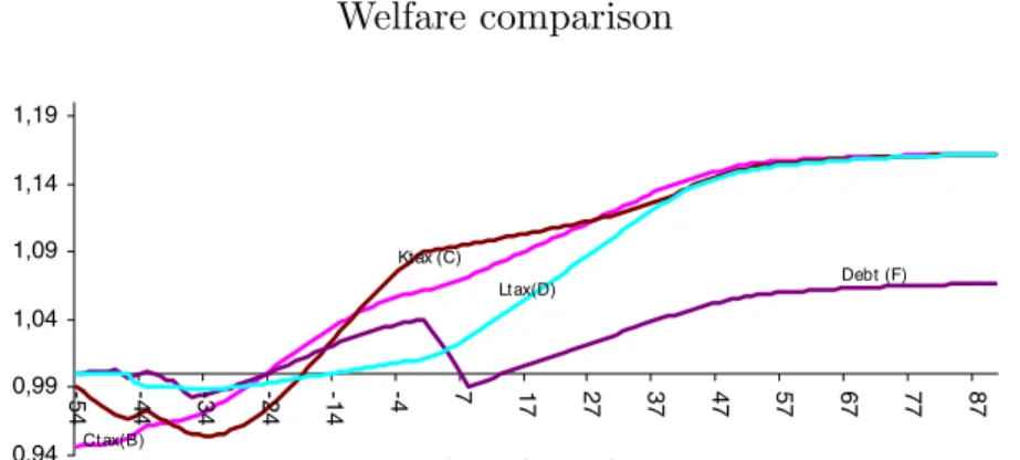
Figure 5 Welfare comparison
0,94 0,99 1,04 1,09 1,14 1,19
-5
4 -44 -34 -24 -14 -4 7 17 27 37 47 57 67 77 87
Ctax(B)
Ltax(D) Debt (F) Kt ax (C)
* Utility Ratio (Reform/Initial Steady State) over the Remaning Life
The consumption tax policy put most of the tax burden over the individuals “born” before year T = −25.33 The capital tax scheme focuses on middle aged workers and is the least preferred option for individuals “born” between T = −40 and T = −18. Curiously, it is the most preferable among the extremely young (“born” betweenT =−9 andT = 1), because it leads to a fast recovery after some initial depression on income. The labor tax policy is the most equitable scheme, and imposes a relatively higher tax burden on the initial youth. Individuals “born” after T = −18 have less welfare gains under such a tax scheme. The debt-financing scheme redistributes the lifetime income from the unborn generations to the old and middle aged individuals in T = 1, with a permanently lower welfare impact in the long run.
Note that no tax path is strictly preferred by any of the generations alive by the time of the reform. In particular, the status quo is preferred by individuals born between years T = −42 and T = −26. Under this simple model is possible to potentially explain substantial resistance to switching to a private scheme. The
32
One measure of these utility differences is the equivalent percentage increase in full lifetime resources (assets plus the present value of earnings based on working full time) needed in the original PAYG regime to produce each cohort’s realized level of utility under the specified alter-native regime. Here, I will use the concept of rest of life (ROL) wealth equivalent, instead of lifetime wealth equivalent. The reason for doing so is that agents too old experience almost no losses in their lifetime utility, since the weight of their last years is small in their total life. So, I prefer to look at the ratio between their ROL utility when living x years under the transition scheme and their ROL utility if they had lived the same x years under the old PAYG regime. Such criterion makes the welfare impact independent on the number of years being considered.
33
reform financed by labor tax leads to smaller intergenerational redistribution, but it is not the most preferred by any of the individuals alive, since it leads to slow convergence.
7.
Summary of the Experiments
The final welfare impact of each reform over the alive and the future gener-ations will be a result both of the direct impact of the tax instruments on their lifetime income and of the indirect impact, through general equilibrium effects of the reforms. The main conclusions from the simulations are summarized below:
First, the convergence is faster if the tax policy shifts more lifetime resources from the initial old to the initial youths, as it is the case under cold turkey, consumption tax transition and capital tax transition. The intuition is simple: old individuals are dis-saving and do not work. Shifting lifetime resources from this group will rapidly reduce aggregate consumption and will increase aggregate labor supply.
Secondly, consumption tax schemes lead to substantial welfare losses to the initial older generation, but higher lifetime wealth for those born in the ten years following the tax switch, even when there is no elimination of retirement benefits. Even when the PAYG remains unchanged and there is only a switch from labor tax to consumption tax in the financing of retirement benefits, the welfare gain of the individuals in T=10 are just slightly smaller than the gains obtained by the same individuals if benefits were reduced to zero. Such welfare improvement is driven by the fast convergence.
Third, increasing capital tax can lead to substantially negative impacts on the domestic capital, especially if benefits are not eliminated, as it is the case in experiment L. Such tax scheme transfers lifetime resources from high savers middle aged to prodigal youths, hurting especially the initial middle-aged individuals.
Postponing the tax adjustment, by accumulating government debt, mostly benefits the middle aged and elderly, and raises the long run tax rate. Hence, it is a redistribution from all future generations to the alive ones.
Delaying the elimination of the social security tax transfers lifetime resources from the current youths and individuals born in the first 25 years of the transition to the elderly and middle aged, and (in cases H and I) to the individuals born after year T = 50. The group of “losers” will not enjoy the large tax relieve coming from the elimination of the social security tax. The elderly will not suffer any elimination of retirement benefits. The individuals born after T = 50 will enjoy even greater tax reduction, since the accumulation of a surplus reduces the stock of government debt.
Fifth, special attention is devoted to the demand for foreign capital during the transition. Fully privatizing the system generates substantial reductions in the stock of foreign liability in the long run, but the short run results are completely different and may determine the interruption of the transition if the country faces a temporary borrowing constraint. The most obvious example is when capital tax finances the remaining retirement benefits. Experiment C shows that under such tax scheme the current account deficit would reach 5% of GNP on average in the first ten years. Financing this demand for foreign capital would require the stock of foreign liability to reach 200% of GNP in the first twenty years.
On the other hand, a consumption tax scheme would render a fast transition. The demand for foreign capital would decrease substantially, and by the year
T = 25 the ratioKt∗/GN Pt would reach 120%, compared to 186% under a capital
tax. It is clear that a capital tax transition might make the economy more subject to some sort of financial instability during the first years of the transition. Alter-natively, increasing the government debt during the transition and postponing the tax adjustment would keep the foreign liability above the initial steady state level for nearly 50 years. Hence, the same conclusions for the capital tax apply in this case.
100% to 30% are about 75% of the total welfare gain of full privatization (experi-ment J). Such a result argues strongly in favor of some sort of mixed system, with a minimum retirement income financed by a small tax on labor.
8.
Conclusions
This paper differs from Ferreira (2002) and Kotlikoff (1996) on the assump-tion of free capital mobility, which leads to an exogenous and (assumed) constant interest rate. Because the production function presents constant returns to scale, this implies that the marginal productivity of capital is homogeneous of degree zero, and leads to a constant capital-labor ratio. Hence the marginal productivity of labor is constant as well.
Taking as the example the case where the PAYG is eliminated, in Ferreira (2002) the variation in the relative factor prices lessens the impact of social security reforms on capital accumulation. Under an open economy, there will be a much larger impact on the domestic capital accumulation (since the interest rate does not fall as a result of higher savings). Under the closed economy, the marginal productivity of labor increases and hence there is an increase in aggregate labor supply in the long run.
Under the open economy case, the effect of changes in the relative price of labor (resulting from the tax elimination) is more than offset by income effects resulting from higher capital income, and there is a slight fall in aggregate labor supply. The aggregate total capital (which is equal to the capital owned by residents in the closed economy case) will follow the same path of the aggregate labor supply, since wage and interest rate are constant over the transition.
Incorporating features of an open economy in this paper allows one to think about impact on the current account of reforms of large magnitude. Results in this paper shows that financing the transition to a fully funded system will lead to completely different impacts on the current account, depending on the tax chosen.
References
Altig, D., Auerbach, A. J., Kotlikoff, L. J., Smetters, K. A., & Walliser, J. (2001). Simulating fundamental tax reform in the United States. American Economic Review, 91(3):574–95.
transfers: Theory and evidence. Journal of Political Economy, 105(6):1121– 1166.
Auerbach, A. & Kotlikoff, L. (1987).Dynamic Fiscal Policy. Cambridge University Press, Cambridge.
Barreto, F. & Oliveira, L. (2000). Transi¸c˜ao para regimes previdenci´arios de cap-italiza¸c˜ao e seus efeitos macroeconˆomicos de longo prazo no Brasil. Estudos Econˆomicos, 31(1):57–87.
Boldrin, M. & Rustichini, A. (1998). Political equilibria with social security. Re-view of Economic Dynamics, 3:41–78.
Bugarin, M., Ellery Jr., R., Gomes, V., & Teixeira, A. (2002). The Brazilian depression in the 1980s and 1990s. Unpublished manuscript, 2002.
Cooley, T. & Soares, J. (1999). A positive theory of social security based on reputation. Journal of Political Economy, 107(1):135–160.
De Nardi, M., Imrohoroglu, S., & Sargent, T. (1999). Projected US demographics and social security. Review of Economic Dynamics, 2(3):575–615.
Deaton, A., Gourinchas, P., & Paxson, C. (2002). Social security and inequality over the life cycle. In Feldstein, M. & Liebman, J. (eds.), editor, The Distri-butional Aspects of Social Security and Social Security Reform. University of Chicago Press, Chicago. NBER Conference report Series.
Ferreira, S. (2002). Macroeconomic and welfare effects of social security reforms. proceedings of the North American meeting of the econometric society. Summer. Los Angeles.
Ghez, G. & Becker, G. (1975). The Allocation of Time and Goods over the Life Cycle. Columbia University Press, New York.
Imrohoroglu, A., Imrohoglu, S., & Joines, D. (2002). Time inconsistency prefer-ences and social security. Proceedings of the North American Meeting of the Econometric Society, Summer. Los Angeles.
Issler, J. & Piqueira, N. (2000). Estimating relative risk aversion, the discount rate, and the intertemporal elasticity of substitution in consumption for Brazil using three types of utility function.Brazilian Review of Econometrics, 20(2):201–239.
Kotlikoff, L. (1996). Simulating the privatization of social security in general equilibrium. In Feldstein, M., editor, Privatizing Social Security – Chicago and London, pages 265–306. University of Chicago Press.
Kotlikoff, L., Smetters, K., & Walliser, J. (1998a). Opting out of social security and adverse selection. NBER Working Paper: 6430.
Kotlikoff, L., Smetters, K., & Walliser, J. (1998b). Social security: Privatization and progressivity. American Economic Review, 88(2):137–141.
McGarry, K. & Schoeni, R. (1995). Transfer behavior: Measurement and the redistribution of resources within the family. Journal of Human Resources, 30(5):S184–S226.
Appendix A
Table A.1
Individual labor supply – year 1
Cohort (T = 1) 21 30 40 50 55 60 65 70 75
Experiments Steady State 76,16 77,35 74,91 67,06 59,78 48,74 39,95 5,52 0 A Cold Turkey 76,35 77,85 76,3 70,62 65,67 59,24 53,03 37,09 10,33 B Consumption 76,13 77,62 75,88 69,36 63,1 53,35 38,31 15,24 0 C Capital 75,4 77,52 76,46 70,53 64,43 54,69 39,74 17,21 0 D Labor 75,82 77,17 74,91 67,3 60,16 49,23 32,41 5,34 0 E Income 75,8 77,45 75,71 68,9 62,26 51,9 35,95 11,12 0 F Debt - 7 77,58 78,93 77,14 70,67 64,50 54,43 39,20 15,77 0 G Antec. 20 yrs 75,82 77,27 75,25 67,94 60,33 49,08 40,30 6,45 0 H Antec. 20 yrs 75,76 77,21 75,15 67,77 60,07 48,70 39,91 5,55 0 I Antec. 20 yrs 75,77 77,22 75,17 67,78 60,07 48,70 39,91 5,55 0 J R=30% 75,87 77,19 74,94 67,41 60,38 49,68 40,94 6,99 0 K R=100%, C.tax 76,21 77,65 75,83 69,17 62,85 53,19 38,31 15,25 0 L R=100%, I. tax 75,95 77,50 75,63 68,63 61,94 51,70 35,94 11,14 0
Table A.2
Individual consumption - year 1
Table A.3
Transition - domestic capital
Year 1 5 10 19 25 50 75 100 150
A Cold Turkey 100 110 121 135 141 152 154 155 155 B Consumption 100 103 107 115 120 135 148 154 155 C Capital 100 97 95 95 98 125 147 153 155 D Labor 100 100 101 103 106 123 145 153 155 E Income 100 99 99 101 104 126 146 153 155 F Debt - 7 100 100 98 96 96 98 109 114 15 G Antec. 20 yrs 100 101 102 105 110 137 152 154 155 H Antec. 20 yrs 100 101 102 103 109 137 154 156 157 I Antec. 20 yrs 100 101 102 104 109 142 161 164 165 J R=30% 100 101 102 105 107 119 132 138 140 K R=100%, C.tax 100 103 106 112 115 120 121 122 122 L R=100%, I.tax 100 99 98 96 95 93 91 90 89
Table A.4
Transition - labor supply and total capital stock
Year 1 5 10 19 25 50 75 100 150
Table A.5
Transition - consumption
Year 1 5 10 19 25 50 75 100 150
A Cold Turkey 99,8 103,3 108,1 114,9 117,7 123,2 124,3 124,5 124,5 B Consumption 100,2 101,2 102,5 105,8 108,0 115,7 121,2 123,9 124,5 C Capital 106,4 105,2 103,8 102,0 102,2 111,2 120,3 123,7 124,5 D Labor 99,5 99,6 99,9 101,4 102,7 110,9 119,5 123,6 124,5 E Income 102,5 102,0 101,6 102,1 103,1 111,3 119,9 123,7 124,5 F Debt - 7 104,7 105,1 99,8 99,5 99,6 101,2 105,0 107,4 108,1 G Antec. 20 yrs 100,4 100,5 100,9 102,0 106,7 115,6 123,1 124,2 124,5 H Antec. 20 yrs 99,6 99,7 100,0 101,0 105,8 115,6 123,8 124,9 125,3 I Antec. 20 yrs 99,6 99,7 99,9 100,9 106,2 117,2 126,8 128,2 128,6 J R=30% 100,5 100,8 101,4 102,7 103,8 108,7 114,0 117,0 118,0 K R=100%, C.tax 100,4 101,4 102,6 104,7 106,0 108,9 109,4 109,6 109,6 L R=100%, I. tax 102,7 102,2 101,7 101,0 100,6 99,3 98,6 98,2 97,7 Obs: YearT = 0 = 100
Table A.6 Transition - income
Year 1 5 10 19 25 50 75 100 150
Table A.7
Transition - net foreign liability (%GNP)
Year 1 5 10 19 25 50 75 100 150
A Cold Turkey 187% 158% 126% 89% 73% 46% 42% 41% 40% B Consumption 173% 164% 152% 132% 120% 86% 55% 43% 40% C Capital 176% 185% 194% 196% 186% 112% 59% 44% 40% D Labor 164% 164% 162% 159% 155% 118% 62% 44% 40% E Income 170% 172% 174% 170% 163% 111% 61% 44% 40% F Debt - 7 178% 179% 166% 176% 178% 177% 146% 132% 128% G Antec. 20 yrs 166% 164% 159% 151% 155% 83% 47% 42% 40% H Antec. 20 yrs 166% 163% 160% 154% 158% 83% 44% 38% 37% I Antec. 20 yrs 166% 163% 160% 152% 158% 75% 29% 23% 22% J R=30% 166% 165% 162% 156% 151% 122% 91% 75% 70% K R=100%, C.tax 173% 165% 155% 139% 131% 115% 112% 111% 110% L R=100%, I. tax 170% 173% 177% 182% 184% 191% 197% 200% 203% Obs: YearT = 0 = 165%.
Table A.8
Transition - domestic savings
Year 0 1 5 10 25 50 75 100 150
Table A.9
Transition - current account
Year 0 1 5 10 25 50 75 100 150
A Cold Turkey -3,14% 2,67% 2,99% 2,79% 0,64% -0,54% -0,72% -0,76% -0,77% B Consumption -3,14% -1,32% -1,05% -1,01% -0,71% -0,48% -0,19% -0,66% -0,77% C Capital -3,14% -5,45% -5,32% -4,85% -1,74% 0,44% -0,05% -0,63% -0,77% D Labor -3,14% -3,07% -2,93% -3,33% -2,35% -0,02% 0,15% -0,62% -0,77% E Income -3,14% -3,83% -3,61% -3,61% -1,99% 0,10% 0,05% -0,62% -0,77% F Debt - 7 -3,14% -3,29% -3,73% -4,59% -3,56% -2,97% -1,90% -2,31% -2,43% G Antec. 20 yrs -3,14% -2,61% -2,40% -2,17% -0,32% 0,74% -0,58% -0,70% -0,77% H Antec. 20 yrs -3,14% -2,75% -2,55% -2,34% -0,26% 0,95% -0,49% -0,63% -0,70% I Antec. 20 yrs -3,14% -2,73% -2,52% -2,26% 0,08% 1,41% -0,14% -0,33% -0,41% J R=30% -3,14% -3,12% -2,89% -2,68% -2,14% -1,24% -0,80% -1,17% -1,33% K R=100%, C.tax -3,14% -1,50% -1,35% -1,28% -1,37% -2,00% -2,07% -2,09% -2,10% L R=100%, I. tax -3,14% -4,04% -3,96% -3,88% -3,80% -3,88% -3,88% -3,87% -3,87%
Table A.10
Rest of life utility - wealth equivalent
Cohort (T = 1) 21 30 40 50 55 60 65 70 75 A Cold Turkey 14% 13% 9% 3% -2% -8% -21% -24% -23% B Consumption 6% 5% 2% -1% -3% -4% -4% -5% -5% C Capital 9% 5% 0% -4% -5% -4% -3% -3% -1%
D Labor 1% 0% 0% -1% -1% -1% -1% 0% 0%
E Income 5% 3% 0% -2% -2% -2% -2% -1% 0% F Debt - 7 4% 3% 1% -1% -2% -1% 0% 0% 0% G Antec. 20 yrs 2% 1% 0% -2% 0% 0% 0% 0% 0% H Antec. 20 yrs 2% 1% -1% -2% -1% 0% 0% 0% 0% I Antec. 20 yrs 2% 1% -1% -2% -1% 0% 0% 0% 0%
J R=30% 2% 2% 1% 0% -1% -1% -1% -1% 0%
Table A.11
Lifetime utility - wealth equivalent
“Birth” Year 1 5 10 25 50 75 100 150
Appendix B
Table B.1
Instantaneous elimination of benefits - experiment A
Year Kd K C GNP Average Tax Rates Sn CA K* Welfare Age Welfare
(1) (2) (3) (4) (5) C K L (6) (7) (8) (9) (10) (11)
Initial st.st. 100 100 100 100 15,0% 13,0% 30,4% 4,00% -3,14% 165% 0% 75 -23% 1 100 108 100 105 15,0% 12,4% 18,2% 8,42% 2,67% 187% 14% 70 -24% 5 110 107 103 108 14,5% 12,1% 18,0% 8,34% 2,99% 158% 15% 60 -8% 10 121 105 108 111 13,9% 11,8% 17,7% 7,75% 2,79% 126% 15% 50 3% 25 141 102 118 116 12,7% 11,3% 17,5% 6,07% 0,64% 73% 16% 45 6% 50 152 100 123 119 12,2% 11,0% 17,3% 5,07% -0,54% 46% 16% 40 9% 75 154 100 124 119 12,1% 11,0% 17,3% 4,90% -0,72% 42% 16% 30 13% Final st.st. 155 100 125 119 12,0% 11,0% 17,3% 4,85% -0,77% 40% 16% 25 14% Column (1) - year of transition; Column (2) - Domestic Capital; Column (3) - Total Capital ; Column (4) - Consumption; Column (5) - National Income;
Columns (2) to (5) - Index initial steady state = 100;
Column (3) is the aggregate labor as well, since K and L are proportional;
Column (6) - Net National saving rate; Column (7) - Current Account Surplus ((-) is a deficit); Column (8) - Foreign Capital or Net Foreign Liability; Columns (6) to (8) in % GNP;
Column (9) - Wealth Equivalent of a person born in that year, with respect to wealth equivalent of person born during steady state. Column (10) - Actual age of the person in yearT = 1; Column (11) - ROL Utility (Measured by Wealth Equivalent) of a person with that age in T = 1, compared to the situation when no policy change is implemented.
Table B.2
Consumption tax - experiment B
Year Kd K C GNP Average Tax Rates Sn CA K* Welfare Age Welfare
(1) (2) (3) (4) (5) C K L (6) (7) (8) (9) (10) (11)
Initial st.st. 100 100 100 100 15,0% 13,0% 30,4% 4,00% -3,14% 165% 0% 75 -5% 1 100 103 100 102 23,7% 13,0% 20,0% 5,56% -1,32% 173% 6% 70 -5% 5 103 103 101 103 23,5% 13,0% 20,0% 5,69% -1,05% 164% 7% 60 -4% 10 107 102 103 104 22,9% 13,0% 20,0% 5,86% -1,01% 152% 8% 50 -1% 25 120 102 108 108 18,0% 13,0% 20,0% 5,87% -0,71% 120% 11% 45 0% 50 135 102 116 114 13,3% 11,8% 18,1% 5,56% -0,48% 86% 15% 40 2% 75 148 101 121 118 12,4% 11,1% 17,4% 5,40% -0,19% 55% 16% 30 5% Final st.st. 155 100 125 119 12,0% 11,0% 17,3% 4,85% -0,77% 40% 16% 25 6% Column (1) - year of transition; Column (2) - Domestic Capital; Column (3) - Total Capital ; Column (4) - Consumption; Column (5) - National Income;
Columns (2) to (5) - Index initial steady state = 100;
Column (3) is the aggregate labor as well, since K and L are proportional;
Column (6) - Net National saving rate; Column (7) - Current Account Surplus ((-) is a deficit); Column (8) - Foreign Capital or Net Foreign Liability; Columns (6) to (8) in % GNP;
Table B.3
Capital tax - experiment C
Year Kd K C GNP Average Tax Rates Sn CA K* Welfare Age Welfare
(1) (2) (3) (4) (5) C K L (6) (7) (8) (9) (10) (11)
Initial st.st. 100 100 100 100 15,0% 13,0% 30,4% 4,00% -3,14% 165% 0% 75 -1% 1 100 104 106 103 15,0% 26,3% 20,0% 2,31% -5,45% 176% 9% 70 -3% 5 97 105 105 102 15,0% 27,5% 20,0% 2,48% -5,32% 185% 9% 60 -4% 10 95 105 104 102 15,0% 28,6% 20,0% 3,00% -4,85% 194% 10% 50 -4% 25 98 106 102 103 15,0% 22,6% 20,0% 5,32% -1,74% 186% 11% 45 -2% 50 125 104 111 112 13,8% 12,0% 18,3% 6,38% 0,44% 112% 15% 40 0% 75 147 101 120 117 12,5% 11,2% 17,4% 5,53% -0,05% 59% 16% 30 5% Final st.st. 155 100 125 119 12,0% 11,0% 17,3% 4,85% -0,77% 40% 16% 25 8% Column (1) - year of transition; Column (2) - Domestic Capital; Column (3) - Total Capital ; Column (4) - Consumption; Column (5) - National Income;
Columns (2) to (5) - Index initial steady state = 100;
Column (3) is the aggregate labor as well, since K and L are proportional;
Column (6) - Net National saving rate; Column (7) - Current Account Surplus ((-) is a deficit); Column (8) - Foreign Capital or Net Foreign Liability; Columns (6) to (8) in % GNP;
Column (9) - Wealth Equivalent of a person born in that year, with respect to wealth equivalent of person born during steady state. Column (10) - Actual age of the person in yearT = 1; Column (11) - ROL Utility (Measured by Wealth Equivalent) of a person with that age in T = 1, compared to the situation when no policy change is implemented.
Table B.4
Labor tax - experiment D
Year Kd K C GNP Average Tax Rates Sn CA K* Welfare Age Welfare
(1) (2) (3) (4) (5) C K L (6) (7) (8) (9) (10) (11)
Initial st.st. 100 100 100 100 15,0% 13,0% 30,4% 4,00% -3,14% 165% 0% 75 0% 1 100 100 99 100 15,0% 13,0% 30,5% 4,18% -3,07% 164% 1% 70 0% 5 100 100 100 100 15,0% 13,0% 30,3% 4,27% -2,93% 164% 2% 60 -1% 10 101 100 100 100 15,0% 13,0% 29,7% 4,41% -3,33% 162% 3% 50 -1% 25 106 102 103 103 15,0% 13,0% 25,4% 5,04% -2,35% 155% 8% 45 -1% 50 123 104 111 111 13,9% 12,1% 18,3% 6,11% -0,02% 118% 15% 40 0% 75 145 101 119 117 12,6% 11,2% 17,4% 5,71% 0,15% 62% 16% 30 0% Final st.st. 155 100 125 119 12,0% 11,0% 17,3% 4,85% -0,77% 40% 16% 25 1% Column (1) - year of transition; Column (2) - Domestic Capital; Column (3) - Total Capital ; Column (4) - Consumption; Column (5) - National Income;
Columns (2) to (5) - Index initial steady state = 100;
Column (3) is the aggregate labor as well, since K and L are proportional;
Column (6) - Net National saving rate; Column (7) - Current Account Surplus ((-) is a deficit); Column (8) - Foreign Capital or Net Foreign Liability; Columns (6) to (8) in % GNP;
Table B.5
Income tax - experiment E
Year Kd K C GNP Average Tax Rates Sn CA K* Welfare Age Welfare
(1) (2) (3) (4) (5) C K L (6) (7) (8) (9) (10) (11)
Initial st.st. 100 100 100 100 15,0% 13,0% 30,4% 4,00% -3,14% 165% 0% 75 0% 1 100 102 102 101 15,0% 18,8% 25,8% 3,53% -3,83% 170% 5% 70 -1% 5 99 102 102 101 15,0% 18,8% 25,8% 3,71% -3,61% 172% 5% 60 -2% 10 99 102 102 101 15,0% 18,8% 25,8% 4,02% -3,61% 174% 6% 50 -2% 25 104 104 103 104 15,0% 16,2% 23,2% 5,22% -1,99% 163% 9% 45 -1% 50 126 103 111 111 13,8% 12,1% 18,3% 6,14% 0,10% 111% 15% 40 0% 75 146 101 120 117 12,5% 11,2% 17,4% 5,62% 0,05% 61% 16% 30 3% Final st.st. 155 100 125 119 12,0% 11,0% 17,3% 4,85% -0,77% 40% 16% 25 4% Column (1) - year of transition; Column (2) - Domestic Capital; Column (3) - Total Capital ; Column (4) - Consumption; Column (5) - National Income;
Columns (2) to (5) - Index initial steady state = 100;
Column (3) is the aggregate labor as well, since K and L are proportional;
Column (6) - Net National saving rate; Column (7) - Current Account Surplus ((-) is a deficit); Column (8) - Foreign Capital or Net Foreign Liability; Columns (6) to (8) in % GNP;
Column (9) - Wealth Equivalent of a person born in that year, with respect to wealth equivalent of person born during steady state. Column (10) - Actual age of the person in yearT = 1; Column (11) - ROL Utility (Measured by Wealth Equivalent) of a person with that age in T = 1, compared to the situation when no policy change is implemented.
Table B.6
Year fiscal deficit - experiment F
Year Kd K C GNP Average Tax Rates Sn CA K* Welfare Age Welfare
(1) (2) (3) (4) (5) C K L (6) (7) (8) (9) (10) (11)
Initial st.st. 100 100 100 100 15,0% 13,0% 30,4% 4,00% -3,14% 165% 30% 0% 75 0% 1 100 105 105 103 15,0% 13,0% 20,0% 3,80% -3,29% 178% 29% 4% 70 0% 5 100 105 105 103 15,0% 13,0% 20,0% 3,39% -3,73% 179% 50% 1% 60 -1% 10 98 98 100 98 22,2% 18,1% 27,5% 2,66% -4,59% 166% 78% -1% 50 -1% 25 96 100 100 99 20,9% 16,9% 25,6% 3,24% -3,56% 178% 78% 2% 45 0% 50 98 103 101 101 18,8% 15,2% 23,0% 4,04% -2,97% 177% 76% 6% 40 1% 75 109 102 105 104 17,8% 14,5% 22,2% 4,40% -1,90% 146% 74% 6% 30 3% Final st.st. 115 101 108 106 17,2% 14,3% 22,0% 3,89% -2,43% 128% 72% 7% 25 4% Column (1) - year of transition; Column (2) - Domestic Capital; Column (3) - Total Capital ; Column (4) - Consumption; Column (5) - National Income;
Columns (2) to (5) - Index initial steady state = 100;
Column (3) is the aggregate labor as well, since K and L are proportional;
Column (6) - Net National saving rate; Column (7) - Current Account Surplus ((-) is a deficit); Column (8) - Foreign Capital or Net Foreign Liability; Columns (6) to (8) in % GNP;
Table B.7
Experiment G - 20 yrs announcement - endogenous tax rate
Year Kd K C GNP Average Tax Rates Sn CA K* Welfare Age Welfare
(1) (2) (3) (4) (5) C K L (6) (7) (8) (9) (10) (11)
Initial st.st. 100 100 100 100 15,0% 13,0% 30,4% 4,00% -3,14% 165% 0% 75 0% 1 100 101 100 100 14,9% 13,0% 29,5% 4,07% -2,61% 166% 2% 70 0% 5 101 100 101 101 14,9% 12,9% 29,6% 4,20% -2,40% 164% 4% 60 0% 10 102 100 101 101 14,9% 12,9% 29,6% 4,31% -2,17% 159% 6% 50 -2% 25 110 106 107 107 14,1% 12,2% 18,1% 5,86% -0,32% 155% 14% 45 -2% 50 137 102 116 115 13,0% 11,4% 17,6% 6,30% 0,74% 83% 16% 40 0% 75 152 100 123 119 12,2% 11,0% 17,3% 5,04% -0,58% 47% 16% 30 1% Final st.st. 155 100 125 119 12,0% 11,0% 17,3% 4,85% -0,77% 40% 16% 25 2% Column (1) - year of transition; Column (2) - Domestic Capital; Column (3) - Total Capital ; Column (4) - Consumption; Column (5) - National Income;
Columns (2) to (5) - Index initial steady state = 100;
Column (3) is the aggregate labor as well, since K and L are proportional;
Column (6) - Net National saving rate; Column (7) - Current Account Surplus ((-) is a deficit); Column (8) - Foreign Capital or Net Foreign Liability; Columns (6) to (8) in % GNP;
Column (9) - Wealth Equivalent of a person born in that year, with respect to wealth equivalent of person born during steady state. Column (10) - Actual age of the person in yearT = 1; Column (11) - ROL Utility (Measured by Wealth Equivalent) of a person with that age in T = 1, compared to the situation when no policy change is implemented.
Table B.8
Experiment H - 20 yrs announcement - 20 yrs surplus
Year Kd K C GNP Average Tax Rates Sn CA K* Welfare Age Welfare
(1) (2) (3) (4) (5) C K L (6) (7) (8) (9) (10) (11)
Initial st.st. 100 100 100 100 15,0% 13,0% 30,4% 4,00% -3,14% 165% 30% 0% 75 0% 1 100 100 100 100 15,0% 13,0% 30,4% 4,34% -2,75% 166% 29% 2% 70 0% 5 101 100 100 100 15,0% 13,0% 30,4% 4,46% -2,55% 163% 29% 3% 60 0% 10 102 100 100 101 15,0% 13,0% 30,5% 4,55% -2,34% 160% 29% 5% 50 -2% 25 103 99 101 101 14,0% 12,1% 18,0% 5,98% -0,26% 158% 25% 15% 45 -2% 50 109 106 106 107 12,8% 11,3% 17,4% 6,47% 0,95% 83% 24% 16% 40 -1% 75 137 102 116 115 12,0% 10,9% 17,1% 5,11% -0,49% 44% 23% 17% 30 1% Final st.st. 156 100 125 120 11,8% 10,8% 17,1% 4,89% -0,70% 37% 23% 17% 25 1% Column (1) - year of transition; Column (2) - Domestic Capital; Column (3) - Total Capital ; Column (4) - Consumption; Column (5) - National Income;
Columns (2) to (5) - Index initial steady state = 100;
Column (3) is the aggregate labor as well, since K and L are proportional;
Column (6) - Net National saving rate; Column (7) - Current Account Surplus ((-) is a deficit); Column (8) - Foreign Capital or Net Foreign Liability; Columns (6) to (8) in % GNP;
Table B.9
Experiment I - 20 yr. announcement - 25 yr. surplus
Year Kd K C GNP Average Tax Rates Sn CA K* Welfare Age Welfare
(1) (2) (3) (4) (5) C K L (6) (7) (8) (9) (10) (11)
Initial st.st. 100 100 100 100 15,0% 13,0% 30,4% 4,00% -3,14% 165% 30% 0% 75 -100% 1 100 100 100 100 15,0% 13,0% 30,4% 4,36% -2,73% 166% 29% -98% 70 -100% 5 101 100 100 100 15,0% 13,0% 30,4% 4,50% -2,52% 163% 29% -97% 60 -100% 10 102 100 100 101 15,0% 13,0% 30,5% 4,63% -2,26% 160% 29% -95% 50 -102% 25 104 99 101 101 13,3% 11,6% 17,2% 6,25% 0,08% 158% 16% -84% 45 -2% 50 109 107 106 107 12,0% 10,7% 16,5% 6,83% 1,41% 75% 15% -82% 40 -101% 75 142 103 117 117 11,1% 10,3% 16,2% 5,34% -0,14% 29% 15% -81% 30 -99% Final st.st. 164 99 128 123 10,9% 10,2% 16,1% 5,06% -0,41% 22% 14% -81% 25 1% Column (1) - year of transition; Column (2) - Domestic Capital; Column (3) - Total Capital ;
Column (4) - Consumption; Column (5) - National Income; Columns (2) to (5) - Index initial steady state = 100;
Column (3) is the aggregate labor as well, since K and L are proportional;
Column (6) - Net National saving rate; Column (7) - Current Account Surplus ((-) is a deficit); Column (8) - Foreign Capital or Net Foreign Liability; Columns (6) to (8) in % GNP;
Column (9) - Wealth Equivalent of a person born in that year, with respect to wealth equivalent of person born during steady state. Column (10) - Actual age of the person in yearT = 1; Column (11) - ROL Utility (Measured by Wealth Equivalent) of a person with that age in T = 1, compared to the situation when no policy change is implemented.
Table B.10
Experiment J - replacement rate reduced to 30%
Year Kd K C GNP Average Tax Rates Sn CA K* Welfare Age Welfare
(1) (2) (3) (4) (5) C K L (6) (7) (8) (9) (10) (11)
Initial st.st. 100 100 100 100 15,0% 13,0% 30,4% 4,00% -3,14% 165% 0% 75 0% 1 100 100 101 100 14,9% 13,0% 29,6% 3,91% -3,12% 166% 2% 70 -1% 5 101 101 101 101 14,9% 12,9% 29,1% 4,05% -2,89% 165% 3% 60 -1% 10 102 101 101 101 14,8% 12,8% 28,4% 4,20% -2,68% 162% 4% 50 0% 25 105 101 103 103 14,5% 12,6% 26,2% 4,57% -2,14% 151% 6% 45 0% 50 107 102 104 103 13,8% 12,1% 22,6% 5,12% -1,24% 122% 10% 40 1% 75 119 102 109 108 13,2% 11,7% 21,0% 5,10% -0,80% 91% 12% 30 2% Final st.st. 138 100 117 114 12,7% 11,5% 20,8% 4,55% -1,33% 70% 12% 25 2% Column (1) - year of transition; Column (2) - Domestic Capital; Column (3) - Total Capital ; Column (4) - Consumption; Column (5) - National Income;
Columns (2) to (5) - Index initial steady state = 100;
Column (3) is the aggregate labor as well, since K and L are proportional;
Column (6) - Net National saving rate; Column (7) - Current Account Surplus ((-) is a deficit); Column (8) - Foreign Capital or Net Foreign Liability; Columns (6) to (8) in % GNP;
Table B.11
Experiment K - payroll tax switched off, replaced by consumption tax
Year Kd K C GNP Average Tax Rates Sn CA K* Welfare Age Welfare
(1) (2) (3) (4) (5) C K L (6) (7) (8) (9) (10) (11)
Initial st.st. 100 100 100 100 15,0% 13,0% 30,4% 4,00% -3,14% 165% 0% 75 -5% 1 100 103 100 102 23,7% 13,0% 20,0% 5,37% -1,50% 173% 6% 70 -5% 5 103 103 101 103 23,5% 13,0% 20,0% 5,40% -1,35% 165% 6% 60 -3% 10 106 102 103 104 23,1% 13,0% 20,0% 5,40% -1,28% 155% 6% 50 -1% 25 112 102 105 105 21,8% 13,0% 20,0% 5,20% -1,37% 131% 7% 45 1% 50 115 101 106 106 20,8% 13,0% 20,0% 4,63% -2,00% 115% 7% 40 2% 75 120 100 109 107 20,6% 13,0% 20,0% 4,55% -2,07% 112% 7% 30 4% Final st.st. 122 100 110 108 20,5% 13,0% 20,0% 4,52% -2,10% 110% 7% 25 5% Column (1) - year of transition; Column (2) - Domestic Capital; Column (3) - Total Capital ; Column (4) - Consumption; Column (5) - National Income;
Columns (2) to (5) - Index initial steady state = 100;
Column (3) is the aggregate labor as well, since K and L are proportional;
Column (6) - Net National saving rate; Column (7) - Current Account Surplus ((-) is a deficit); Column (8) - Foreign Capital or Net Foreign Liability; Columns (6) to (8) in % GNP;
Column (9) - Wealth Equivalent of a person born in that year, with respect to wealth equivalent of person born during steady state. Column (10) - Actual age of the person in yearT = 1; Column (11) - ROL Utility (Measured by Wealth Equivalent) of a person with that age in T = 1, compared to the situation when no policy change is implemented.
Table B.12
Experiment L - payroll tax switched off, replaced by income tax
Year Kd K C GNP Average Tax Rates Sn CA K* Welfare Age Welfare
(1) (2) (3) (4) (5) C K L (6) (7) (8) (9) (10) (11)
Year Kd K C GNP Average Tax Rates Sn CA K* Welfare Age Welfare
(1) (2) (3) (4) (5) C K L (6) (7) (8) (9) (10) (11)
Initial st.st. 100 100 100 100 15,0% 13,0% 30,4% 4,00% -3,14% 165% 0% 75 0% 1 100 102 103 101 15,0% 18,8% 25,8% 3,31% -4,04% 170% 4% 70 -1% 5 99 102 102 101 15,0% 18,9% 25,9% 3,37% -3,96% 173% 4% 60 -2% 10 98 102 102 101 15,0% 19,0% 26,0% 3,43% -3,88% 177% 3% 50 -1% 25 96 102 101 100 15,0% 19,3% 26,3% 3,55% -3,80% 184% 3% 45 -1% 50 95 102 101 100 15,0% 19,6% 26,6% 3,55% -3,88% 191% 3% 40 0% 75 93 102 99 99 15,0% 19,8% 26,8% 3,59% -3,88% 197% 3% 30 2% Final st.st. 90 103 98 98 15,0% 20,0% 27,0% 3,63% -3,87% 203% 2% 25 3% Column (1) - year of transition; Column (2) - Domestic Capital; Column (3) - Total Capital ; Column (4) - Consumption; Column (5) - National Income;
Columns (2) to (5) - Index initial steady state = 100;
Column (3) is the aggregate labor as well, since K and L are proportional;
Column (6) - Net National saving rate; Column (7) - Current Account Surplus ((-) is a deficit); Column (8) - Foreign Capital or Net Foreign Liability; Columns (6) to (8) in % GNP;
Appendix C
Table C.1
Parameterization of the initial steady state
Parametric Assumptions Policy Parameters
Proportional Consumption Tax: 15% Proportional Capital: 13%
Proportional Labor Tax: 20%
Social Security Links : 0, for age ¡ 43; 0.6, if age = 43; 0.8 if age = 44, and 1 if age = 45. D/K = 0.14
Real interest rate = 15% Preference Parameters: Intertemporal Discount Rate
Intertemporal elasticity of substitution (gamma): 0.305 Intratemporal elasticity of substitution (rho): 1.1 Leisure-preference parameter (alpha): 0.36 Technology Parameters:
wt,i=wtej =wtexp{−.2314 +.0529.j−.00093.j2}