Tiling in the Geometric Model for Water
M. Girardi, W. Figueiredo,
Departamento de F´ısica, Universidade Federal de Santa Catarina, 88040-900, Florian ´opolis, Santa Catarina, Brasil
N. Guisoni, and V. B. Henriques
Instituto de F´ısica, Universidade de S˜ao Paulo, C.P. 66318, CEP 05315-970, S˜ao Paulo, SP, Brasil
Received on 26 August, 2003.
Hydrogen bonded liquids like water present a rich thermodynamic behaviour due to the strength and direction-ality of the bonds. In a recent paper a geometric model based on Bernal’s model for liquids was proposed to study the effects of the hydrogen bonds on the phase transitions of water, under pressure and temperature vari-ations. Water molecules were assumed to stay at the vertices of coordinationr(r= 4,5,6) of perfectly tiled polygons, and to have four links which allow up to four hydrogen bonds per particle. Mean field calculations yielded a phase diagram with three phases of different densities and a critical point at the end of the coexistence line between the high and low density phases. The three phases were considered to be liquids of different den-sities. In the present work we have shown that applying some geometric constraints to particle arrangements (thus correcting the system entropy, which was overestimated in the previous work), and allowing a variable number of links per molecule, leads to substantial alteration of the phase diagram. Three phases of different densities are still present, but no critical point appears. Two of the phases are solid, and one phase is amorphous.
1
Introduction
Water and other hydrogen bonded liquids are known to exhibit many anomalous properties [1-10], which seem to arise from the strength and directionality of hydrogen bonds (HB), and ensuing low density. The HB network, which per-colates in liquid water, is thought to be responsible, among other things, for the increase of the isothermal compressibil-ity and constant pressure specific heat upon cooling, and for the isothermal compressibility minimum at46◦C.
In the context of molecular dynamics simulations, sev-eral microscopic models have been studied in an attempt to describe the peculiar properties of the associated liquid [1, 4, 5, 6]. These models focus attention mainly on the charge distribution on the rigid molecule and the parameters of the electrostatic and Lennard-Jones potential are adjusted to fit experimental data. Definition of hydrogen bonds de-pends on still controversial energetic and angular criteria, and are also parameter dependent.
A different approach is that of simplified models. In this case one hopes to include microscopic properties able to reproduce qualitatively the main features of liquid wa-ter behaviour, independently of adjustable paramewa-ters. One example is the square water model, which incorporates the directional character of the HB[10, 8, 11]. Square water is exactly solvable at T = 0 and gives an excellent es-timation of the residual entropy of the ice [12]. The HB number is a decreasing function of temperature, but the model does not present an order-disorder transition driven by temperature[10, 8, 11]. Under an external electric field, the system displays a structural phase transition[10] at T=0.
Used as a solvent, square water presents hydrophobic hydra-tion [8], albeit insufficient to explain water solubility prop-erties.
Density fluctuations seem to be an essential ingredi-ent. The geometric model for water, proposed by two of us [9], allows for changes in the local environment of the molecules. It is based on the geometric description of liq-uids given by Bernal [13], and developed on the plane by Collins[17] a few decades ago. In two dimensions, the wa-ter molecules are disposed at the vertices of squares and triangles of equal sides, perfectly tiling the plane. Such tiling yields coordination numbers for sites (vertex) given by r = 4,5 or 6. Four open links are allowed for each molecule, so that it can form up to four hydrogen bonds with itsrneighbors. A mean-field treatment of the model, adapted from a previous study[17] for the inclusion of HBs, yielded coexistence of three phases of different densities, and a critical point at the end of a high-low densities co-existence line. The three phases present no regularity, and therefore were interpreted as liquid phases.
To obtain the above results, a tiling constraint on entropy was left aside. It was assumed that the entropic term in the free energy has two contributions: one coming from the dis-tribution of four bonds amongrneighbors, and another one, coming from the number of geometric arrangements of the sites. Particles were treated as independent, therefore the geometric constraint of perfect tiling was not taken into ac-count in the calculation of the degeneracy of the spatial ar-rangements.
con-straint to the neighborhood of each site, in order to have a perfect tiling of squares and triangles at least at the nearest-neighboring sites. We have also allowed for a variable num-ber of links (nc = 2,3,4), in order to represent possible misalignment under temperature variations. The geomet-ric constraint on entropy was first calculated by Kawamura [14], for a purely hard core semi-infinite system and a solid-liquid transition was suggested. Similar corrections to en-tropy were found by Do et al. [15] and Yi et al. [16], in the treatment of the geometric model with a Lennard-Jones po-tential, for which they also proposed a melting line. We will show that the geometric correction for the water model pro-duces a substantial change of the phase diagram: two of the phases of different densities are crystalline and no critical point is present.
This article is organized as follows: in Sec. 2 we review the geometric model for water and introduce a variable num-ber of bonds per molecule. In Sec. 3 we perform a mean field calculation of the Gibbs free energy of the model, in which the constraint of tiling is introduced in the calculation of entropy. Finally, in Sec. 4, we present our discussions and conclusions.
2
The model
In 1960, Bernal proposed a geometric model for liquids, in which the fluid particles were placed at the vertices of reg-ular or quasi-regreg-ular polyhedra. The choice of these ran-domly distributed three-dimensional objects was motivated by the presence of local ordering, together with the absence of long range order in the liquid phase. Collins [17] con-sidered a two-dimensional version of Bernal’s model that consists of a perfect tiling of triangles and squares of equal sides. He found a discontinuous phase change for a special energy condition, from a mean-field calculation, which he suggested to be analogous to a change of association num-ber from one liquid phase to another. The noninteracting version of the model was employed later in the study of quasi-crystals [18, 19, 20], observed in alloy systems such as V-Ni and V-Ni-Si, in an attempt to explain their mecha-nism of formation.
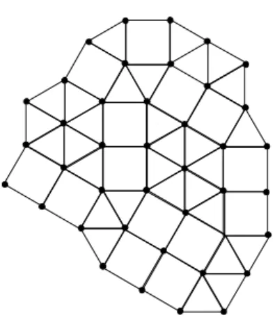
In Fig. 1, we show a typical configuration of the system in an amorphous phase. The ordered (crystalline) phases are the square and triangular lattices, where the plane is com-pletely filled by triangles or squares. The possible local structures around each site are shown in fig. 2. The sites can have three different coordination numbers1 (r = 4,5
and6), whose specific volumesvrare
v4=b2, (1)
v5=b2(2 +√3)/4, (2)
v6=b2√3/2, (3)
wherebis the intermolecular distance (polygon side), which is kept fixed (b = 1in this work). Each lattice site is occu-pied by a molecule, and we defineNras being the number of molecules withrneighbors. Volume and particle number
conservation give
X
r=4,5,6
Nr=N , (4)
X
r=4,5,6
Nrvr=V , (5)
whereV is the total volume and N is the total number of particles.
Figure 1. Typical configuration of the geometrical model for liq-uids (or a random square-triangle tiling) with intermediate density.
Hydrogen bonds will be defined as follows. Each molecule is connected to itsrneighbors byrlines. It may havenc = 2,3or4open links with itsrneighbors. These links may or may not be available due to, for example, orien-tational restraints and, if available, are distributed randomly over therlines. An HB will be present if two neighboring molecules point one of their links towards each other. In this way, the maximum number of hydrogen bonds for a given molecule isnc. In Fig. 2, (S1) and (S2) represent pairs of molecules at sites of the type A and B, with coordination numbers r = 4 and s = 5, respectively. In the case of (S1), the A molecule hasnc = 4links (represented by the full lines), and the B molecule, hasnc = 2. Only in (S2), where two links are in the line joining A and B, do we have a hydrogen bond between the two molecules.
Only hydrogen-bond energies shall be considered, since van der Waals interactions are one order of magnitude smaller than the hydrogen bond ones.
1
A B C D
S1 S2
Figure 2. The four possible configurations of the vertices: (A) ver-tex with coordination numberr = 4, (B) and (C) vertices with
r = 5but different geometries, and (D) vertex withr = 6. (S1) and (S2) represent two neighboring molecules and their links (full lines). In (S1) the upper molecule has four links, while the lower one has only two. There is not an HB between them. In (S2) there is one HB since two links are aligned.
3
Mean field calculations
In this section, we consider a mean field approximation in order to find the Gibbs free energy of the present geomet-ric model. The first step is to obtain the total energy of the system, which results solely from HBs. Following the defi-nition of the previous section (see Fig. 2), we may write, for the probability of an HB between two molecules (assuming they are independent) whose sites have coordination num-bersrands
PHB=n
r cnsc rs ≈
nc2
rs , (6)
wherenr
c(nsc) is the number of open links of a molecule with coordination numberr(s), andncis the fraction of links per
particle, which is independent of site-coordination. A natu-ral choice for the potential energy between two sites is then φrs =−εPHB(here,ε= 1).
The energy per particle is written as e{Ni}=X
rs
Crsφrs , (7)
where Crs is the number of (rs) nearest pairs, given by Crs= [rNrps(r)+sNspr(s)(1−δr,s)]. The functionps(r)
is the probability of a pair of neighboring sites with coordi-nation numbersrands, which is given by
ps(r) = Ns
Ntot(r) , (8)
where
Ntot(4) =N4+N5B+N5C , (9)
Ntot(5) =N , (10)
Ntot(6) =N5B+N5C+N6. (11) Here,N5BandN5C are the number of vertices of the type B andC, respectively (fig. 2). Ntot(r)is the number of neighbors to r particles, and the first neighbor geometric constraint, which precludes 4 and 6-particles from being neighbors is taken into account.
Now we must write the entropy of the system. Assum-ingN independent sites distributed among{Nr}sites, the number of spatial arrangements is simply
Ωo= N!
N4!N5B!N5C!N6!. (12)
The last expression overestimates the number of possible states of the system, since tiling constraints were not taken into account. To correct the number of states given by eq. 12, we consider the factor[14, 16]
⌋
F(N4, N5B, N5C, N6) = (n5B+n5C)N5B+2N5C (13) (n4+n5B)2N4+N5B/2(n4+n5B+n5C)N4+(N5B+N5C)/2
(n5B+n5C+n6)N5B+N5C/2+3N6 ,
⌈
wherenr = Nr/N. The correcting factor F guarantees a perfect arrangement of polygons at least for the nearest-neighboring sites. For a further explanation concerning this factor, see references 14 and 16. In this way, the number of states due to this geometric constraint becomes
Ωg(N4, N5B, N5C, N6) = ΩoF(N4, N5B, N5C, N6). (14) The newly calculated geometrically constrained number of spatial arrangements is significantly improved with re-spect to the non-constrained case. This can be seen from
comparison with the known entropy of the athermal ver-sion of the square-triangle tiling model, given the area frac-tion occupied by each component. The exact partifrac-tion func-tion for the latter was obtained using the Bethe ansatz and, for the case of equal area fractions, the entropy per vertex [19, 21, 22] is
sex= ln(2233)−2√3 ln(2 +√3)≃0.120.
sg ≃ 0.55, withs = kB
N ln Ω, indicating a significant im-provement of the estimated entropy by taking into account the constraint factorF.
We must yet compute the entropic contribution due to the distribution of the molecular links. Let us defineMncas
the number of sites withnclinks. Note thatMncsatisfies the
relationsM2+M3+M4=Nand2M2+3M3+4M4=Nc, whereNc = N nc. For a given set of values ofMnc, the
number of arrangements of sites havingnclinks is
Ωd=
N!
M2!M3!M4! . (15)
The number of states for a given site withr neighbors and nc links is the number of combinations of r over nc and, therefore, the total number of states accessible to the system is
Ω = ΩgΩd Y
r,nc
· r!
nc!(r−nc)!
¸Nr,nc
, (16)
whereNr,ncis the number of sites havingrneighbors and
nclinks, which in this mean field approximation we take as Nr,nc = NrMnc/N. The entropy per particle is given by
s=kB
N ln Ωand the partition function of the model is given by:
Z(T, P) = X′
{Ni, Mj} exp
·
−βN(e+P v−ln Ω
N β) ¸
, (17)
where P is the pressure, β = (kBT)−1, T is the tem-perature, and the prime in the summation indicates the constraints P
iNi = N and P
iMi = N. Writing ζ({Ni, Mj}) =e−T s+P v, we can identify the Gibbs free energy per particle as g(T, P) = ζ(T, P,{Ni, Mj}min), where {Ni, Mj}min is the set of values of Ni and Mj which minimizesζ. Solutions were sought for in the ranges
0 ≤Ni/N ≤1,0 ≤Mi/N ≤1and2 ≤nc¯ ≤4through thesimulated annealing[23] algorithm.
4
Results and conclusions
In Fig. 3 we exhibit the phase diagram of the model in the planeP versusT for both fixed (four) and variable number of links. As can be seen in the figure, the diagram presents three phases of different densities, a triple point (tp), and no critical point. Note that allowing for a variable number of links (continuous lines in Fig. 3) stabilizes the intermedi-ate density phase at higher temperatures, in relation to the case in that the number of links is fixed, which may be at-tributed to the additional source of disorder that comes from the variable number of links.
0 0.2 0.4 0.6 0.8 1 T
0 1 2 3 4 5 6
P
LD ID
HD tp
Figure 3. Phase diagramP versusT of the geometric model for a variable number of links (continuous line) and for a fixed num-ber,nc= 4(dashed line). The LD (low density), ID (intermediate density) and HD (high density) regions represent phases rich in
r= 4,5and6sites, respectively.tpis the triple point.
0 0.2 0.4 0.6 0.8 1 T
0 0.5 1
nr
Figure 4. Fractionnrofr-coordinated sites as a function of tem-peratureT atP = 0for a variable number of links. n4(circles),
n5 =n5B+n5C(crosses) andn6(triangles). Note that the frac-tionsnrare discontinuous at the transition temperaturesT ≃0.18
andT ≃0.76, for a variable number of links.
In Fig. 4 we have plotted the fractions nr of r -coordinated sites, as a function of temperature atP = 0. It may be observed that the fractionsnrchange abruptly at the transition temperatures. At low temperatures, the energetic term dominates, and we have a low density (LD) phase with n4 = 1. As the temperature increases, the entropic term becomes important and we have two transitions to higher density phases (ID and HD phases). Note that the HD phase hasn6 = 1. In Fig. 5, we show the fractionsnras a func-tion of pressure atT = 0. At low pressures, the LD phase hasn4 = 1. Increasing the pressure, forP > 4.6 the LD phase also presents sites with coordination numbersr = 5
accomplished. We have a competition between theP vterm, which favours the HD phase, and the energyecontribution, which favours the LD phase. The behaviour of thenr densi-ties at temperatures and pressure away from the axes can be read from the table 1.
Table 1: Fractionnrofr-coordinated sites for different val-ues of pressure and temperature for a variable number of links.
P T n4 n5B n5C n6
0 0.08 1 0 0 0
0.3 0.012 0.531 0.392 0.065
0.8 0 0 0 1
2 0.08 1 0 0 0
0.2 0.015 0.532 0.388 0.065
0.8 0 0 0 1
4 0.025 1 0 0 0
0.2 0 0 0 1
0.8 0 0 0 1
4.4 4.6 4.8 5 5.2 5.4 5.6 P
0 0.2 0.4 0.6 0.8 1
nr
Figure 5. Fractionnrofr-coordinated sites as a function of pres-sure P atT = 0 for a variable number of links. n4 (circles),
n5 = n5B+n5C(crosses) andn6(triangles). Fractionsnr are discontinuous at the transition pressureP ≃5for a variable
num-ber of links.
From the two figures and data in the table 1 it can be seen that the HD phase is the ordered triangular lattice, whereas the LD phase is the square lattice, except near the phase boundary, where defects appear. These two phases may be associated with crystalline solid phases. The ID phase has no long range order and can be described as amorphous.
Let us compare our results with those of the previ-ous work[9], in which entropy of spatial arrangement of molecules was not geometrically constrained. AtT = 0the effects of entropy (of the spatial arrangements of molecules and of links) are absent and both phase diagrams coincide, presenting a LD-HD transition atP ≈ 5. However, away from this axis, the absence of a liquid-liquid phase transi-tion line and a corresponding critical point, features present
in our earlier model [9], are remarkable. The differences in the thermodynamic behaviour of the two systems arise mainly from the geometric constraint imposed on entropy, once variations on the number of links do not change the phase diagram qualitatively (see Fig. 3). Three points de-serve our attention: i) The strongly reduced role of spatial entropy (see eqs. 12 and 14), associated with a restriction in the number of possible geometric arrangements, prevents the system from going continuously from the LD phase to HD phase; ii) The negative slope of the coexistence lines indicates, in accordance with Le Chatelier’s principle, that entropy increases while volume decreases, on transitions to higher temperature. The energetic term favours the LD phase (φrs is a minimum for r = s = 4), while the to-tal entropy (geometric entropy plus entropy from the links) favours the phases of higher densities, leading to a compe-tition between energy and entropy, at constant pressure. In our earlier work [9] we have shown that the unconstrained geometrical entropy favours the low density phase, while the link entropy favours the phases of higher density. These facts arise as interpretations of the phase diagram, which presents a coexistence line of positive inclination for the first case, of pure spatial disorder, and negative slope in case link disorder is included. In this work, spatial disorder is re-duced, and link entropy is increased (through the introduc-tion of variable link numbers). As a result, coexistence lines are all of negative slope. iii)The reduced role of spatial dis-order is also apparent in the fact that the LD and HD phases are crystalline, for the variable link case. In these phases en-tropy increase with temperature is due solely to the link dis-order, while the system remains quasi-crystalline. In the pre-vious model the absence of the geometrical constraint allows smooth variation on eachr-coordinated site fraction, imply-ing in the presence of more heterogeneous phases, with no predominantnr.
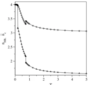
Figures 6 and 7 exhibit the fractions of hydrogen bonds and links per molecule as a function of temperature and pres-sure, respectively, atP = 0andT = 0. As expected, in both figures, the fraction of hydrogen bonds, which is pro-portional to energy, is a decreasing function of temperature, and presents discontinuities at the transition temperatures. In the region of constant pressure (Fig. 6) the fraction of links also decreases with temperature, except at the ID-HD phase transition, at which it shows an evident increase. This behavior can be seen from the fact that total entropy must increase with temperature: while the HD phase has a low spatial entropy (n6 = 1as can be seen in Fig. 4) the num-ber of links contributes to raise the entropy (eq. 16). For T = 0(Fig. 7) the fraction of links remains constant, with nc = 4, and the number of hydrogen bonds is maximum (4 in the LD phase and 8/3 in the HD phase), corresponding to the minimum energy configurations.
0 1 2 3 4 5 T
2 2.5 3 3.5 4
n HB, n c
Figure 6. Fraction of hydrogen bondsnH B(circles) and fraction of linksnc¯ (triangles) as a function of temperature atP = 0for a variable number of links. At the transition temperaturesnH B
changes discontinuously.nc¯ jumps in the second transition.
4 4.5 5 5.5 6 P
2.5 3 3.5 4
n HB, n c
Figure 7. Fraction of hydrogen bondsnH B(circles) and fraction of links ¯nc (triangles) as a function of pressure atT = 0for a variable number of links. At the transition pressurenH Bchanges discontinuously.nc¯ is constant, equal to4.
However, the diagram has some resemblance to that near the ice-Ih, where, for some values of temperature, the sys-tem goes from the ice-Ihto the liquid water and from this to the ice-V as the pressure increases[24]. These qualita-tive features are seen in our Fig. 3, at intermediate tem-peratures. The model cannot account for the liquid-vapor transition since the distance between the molecules is kept fixed. However, the increase in the density as the ture raises is akin to the behaviour of water at low tempera-tures.
Acknowledgements
MG and WF acknowledge financial support from the Brazilian agencies CNPq and FUNCITEC. NG and VBH
acknowledge financial support from the Brazilian agency Fapesp (NG 03/00831-8 and VBH 01/11721-3).
References
[1] F. Franks,Water, A Comprehensive Treatise(Plenum, New York, 1972).
[2] P. H. Poole, F. Sciortino, T. Grande, H. E. Stanley, and C. A. Angell, Phys. Rev. Lett.73, 1632 (1994).
[3] P. H. Poole, U. Essmann, F. Sciortino, and H. E. Stanley, Phys. Rev E48, 4605 (1993).
[4] W. L. Jorgensen, J. Chandrasekhar, J. D. Madura, R. W. Im-pey, and M. L. Klein, J. Chem. Phys.79, 926 (1983); M. W. Mahoney, J. Chem. Phys.112, 8910 (2000).
[5] H. E. Stanley, M. C. Barbosa, S. Mossa, P. A. Netz, F. Sciortino, F. W. Starr, and M. Yamada, Physica A315, 281 (2002).
[6] P. A. Netz, F. W. Starr, M. C. Barbosa, and H. E. Stanley, Physica A314, 470 (2002).
[7] D. Chandler, Nature417, 491 (2002).
[8] N. Guisoni and V. B. Henriques, Braz. J. Phys. 30, 736 (2000).
[9] N. Guisoni and V. B. Henriques, J. Chem. Phys.115, 5238 (2001).
[10] M. Girardi and W. Figueiredo, J. Chem. Phys. 117, 8926 (2002).
[11] W. Nadler and T. Krausche, Phys. Rev. A44, R7888 (1991); T. Krausche and W. Nadler, Z. Phys. B: Condens. Matter86, 433 (1992).
[12] E. H. Lieb, Phys. Rev.162, 162 (1967); E. H. Lieb, Phys. Rev. Lett.18, 692 (1967).
[13] J. D. Bernal, Nature185, 68 (1960); J. D. Bernal, Nature183, 141 (1959).
[14] H. Kawamura, Prog. Theor. Phys.70, 352 (1983).
[15] D. Yi-Jing, C. Li-Rong, and Y. Tzu-Tung, J. Phys. C: Solid State Phys.15, 3059 (1982).
[16] Y. M. Yi and Z. C. Guo, J. Phys. Condens. Matter1, 1731 (1989); Z. Guo and Y. Yi, Commun. in Theor. Phys.8, 17 (1987).
[17] R. Collins, Proc. Phys. Soc.83, 553 (1964).
[18] B. Rubinstein and S. I. Ben-Abraham, Mat. Sci. & Eng. A
294, 418 (2000).
[19] D. Joseph and V. Elser, Phys. Rev. Lett.79, 1066 (1997).
[20] M. Oxborrow and C. L. Henley, Phys. Rev. B 48, 6966 (1993).
[21] M. Widom, Phys. Rev. Lett.70, 2094 (1993).
[22] H. Kawamura, Physica A177, 73 (1991).
[23] W. L. Goffe, G. D. Ferrier, and J. Rogers, J. Econom.60, 65 (1994).