Printed in Brazil - ©2004 Sociedade Brasileira de Química 0103 - 5053 $6.00+0.00
Article
* e-mail: [email protected]
Thermal Conductivity of Gas by Pulse Injection Techniques Using Specific Thermal
Conductivity Detector (TCD)
Renato Cataluña*, Rosângela da Silva, Eliana W. Menezes and Dimitrios Samios
Instituto de Química, Universidade Federal do Rio Grande do Sul, Av. Bento Gonçalves, 9500, 91501-970 Porto Alegre - RS, Brazil
Este artigo apresenta um procedimento para determinar a condutividade térmica de gases através de injeção por pulso, utilizando um detector de condutividade térmica (TCD). As medidas foram efetuadas à 323K e pressão atmosférica, com um sensor de filamento de tungstênio de 160 Ω. Através de aproximações bem definidas, foi possível transformar uma equação de segunda ordem não-linear, que descreve a saída do sensor como uma função de condutividade térmica e calor específico a volume constante (Cv), em uma equação linear de primeira ordem. De acordo com esta equação, o sinal elétrico do sensor, elevado ao quadrado e integrado em função do tempo, multiplicado pelo Cv, é proporcional a razão do Cv pela condutividade térmica. Os resultados experimentais obtidos com os gases Ar, N2, O2, CH4, CO2, C2H4, C3H6 e i-C4H8 estão de acordo com o modelo teórico proposto e a correlação de linearidade confirma a validade do método proposto.
This paper presents a procedure to determine the thermal conductivity of gases by pulse injection, using a thermal conductivity detector (TCD). The measurements are taken at 323K and atmospheric pressure with a 160 Ω tungsten filament sensor. Under well defined approximations the original nonlinear second order equation, which describes the sensors output, as a function of thermal conductivity and constant volume specific heat was transformed into a linear first order equation. According to this equation the time integrated, second order sensors electrical output signal, multiplied by the constant volume heat capacity is proportional to the constant volume heat capacity, divided by the thermal conductivity. The experimental results obtained with Ar, N2, O2, CH4, CO2, C2H4, C3H6 and i-C4H8 gases are in good agreement with the proposed theoretical model and the linearity correlation confirms the validity of the proposed method.
Keywords: thermal conductivity of gases, thermal conductivity detectors, thermal conductivity procedure
Introduction
The thermal conductivity characterizes the capability of a compound to transfer heat. This transport, operating at the molecular level, is very variable according to the medium. The determination of the coefficient of the thermal conductivity is important for all calculations of heat transfer. However, there are no many instruments commercially available for measuring especially the thermal conductivity of liquids and gases.1 Davis et al.2
published a non-steady-state, hot wire, thermal conduc-tivity apparatus for fluids which has been tested with toluene. Clifford et al.3 have improved the accuracy of a
gas-phase thermal conductivity apparatus proposed by Haarmam.4 Imamuddin and Dupré5 treated the
mathe-matical aspects of the heat loss due to radiation in a thermal conductivity apparatus. Finally Lamoreux6 and Perkins et
al.7 have contributed for the instrumental improvement of
the thermal conductivity measurements.
In this paper we have used the evolution of the instrumental techniques and the informatics’ facilities to present a measurement method to estimate the thermal conductivity of pure gases and mixtures when the constant volume heat capacity is known. Thermal-conductivity detectors are commonly used as devices in gas chroma-tography to monitor individual substances separated in the column.8,9 These devices include the Pirani,
thermo-couple, and thermistor gauges, each of which can measure pressure and temperature by sensing changes in the thermal conductivity of ambient gases.10 According to the Fick´s
law11 the energy flux, caused by a temperature gradient, is
Jr(energy) = - κA (dT/dr) (1)
According to the kinetic theory of gases, the thermal conductivity, κA, of a perfect gas A with a molar
concentration [A] is given by the expression
κA =
1/
3λĉ CV,m[A] (2)
where λ is the mean free path, ĉ is the average molecular velocity of the molecules, and CV,m is the molar heat capacity at a constant volume.11 A rigorous treatment to
predict thermal conductivity of polyatomic fluids would require, therefore, a comprehensive knowledge of the separate and interactive behavior of translational, rotational and vibrational degrees of freedom of the polyatomic molecule.12 By using pulse method, two
different information namely, specific heat and thermal conductivity can be obtained within a single measurement.13
Additionally to experimental results we developed a new simplified theoretical approach, which permits to test the obtained experimental results for different gases and mixtures.
Experimental
The instrumentation of specific TCD
The general detection principle of thermal conductivity sensors is as follows. A known temperature difference is maintained between a “cold” and a “hot” element. Heat is transferred from the “hot” element to the “cold” element via thermal conduction through the carrier gas. A temperature gradient is established due to the thermal flow energy in the gas medium. The power required to heat the “hot” element, therefore, is a direct measure of the electrical signal output for the thermal conductivity. Heat loss due to radiation, convection and heat conduction through the terminals of the “hot” element must be minimized by sensor design.14
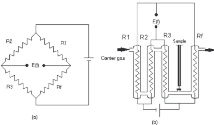
Figure 1 (a) illustrates the Wheatstone bridge and Figure 1 (b) the corresponding TCD device. The sensor consists of four chambers: a measurement chamber and three reference chambers. The chambers consist of borosilicate (Pyrex™) glass tubes having a 2 mm internal diameter and 40 mm length. Heating power is required to maintain the temperature difference between the “hot” element and the ambient temperature. The four chambers are located inside an aluminum block, which is equipped with an electronic control to keep the block and consequently the sensor’s temperature constant. Using helium, which possesses high
thermal conduction, as a carrier gas, the temperature of the filament is hold as low as possible. The carrier gas flux is 30 mL min-1, the injected volume of gas is 200 µL, the
temperature of the aluminum block is set at 323 K and the electric power supply is 14 V. The system operates to the constant pressure. When measurements are taken, the signal output of the voltage bridge is recorded continuously using a CIODAS-08 computer board. Measurements with a TCD are based on monitoring changes in the electric conductivity of the filament, caused by variation in its temperature during passage of the sample gas. The signal output “E(t)” in the Wheatstone bridge is based on changes in the resistance of the sensor “Rf”.
The proposed approach to estimate thermal conductivity using TCD
Under stationary conditions, the amount of heat transferred from the filament to the gas phase is proportional to the thermal conductivity of the flowing gaseous mixture and the difference in the temperature of the filament and the cell walls. The sensor’s temperature is constant under stationary heating conditions and a constant flow rate of an unchanging gas. In this case, the filament temperature remains constant and dTf(t)/dt=0. When a gas sample is injected into fluid flowing inside the duct, the transient filament temperature generates a transient voltage in the Wheatstone bridge E(t).
The thermal conductivity of the gas phase in the chamber sensor during the measuring experiment will be the result of the carrier and the gas sample. As thermal losses through the gas phase change, the temperature of the filament sensor will change as well. A change in the composition of the flowing gases is reflected in a change in the sensor’s temperature, causing a change in the sensor’s resistance, Rf, thus providing an electrically treatable signal.8 When an annular shell is set up around the filament
assuming that the filament’s temperature is uniform, the conductivity of the injected gas is isotropic in the x and r
directions, remaining constant with the temperature. Based on these assumptions, the proposed method allows one to obtain the following heat conduction equation:
– κgi S dTgi(t)/dr = n CvgidTgi(t)/dt (3)
where: dTgi(t)/dr = injected gas temperature space radial derivative; dTgi(t)/dt = injected gas temperature time derivative; Cvgi = constant volume heat capacity of injected gas; n = number of moles of injected gas; κgi =
thermal conductivity of injected gas; S = surface area of filament.
Assuming that the temperature gradient at the gas/ filament interface is linear and proportional to the difference between the temperature of the injected gas and that of the filament at time “t”, we can consider that:
S dTgi(t)/dr = C1 [Tgi(t) - Tf(t)] (4)
where: C1= proportionality constant; Tgi(t) = average temperature of the injected gas; Tf(t) = average temperature of the filament.
The following equation can therefore be written for each injection:
0
I∞Tf(t) dt –
0
I∞Tgi(t) dt = (n Cvgi/C1 kgi)
0
I∞dTgi(t) (5)
Measurements using the thermal conductivity detector are based on monitoring changes in the sensor’s resistance, Rf, since this resistance is a linear function of the temperature. The change in sensor temperature is measured as a change in the output voltage of the respective bridge circuit. If the Wheatstone bridge is perfectly balanced for a constant flow of carrier gas, the temperature of the filament related to the injected gas is proportional to the Wheatstone bridge’s signal output of the second order and the filament temperature is:
Tf(t) = C2 [E(t)]2 (6)
where, C2= proportionality constant; E(t) = output signal of Wheatstone bridge (Volts).
The temperature of injected gas can be expressed according to the following equation:
0
I∞Tgi(t) dt = Tgi(∞) - T0 = C3 ∆Tgi (7)
where we assume that Tgi(t) is a linear function of time; C3= proportionality constant; T0 = initial temperature of the
injected gas; ∆Tgi = temperature increment of injected gas.
0
I∞E(t)2
dt = F(n,Cvgi,κgi) = numerical integration of the
squared electrical output signal.
C2 F(n,Cvgi,κgi) - C3∆Tgi = (n Cvgi/C1 κgi) ∆Tgi (8)
F(n,Cvgi,κgi) = [(C3/C2) + 1/(C1C2) (n Cvgi/κgi)] ∆Tgi (9)
At this level of modeling, we have assumed that the integration of the electrical signal of the second power, F(n,Cvgi,κgi), of an injected gas is a function of number of
moles, specific heat and thermal conductivity of the injected gas. The temperature increment of injected gas,
∆Tgi, decreases as the number of moles and heat capacity increase. Thus, considering that ∆Tgi is a function of the number of moles and heat capacity, it follows that:
∆Tgi = C4/(Cvgi n) (10)
where C4 is the proportionality constant.
Combining the above with the numerical integration of the second order signal output, F(n,Cvgi,κgi), for the same
injected volume, one obtains:
F(Cvgi,κgi) = a/Cvgi + b/κgi (11)
where “a” and “b” are adjusted constants.
The evaluation of the proposed approximation
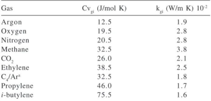
In order to evaluate the proposed approximation, nine pure gases and one mixture were used. Table 1 shows the constant volume heat capacity and the thermal conductivity15 of the gases used in the experimental test.
Results and Discussion
The results of the time integrated, second order sensors electrical output signal, in V2, as shown in Table 2, are the
Table 1. Constant volume heat capacity and Thermal conductivity of used gases
Gas Cvgi (J/mol K) kgi (W/m K) 10-2
Argon 12.5 1.9
Oxygen 19.5 2.8
Nitrogen 20.5 2.8
Methane 32.5 3.8
CO2 26.0 2.1
Ethylene 38.5 2.5
C4/Ara 32.5 1.8
Propylene 46.0 1.7
i-butylene 75.5 1.6
aC
mean values of ten consecutive injections performed for each gas in a test in which the injections were made in the sequence presented and thermal conductivity obtained from the mean value. After the first test, the equipment was turned off, allowed to cool, and then set to the same conditions, whereupon new injections were made following the same sequence.
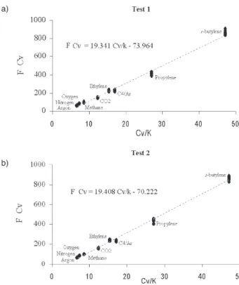
The results depicted in Figure 2 represent ten consecutive injections for each gas or mixture. As can be seen in the results of Table 2, the thermal conductivity values obtained experimentally from the mean values of
the electrical signals output in the second test were slightly lower than those literature data presented in the Table 1. Moreover, as the specific heat increases, so did the signal, indicating that the filament’s temperature was highly susceptible to the specific heat of the gas. As the specific heat increases, the transmission of heat from the filament to the gas phase decreases. Of all the gases analyzed here, methane displayed the highest thermal conductivity; however, it showed the lowest relative response to the filament’s temperature. A slight increase in the temperature of the injected gas, ∆Tgi, reflects a low heat transmission, leading to a higher filament temperature and, hence, to a stronger signal.
However, the temperature of the filament for CO2, ethylene, propylene and i-butylene increased substantially due to a greater contribution to vibrational modes. This, of course, is not possible for the monoatomic Ar and is less pronounced in methane.16
Conclusions
A procedure was proposed to determine thermal conductivity of gases when the heat capacity is known. The method proposed here is based on a set of nonlinear equations of the measured signal output in a Wheatstone bridge.
It was found that different gases with known thermal conductivity and heat capacity are needed to adjust the constants of the equipment. The results demonstrated that the standard deviation of the mean signal outputs were quite small. The congruence between the proposed equation and the experimental results confirms that the method accurately determines the thermal conductivity.
A drop in the sensor’s temperature was observed when it was exposed to gases with high thermal conductivity and low heat capacity. The negative value of the linear coefficient “a” observed in the experimental results is in Table 2. Two tests with experimental mean values of the time integrated, second order sensors electrical output signal, the standard deviation and thermal conductivity values obtained from ten consecutive injections for each gas
Test 1 Test 2
Gas Average κgi (W/m K) 10
-2 Average κ
gi (W/m K) 10 -2
Argon 4.95±0.12 1.8 5.26±0.15 1.8
Oxygen 3.65±0.09 2.6 3.83±0.12 2.6
Nitrogen 4.09±0.14 2.5 4.22±0.12 2.5
Methane 3.06±0.13 3.6 3.09±0.06 3.7
CO2 5.90±0.16 2.2 6.05±0.15 2.2
Ethylene 5.92±0.19 2.5 6.19±0.16 2.4
C4/Ara 7.07±0.23 2.1 7.21±0.13 2.1
Propylene 9.11±0.30 1.8 9.31±0.42 1.8
i-butylene 11.4±0.30 1.6 11.5±0.30 1.6
aC
4/Ar is a gas mixture of 66% argon and 34% i-butylene.
Figure 2. Relation between Cvgi/κgi and output signal F(κgi, Cvgi)
agreement with the theoretical model, which states that the signal output increases concomitantly to increased heat capacity.
References
1. Parlouer, P. L.; Rouyer M.; Pithon F.; Thermochim. Acta 1985,
92, 375.
2. Davis, P. S.; Theeuwes, F.; Bearman, R. J.; Gordon, R. P.; J. Chem. Phys. 1971, 55, 4476.
3. Clifford, A. A.; Colling, L.; Gray, P.; Tong, D. A., Tough, G. S.; J. Phys. E: Sci. Instrum.1974, 7,283.
4. Haarman, J.W.; Physica 1971, 52, 605.
5. Imamuddin, M.; Dupré, A.; J. Phys. E: Sci. Instrum.1976, 6, 540.
6. Lamourex, R. T.; Thermochim. Acta1979, 34,127.
7. Perkins, R. A.; Roder, H. M.; Decastro, C. A. N.; J. Res. National Institute of Standard and Technology 1991, 96, 247.
8. Sevcik, J.; Detectors in Gas Chomatography, Elsevier Scientific Publishing Company: Amsterdam, 1976, p. 39.
9. Sorge, S.; Pechstein, T.; Sens. Actuators, A 1997, 63, 191. 10. Klaassen, E. H.; Kovacs, G. T. A.; Sens. Actuators, A 1997, 58,
37.
11. Atkins, P. W.; Physical Chemistry, Oxford University Press: Oxford, 1998, p. 724.
12. Lielmezs, J. and Herrick, T. A.; Thermochim. Acta 1989, 141, 113.
13. Kubicar, L.; Illeková, E.; Thermochim. Acta1985, 92, 441. 14. Simon, I.; Arndt, M.; Sens. Actuators, A2002, 97-98, 104. 15. Perry, R. H.; Green, D. W.; Perry’s Chemical Engineers’
Handbook, Mc Graw Hill: New York, 1984, p. 3.
16. Kouber, E.; Braun, C.L, Juergens, F.; Chem. Educ. 1986, 63, 267.
Received: September 16, 2003