Furthe r analysis o f o pe n-re spiro me try
syste ms: an a-co mpartme ntal
me chanistic appro ach
Departamento de Fisiologia, Instituto de Biociências, Universidade de São Paulo, São Paulo, SP, Brasil J.G. Chaui-Berlinck and
J.E.P.W. Bicudo
Abstract
A system is said to be “instantaneous” when for a given constant input an equilibrium output is obtained after a while. In the meantime, the output is changing from its initial value towards the equilibrium one. This is the transient period of the system and transients are important features of open-respirometry systems. During transients, one cannot compute the input amplitude directly from the output. The existing models (e.g., first or second order dynamics) cannot account for many of the features observed in real open-respirometry systems, such as time lag. Also, these models do not explain what should be expected when a system is speeded up or slowed down. The purpose of the present study was to develop a mechanistic approach to the dynamics of open-respirometry systems, employing basic thermodynamic con-cepts. It is demonstrated that all the main relevant features of the output dynamics are due to and can be adequately explained by a distribution of apparent velocities within the set of molecules travel-ling along the system. The importance of the rate at which the molecules leave the sensor is explored for the first time. The study approaches the difference in calibrating a system with a continuous input and with a “unit impulse”: the former truly reveals the dynamics of the system while the latter represents the first derivative (in time) of the former and, thus, cannot adequately be employed in the apparent time-constant determination. Also, we demonstrate why the apparent order of the output changes with volume or flow.
Co rre spo nde nce
J.G. Chaui-Berlinck Departamento de Fisiologia Instituto de Biociências, USP 05508-900 São Paulo, SP Brasil
Fax: + 55-11-818-7422 E-mail: jgcb@ usp.br
Research supported by a FAPESP grant to J.E.P.W. Bicudo. Part of a PhD thesis presented by J.G. Chaui-Berlinck to the Departamento de Fisiologia, Instituto de Biociências, Universidade de São Paulo, and supported by a CAPES fellowship.
Received June 23, 1999 Accepted March 10, 2000
Ke y words
·O pen-respirometry systems ·Thermodynamic model
Intro ductio n
The dynamics of a respirometry system is an essential feature of such a system and investigators must be fully familiarized with it before experiments begin. This is due to the fact that respirometry systems have tran-sients, i.e., periods of time during which the output amplitude (the signal) of the system is below the amplitude of the input. Therefore, during transients, one cannot compute the
transform the output into instantaneous read-ings by some mathematical procedure (1), i.e., to obtain output amplitudes linearly re-lated to the input amplitudes. Three branches of such solutions are found in the literature: a) single-chamber first-order models (2-10), b) two-chamber second-order models (11), and c) unknown number of chambers free-of-order models (12,13). The first-order models analyze the output as coming from a single volume of dilution, and the Z-trans-formation of the output is the mathematical procedure used to obtain instantaneous read-ings (4) even though adding the output to its first derivative in relation to time is another possibility (7-9). Free-of-order models em-ploy deconvolution of the output by a trans-fer function obtained during calibration pro-cedures. The putative number of volumes diluting the input is irrelevant to this trans-formation, and the procedure is simply in-strumental in this respect.
Frappell et al. (11) proposed a two-cham-ber model that resulted in a second-order solution. They stated the superiority of their model in relation to first-order ones based on the fact that the second-order function pro-file is much more similar to empirical output profiles than are first-order function pro-files. Several flaws can be detected in their model, and we list them in Appendix A (see page 979). One of these flaws (perhaps the most relevant one) is the statement that the profile of the output will approach a first-order dynamics if the first chamber is large in relation to the second one (or vice-versa). Empirically, one can demonstrate that the larger the volume of a chamber the less the output is close to a first-order model (see Figure 5A). This phenomenon is not related to an a priori predetermined number of cham-bers counted from an anthropocentric point of view.
Let us state the problem in another way. Consider a given system1 Syst1 with an out-put that apparently obeys a given order (e.g., N order). Then, increasing the volume of such a system or decreasing the convective flow through it (i.e., slowing down the sys-tem) would result in a) a system (Syst2) that is of the same N order as Syst1 but with different values for the time constants that describe it, or b) a change in the order of Syst2 in relation to the apparent N order describing Syst1. Mutatis mutandis, the ques-tion holds true for the opposite, i.e., when a system is speeded up. Empirically, we al-ready know that a change in the order of the apparent function describing the output will occur. However, none of the present models explains why and how this happens to be so. These models also cannot account for the so-called “time lag” (i.e., a finite amount of time between the input taking place and some alteration occurring in the sensor cell)2. All these problems are present in such mod-els because the latter are not truly describing the mechanics of the systems. Instead, they are fitting a pre-set of differential equations to the observed output.
In the present study we developed an approach to open-respirometry system dy-namics employing basic concepts of thermo-dynamics and statistical mechanics. This approach allows an unequivocal understand-ing of the principles underlyunderstand-ing the relation-ship between volume and flow in open-res-pirometry systems, thereby clearly explain-ing why and how there is a change in the apparent order of the output when a system is speeded up or slowed down. We also explore the role of the sensor cell itself in the system and the difference between calibrat-ing an open-respirometry system (i.e., how to obtain its dynamics) by a continuous input and by a unit impulse.
Me thods and Re sults
The basic e xpe rime ntal se t-up
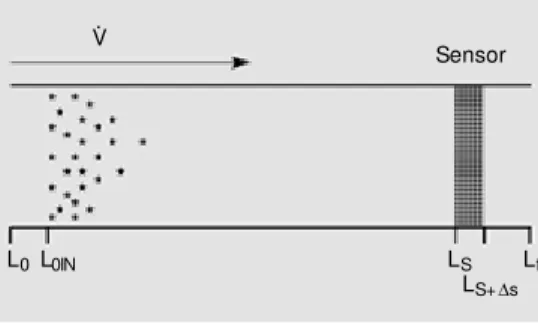
Appendix B (see pages 979 and 980) contains a list of symbols and definitions. We describe here the main features of open-respirometry systems. These systems consist of tubes connected to each other in series. The system is said to initiate at the L0 point, i.e., the point where the system starts physi-cally (before L0 is the outside environment). The series of connected tubes reaches the entrance of the sensor cell, S, at LS. The sensor cell has a given volume and ends at a point called LS+Ds. Finally, the system ends at
a point called Lf: beyond Lf there is, again, the outside environment. There is a convec-tive flow, V., of ambient gas through the system from L0 to Lf. V. determines a sense of convective flow within the system, defined as the x+ (x positive) sense. The input into the system occurs at a point called L0IN. For practical reasons we will simply state that L0IN>L0, i.e., the input occurs beyond the entrance to the system, in the x+ sense. The connected tubes consist of a volume which, from the “output point of view”, extends from L0IN to LS+Ds (not just to LS) as we will
demonstrate below. The gas molecules of the input flow through the system from L0IN. Figure 1 illustrates the main features of open-respirometry systems. For the sake of sim-plicity, but without loss of generality, the following constraints are part of this ap-proach: a) temperature is constant; b) the cross-section of the connected tubes is con-stant; c) the sensor cell has the same cross-section as the other tubes; d) the external environment acts as an infinite pool and sink; e) all gas molecules have the same mass and diameter, and collisions are elas-tic; f) the system is in a steady-state of pres-sure, i.e., the transients of the convective flow have finished, and g) there is no input loss (this is why L0IN>L0) and turbulence will not be accounted for in the approach.
If all molecules had the same velocity in the x+ sense of the system the output of any given input would look like a square pulse. However, in real systems, this is not the case, because the input molecules do not have all the same velocity, as will be demonstrated below.
Re al ve locitie s of the particle s - total and the X component
At any given temperature (greater than 0 K) the distribution of velocities in a popula-tion of gas molecules follows a Maxwell distribution (14):
2
M v
2 2RT
(v)
M
f
4
v e
2 RT
(1)
where M is the molar mass of the molecules, R is the gas constant, T is temperature and v is the specified velocity of a population f of molecules (Figure 2A). At any Lj point along the system (L0<Lj<Lf) the profile of veloci-ties described by equation 1 is expected to be found. Consider now a step change in the input that occurs at t0 (t0 is the exact moment when a transition in the amplitude of a former constant input occurs). This new input is composed of a set of molecules whose ve-locity profile is described by equation 1 as well, and this set of molecules shows this profile at any observation time (given that we are considering a conservative system, item (a) above). However, this does not mean that each molecule in the set is locked in a fixed velocity. On the contrary, each time a molecule collides its velocity changes. Thus,
Sensor V.
L0L0IN LS
LS+Ds
Lf
Figure 1 - Schematic view of an open-respirometry system. The input takes place at L0IN, and the
gas particles (represented by as-terisks) travel from this point to the end of the system, Lf, under a
convective flow V.. During the travel, the gas particles pass through a sensor that begins at LS and ends at LS+Ds. The entry of
the system is identified at L0, a
each molecule tends to reach a mean ve-locity due to collisions. Over time, the set of these molecules can be described as having a mean velocity c-(t) (the mean velocity of the Maxwell distribution: c-(t) = 8RT M al-though the profile of the set (given by equa-tion 1) is the same at any particular time. This mean velocity has a standard deviation,
(t)
c mxw
sd
sd
collisions
, where sdmxwis the standard deviation of the original (Max-well) distribution divided by the square root of the number of collisions of the particle from t0 to t (the result for sdc-(t) is simply the Law of Large Numbers or central limit theo-rem (15)). Due to the huge number of colli-sions a particle suffers within short periods of time (see below) we will simply use sdc-and c- instead of sdc-(t) andc-(t), respectively.
700 600 500 400 300 200 100 0 N um be r of p ar tic le s
200 400 600 800 1000 Velocity 800 % P op ul at io n 0.0025 0.0020 0.0015 0.0010 0.0005 0.0000
0 0 200 400 600
Velocity A B 1200 1000 800 600 400 200 0 N um be r of p ar tic le s
20 40 60 80 100 Number of collisions
480 V el oc ity o f a pa rt ic ul ar m ol ec ul e 800 600 500 400 200 100
0 320 360 400 440
Velocity
C D
300 700 Figure 2 - Gas particles tend to
reach a mean velocity as colli-sions occur. A, M axw ell distri-bution of velocities in a gas sample at 300 K. B, 10,000 par-ticles w ere fitted w ithin the M axw ell distribution show n in A. C, Change in velocity of a simulated particle as collisions take place. The dashed line rep-resents the mean velocity the set w ill tend to reach. D, The 10,000 particles of B w ere al-low ed to change velocity at ran-dom (under the constraint of constant temperature, i.e., the velocit ies f ound in B w ere shuffled among the particles) during episodes of putative colli-sions. The mean velocity of each of the 10,000 particles w as re-corded and the result of these means after the 100th collision episode is show n. Note the clear tendency tow ards a normal dis-tribution of the velocities (from B to D; also note the different scales). Velocity is in m/s.
Therefore, a gaussian curve adequately de-scribes the velocity profile of the particles in a given initial set:
2 c 1 v-c -2 sd v c
1
G
e
sd
2
(2)in the very first second after the input takes place. Figure 2 illustrates these points.
Thus, it was shown that the total velocity, v, tends to reach a mean value for each particle as time goes by. This total velocity is the vector composed by the three orthogonal components of velocity:
2 2 2 2
x y z
v
v
v
v
(3)These orthogonal components are inde-pendent of each other, i.e., changes in one of them do not imply changes in the other ones (as long as the temperature is constant and, therefore, the total kinetic energy of the ini-tial set is constant (14)). We are concerned with the travelling rate in the x direction, i.e., with the speed of the particles going from L0IN to LS+Ds. The distribution of velocities
on a given axis (e.g., x) is:
2 x
x
M v 2RT (v )
M
f
e
2 RT
(4)
With time, each molecule in the initial set attains a mean velocity on such an axis, and, as seen before, the set can be described as having a mean velocity on the axis (c-x) and a standard deviation of this mean (sdc-x):
2
x x
cx x
x
v -c 1
-2 sd v
c
1
G
e
sd
2
(5)
It should be noted that equation 5 describes the mean velocity in the x direction (or any other orthogonal axis), but is blind to the sense of the motion (i.e., it represents both the positive and the negative components in the given direction). We will now consider what happens when convective flow is pre-sent.
Appare nt ve locitie s of the particle s
Gas particles are in a constant rocking motion, coming and going all the time. They
collide with each other and, at such colli-sions, they can change the sense of their motion (e.g., from a positive x sense to a negative one). When convective flow is im-posed on the system, there is nothing that really pushes or pulls each particle. Instead, there is a higher probability that a particle once moving in the positive sense of the flow (as defined above) will continue in such a sense longer than when it is moving in the opposite one. Given that changing in the sense of the motion only occurs when par-ticles having opposite senses collide, we can write the difference in probability that a particle would change sense at a given point Lj of the system as:
(Lj)
(Lj)
(Lj)
z
1
z
(6)
where z stands for the collision frequency that a particle experiences at Lj when travel-ling in the positive (z+) and in the negative (z-) sense of the x axis. Thus, when collision frequency is the same in both senses (no convective flow is present) L = 0, i.e., only the probability of diffusion affects the move-ment of particles from one point to another. A good approximation for L (as we justify in Appendix C (see pages 980 and 981)) is:
X
w
c
(7)where Dw is the absolute value of the ve-locity of the moving piston causing convec-tive flow and c-x is the mean velocity of the particles in the x direction. Notice that L is independent of the Lj point of the system. The apparent velocity (in the x direction) of a particle will be the product of its mean velocity and L. Therefore, the whole set has a mean apparent velocity indicated by the following equation:
app
x X
A note on variance: many factors were not taken into account in this study. Some of them are turbulence, inhomogeneities of the gas medium, changes in the geometry of the tubing, and the variance in L. Analysis of such factors is beyond the scope of the pres-ent study. However, it is very important to note that these added variances make a con-siderable contribution to the final spreading of velocities around the mean value.
We will not propagate error and the standard deviation of the above apparent mean velocity will be simply described as sdapp+ =
sdc-x.L, where the superscript + indi-cates that added components of variance should be included. Normality is preserved3 and the set of particles can be adequately described by a gaussian function as:
Equation 9 is the foundation of this study. It tells us that any given initial set of particles will attain a mean apparent velocity on the axis of the convective flow imposed on the system, and that particles of such a set will have apparent velocities normally distrib-uted around the mean velocity of the set. This obviously explains, unequivocally, the existence of the time lag between an input and the beginning of the corresponding out-put: it is the length of time that the faster particles of the input take to travel from L0IN to LS (even though a gaussian function ranges from -¥ to +¥, for practical purposes the entire population can be considered to lie between -3sd and +3sd around the mean, so there will exist a minimum time required for the faster particles to travel). In the next section we will explore the output dynamics that results from equation 9.
O utput dynamics of open-respirometry syste ms
The input. Most of the arguments of the functions will be omitted for the sake of simplicity (e.g., G instead of G(vxapp)). Let us consider a set A of gas molecules as an unitary amplitude input into the system. Therefore, such a set has particles which have velocities distributed according to func-tion G (equafunc-tion 9). Obviously, set A has a total number of molecules corresponding to the integral H of G (because the velocities in this case are equal to or greater than zero, the integral will be evaluated only in the positive range):
total particles of A = H = 2
The total amount of molecules in a con-tinuous input into the system at time t is the integral of A in relation to time, from t0 = 0 to t:
t 0
H
t H
dt
(11)The output. Let us define a function E(t) representing the state of the sensor at time t. The state of a sensor is a function (linear, in general) of the occupancy level of the sensor by the subject of measurement of that sensor. The entry rate into the sensor is the amount of molecules (subject of meas-urement) that cross the entrance to the sen-sor cell at LS. The exit rate is the amount of molecules leaving the sensor cell at LS+Ds:
s+ s
s s+ s s
L t (t)
L L L
t t t
E
G
G
G
dv
dv
dv
3And this is true because these errors are normally distributed as w ell.
2 xapp xapp
app xapp
v -v 1
-2 sd v
app
1
G
e
sd
2
(9)
(10)
Therefore, the output dynamics of an open-respirometry system, equivalent to the state E(t) of the sensor, is only a function of the velocities of the particles of the input travel-ling a linear distance to reach the entrance and then the exit of the sensor. The apparent mixing or dilutional features of these sys-tems are just the result from the difference in the time of arrival, at the sensor, of the particles of a given input set (see below). This was never taken into account before. By examining equation 12 we can see that when
s
L t
G
dv
=s+ s
L t
G
dv
i.e., roughly speaking, when the exit rate equals the entry rate, E
.
(t)= 0 and so, E(t) = constant. At that time, the output stabilizes at a level, and such a level is the same as the amount of molecules coming from a corre-sponding time interval at the input (see equa-tion 10). In other words, the output becomes linearly related to the input.Another point that was also never appre-ciated before is that the leaving rate of the gas molecules from the sensor is crucial to the output dynamics. To stress such a point, consider a very long sensor (in the x direc-tion), in a way that
s
L t
G
dv
= Hat a time t when
s+ s
L t
G
dv
= 0i.e., the entry rate attains a stable value at a
time when the exit rate still equals zero. Roughly speaking again, the slowest subset of molecules enters the sensor while the fastest subset has not reached the exit of the measuring device. Under these conditions, the output becomes a linear function of time (from equation 11, E(t) = t.H)4! This would be impossible to understand using other cur-rent models interpreting the output of open-respirometry systems. Even when the sensor is not that long some linear component can be present, arising from the slower subset(s) of molecules.
Particular solution for a small measur-ing device. Let us consider a very short sensor (in relation to the convective flow employed), where LS @ LS+Ds, and let us state
without proof that this happens to be the most usual finding in open-respirometry systems. Thereby, the integral of equation 12 be-comes (see Appendix D, pages 981 and 982):
s
(t) (t)
L t
E
G
H
dv
(13)Equations 12 and 13 are useful to ap-proximate the real output. Thus, the deriva-tive of the output of the system is the distri-bution function of the apparent velocities of the particles (equation 9), and the output itself is the integral of that gaussian function. Figure 3 illustrates numerical solutions of equation 12 and equation 13 for constant input in systems with different volumes (no-tice that volume is the linear distance from L0IN to LS) under the same convective flow (apparent velocity of the particles). Notice how the profiles of the output suggest the existence of dilutional spaces (volumes) dic-tating the dynamics of the systems.
Increas-4Until molecules reach the outlet boundary and thus begin to leave the sensor. Note that this linearity is completely
ing the volume of the system (i.e., increasing the linear distance from L0IN to LS) appears to increase the number of “volumes” diluting the output, and this will be discussed below. However, before approaching this subject we will examine another common calibration pro-cedure, the “unit impulse”. In this technique, a set of particles A makes up a unique input which occurs within an interval of “zero” units of time. Therefore, as in equation 10,
0
total particles of
H
2 G
dv
Thus, the output, when integrated over time,
results in H, and as a consequence5:
s+ s
s
L t ui (t)
L t
E
G
dv
(14)
where the superscript ui stands for “unit impulse”. Notice that the output of a unit impulse (equation 14) corresponds to the first derivative in relation to time of a con-tinuous input (equation 12). When the time constants of a given system are determined using an exponential decay model (as the current models) there would be little distor-tion in such constants, because the expo-nents in those decays are the same in both the integral and its derivative. However, authors overlook the ascending portion of E(t)ui 6 (see
Figure 3A and next section) and look only at the descending (“exponential decay”) part of the curve. Time constants are then ad-justed to this descending portion of the curve. This can lead to serious distortions in the reconstituted experimental inputs.
Change in output “orde r” with the slowing down or the spe e ding up of open-respirometry systems
This section is devoted to the problem stated in the Introduction of this study: in-creasing the volume of a Syst1 system or decreasing the convective flow through it (i.e., slowing down the system) would result in a Syst2 system that is of the same order as Syst1 but with different values of the time constants describing it, or would there be a change in the order of Syst2 in relation to the apparent order describing Syst1? We will demonstrate that the latter alternative is the case. Firstly, we will approach the causes leading to a change in the apparent order of
5We are still w orking w ith the constraint of a very short sensor.
6Do they consider that the peak of the curve corresponds to the total amplitude of the unit impulse input itself?
d
E
/
d
t
0.08
0.06
0.04
0.02
0.00 a
b
c
d
a b c
d
E(t)
(
re
la
tiv
e
am
pl
itu
de
)
1.00
0.75
0.50
0.25
0.00
0 2 4 6 8 10
Time (arbitrary units)
0 2 4 6 8 10
Time (arbitrary units) Figure 3 - Numerical solution of
E
.
(t) and E(t) (equations 12 and13, respectively). Parameters w ere (in arbitrary units): mean velocity = 200, standard devia-tion = 50. The soludevia-tions w ere computed for 4 different puta-tive volumes of the system, i.e., 4 different distances from L0IN
to LS. (a = 100, b = 250, c = 500,
d = 1000). The sensor volume w as fixed as 5 arbitrary linear units (i.e., LS+Ds - LS = 5). A, Solutions of E
.
(t). As the volumeis increased,E
.
(t) attainsprogres-sively low er values. The profile of E
.
(t) for a continuouscalibrat-ing input turns into the profile of E(t) for a unit impulse calibrating
input (see text). There is an as-cending part of the curves that is truly part of the output, and cannot be slight w hen “ time constants” are computed for unit impulses (see text). B, Solu-tions of E(t). The outputs of the
different volumes (a, b, c, and d) are show n, w ithout time lag cor-rection. Using the same time scale of data acquisition, an in-crease in the order of the sys-tem w ill appear to occur from a to d and, thus, more time con-stants should be added (see text).
A
the output dynamics occurring in a system that is being described by a single time con-stant, i.e., a putative first-order output. Then, we will extend the conclusion to any given apparent order of open-respirometry systems. Throughout the analysis it is necessary to bear in mind that we are considering func-tions which tend to an asymptotic value as time goes by. Thus, any pair of vectors repre-senting such functions will tend to have norm®0 as t®¥ simply because they both tend to stabilize at a certain value. Therefore, in the following reasoning, we are concerned only with the period of time within which transients are present. In a general form: 0 = t0£t£T, where t0 = 0 is the time when the output begins to be detected and T is a later time when the total amplitude of the output is attained, on practical grounds. Note that t0 in this section has a different meaning from that used in the preceding ones, because it is not the initial time at which the input takes place.
Consider a Syst1 system where ||Y1(t). H1(t)|| = e1 (where ||w1.w2|| is the norm be-tween two vectors w1 andw2), and one tends to accept function Y as a good approxima-tion to H within an e1 error. The Y function has the general form shown below (equation 15).
Proposition: given a system with output H1(t) (H(t) is found in equation 13) for which an approximation Y1(t) @ H1(t) (within an error e1) is considered valid, the progressive increase of LS7 or decrease of V. will always result in ||Y2(t).H2(t)||>e1 with H2(t)<<Y2(t) for all t<tcross (to be defined below). That is, at the beginning of the output, the approxi-mating (new) function Y(t) has values pro-gressively greater than those of the real H(t) function as a given system is slowed down.
Demonstration. Let functions f1 and f2 be:
(t)
s
(t)
1 (t)
L
t (t)
t
2 (t)
f
H
G
f
Y
1 e
dv
(15)
where l is the inverse of a time constant. One intends to minimize
(t) (t)T 2
1 2
0
f
f
(let this function be f3) by varying l. The traditional method to do so is to find the value of l for which
.
Resolving the square and taking the first derivative of f3 in relation to l, one obtains the following result:
T T T - t
(t) (t) 0 0 0
1-e G Y - H 0
dv (16)
Therefore, because there are no squares in either term of equation 16, it becomes im-plicit that part of the values of Y(t) must be higher than the corresponding H(t) and an-other part must be lower for the sum to result in zero (unless Y(t) º H(t), see below). If Y(t) º H(t), it follows that
Y
H
t
t
, but:
s
v
L v 1 t 2 sd - t
(t) v
1
e
e
G
sd
2
(17)
7The linear distance from the input to the entrance of a very short sensor (see above) directly related to the volume
invalidating the putative Y(t) º H(t). The crossing time of G(t) and l.e-l.t , tcross
¶,
is:
3 2 2
cross v v
2
2 s s
cross 2 cross 2
v v
t
ln
sd
2
v sd
2 v L
L
t
t
0
sd
sd
The initial conditions are:
Y0 = H0 = 0 (19)
So:
G
(t) < l.e
-l.t , " t < t
cross¶ (20)
Let us define tcross (tcross>0) as the time when Y(t) and H(t) cross each other after their initial crossing at t0 = 0 (equation 19). It follows that Y(t)>H(t) for all t<tcross, that is, the solution of the minimization (equation
16) implies that the initial part of the ap-proximating function Y(t) has higher values than the real function H(t). Because tcross¶ is
directly proportional to LS (equation 18) and equation 16 is a minimization, then Y2(t) (for all t<tcross) is progressively higher than H2(t) as LS is progressively increased (and the same is valid for decreasing V. ), irrespective of wether the computed value l28 satisfies equation 16 or any other metric minimiza-tion procedure. In other words, as an initial system 1 in which it is accepted that Y1(t) @ H1(t) is slowed down and becomes system 2, the approximating function Y2(t) has greater values than the real function H2(t) from t = t0 until their crossing at a later time (tcross). The vectors representing the functions fall pro-gressively apart. At the beginning of the output, the error e2 is greater than the for-merly accepted e1 for the same period. This phenomenon, under compartmental analy-sis, emerges as the necessity of adding more “dilutional volumes” to a sum of exponentials (i.e., more time constants in order to “slow down” the initial part of the approximate function).
Consider any output H(t) being described (by approximation) by a function Y(t) in the general form
i
n t ( t )
1
Y
e
.
Any li represents a relationship between a putative “dilutional volume” and flow. Thus, the above reasoning extends to any number of time constants employed to describe the output of a given system. This reasoning demonstrates the obligatory change in the apparent order of the system output, and, therefore, the impossibility of a given order be the same as open-respirometry systems are speeded up or slowed down. Note that the definition of volume (LS) is not
anthro-8The time constant of Syst2, a slow ed dow n system in relation to Syst1.
F G
DRY
C S
Figure 4 - Schematic view of the system employed to collect empirical data. The convective flow (F) of ambi-ent gas passes through a pre-chamber (G), through a drying chamber (DRY), and through the chamber (C), and then reaches the sensor (S, oxygen sensor AM ETEK S-3A/I; Pittsburg, PA, USA). After stable out-put w as obtained, a constant inout-put w as added to the pre-chamber, thus generating a deflection in output. The volume of chamber C could be changed in the parallel axis of the flow , w hich in turn could be changed as w ell. The volume of the drying chamber and con-necting tubing corresponds to less than 5% of the minimum volume of C. Chambers w ere made using connected PVC tubes (commercially available), silica (Sigma Chemical Co., St. Louis, M O, USA) w as used to fill the drying chamber and air w as continuously pumped through the chamber at different flow rates, depending on the testing procedure (outlet measure-ments of flow , FL-1495-G flow meter, Omega Engi-neering, Inc.; Stamford, CT, USA).
pocentric, i.e., we are not “counting cham-bers”. Instead, LS is a continuum measure, blind to “chamber” definitions.
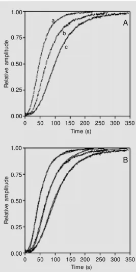
Some experiments were done in order to illustrate the points demonstrated above: a) the change in the apparent order of output as volume and flow are changed, and b) that this is not linked to the number of “cham-bers” from an anthropocentric viewpoint. Figure 4 shows the system employed. Note that there is a single chamber whose volume can be increased or decreased on the parallel axis to the convective flow, which in turn can be increased or decreased as well. Figure 5 presents the empirical results obtained by changing volume or flow in the system de-scribed above. Also, numerical evaluations of integrals of the general form of equation 13 are shown. Notice the fine adjustment between empirical data and the predicted functions (see legend).
Discussio n
Transients are important features of open-respirometry systems. Whether they are de-tected or not in real data acquisition proce-dures is a question that has to be known beforehand by the researcher. In cases where transients are detected, and the input is to be evaluated during such transients, the dynam-ics of the output is a major problem. In this study we employed basic concepts of ther-modynamics and statistical mechanics to de-velop an approach to the problem of the output dynamics of open-respirometry sys-tems.
The main result of this mechanistic ap-proach is that molecules of the input travel a linear distance from the place where such an input takes place to the sensor, with an ap-parent velocity normally distributed around a mean value (function G in equation 9). All the important features of the output dynam-ics are determined by this travelling rate of the molecules which end up reaching and leaving the sensor cell at different times.
This is the observed dynamics. Once this is recognized and quantified, time lag (the time between the beginning of input and the time where something begins to be detected at the sensor) becomes easily and unequivocally explained. Other current models cannot ac-count for such an explanation. This study also revealed that the rate at which the mol-ecules leave the sensor cell is an important part of the observed dynamics, a fact never considered before. This leads to a particular solution to the output for “very short sen-sors” (equation 13). Unless such a particular solution can be applied to a real experimen-tal set-up, the presence of linear components in the output should be expected, and the current exponential approaches would be inherently inappropriate.
Figure 5 - Empirical data ob-tained in the system shown in Figure 4. A, Output from 3 dif-ferent combinations of system volume and convective flow: a = (V. = 2.2 ml/s, volume = 200 ml), b = (V. = 0.8 ml/s, volume = 100 ml), c = (V. = 0.8 ml/s, vol-ume = 200 ml). Plots were time lag corrected. B, The same data as shown in A plus numerical solutions of E(t)º H(t). E(t) for the
different com binations w as computed as follows: a = (mean velocity = 263.2, standard de-viation = 65.9, LS = 22200), b =
(mean velocity = 120.5, stan-dard deviation = 30, LS =
16200), c = (mean velocity = 120.5, standard deviation = 30, LS = 22200). Note that the ratio
between the mean a:b veloci-ties is less than the ratio be-tween the a:b flows, probably due to measurement errors and non-linearity in flow (e.g., turbu-lence). Also, the ratio between LS from b and c is greater than
the volume ratio (100/200) due to the subsets of particles that have greater velocities and are therefore detected by the sen-sor sooner than expected by the volume ratio (compare to the curves shown in Figure 3B). The agreement betw een real and computed data is extremely evi-dent, w ith r2>0.95 for all the
three data sets.
R
el
at
iv
e
am
pl
itu
de
1.00
0.75
0.50
0.25
0.00
0 50 100 150 200 350 Time (s)
300 250
R
el
at
iv
e
am
pl
itu
de
1.00
0.75
0.50
0.25
0.00
0 50 100 150 200 350 Time (s)
300 250 a
b
c
A
By applying the concepts developed, it was demonstrated that exponential decays are only functions approximating the real output one. The difference between calibrat-ing the system with a continuous input and a “unit impulse” is stressed when one recog-nizes that the latter is the first derivative of the former. The resulting output is, there-fore, the velocity distribution function G instead of its integral H. The distribution function G is composed of an ascending portion that cannot be simply ignored when computing the time constants of the approxi-mating function to the output.
Finally, why and how the putative order of a system will change as the system is slowed down or speeded up is also pre-sented. The main point is that at the begin-ning of the detected signal the approximate exponential function tends to have values progressively greater than the real output function as a system is slowed down. There-fore, more time constants need to be in-cluded in the approximate function for an
adequate description of the output. This last result implies that neither a first-order model nor a second-order one can be taken for granted based on a system formerly evalu-ated or on the number of chambers counted from an anthropocentric point of view.
A very important point to be noted is that the present study was not intended to de-velop a new kind of signal reconstitution procedure for transients in open-respirome-try systems. Therefore, under clinical condi-tions or in any other situacondi-tions, this model should not be directly applied in order to obtain the input. However, this model opens the way to new approaches to the recovery of the input based on this mechanistic view of the process.
Ackno wle dgm e nts
We would like to thank Dr. R. Ranveaud, Dr. M.V. Baldo and two anonymous review-ers for their criticisms, which improved the quantification analysis presented here.
Re fe re nce s
1. Walliser B (1977). Systèmes et M odèles: Introduction Critique à L’Analyse de Sys-tèmes. Éditions du Seuil, Paris.
2. Depocas F & Hart S (1957). Use of the Pauling oxygen analyzer for measurement of oxygen consumption of animals in open-circuit systems and in a short-lag, closed-circuit apparatus. Journal of Ap-plied Physiology, 10: 388-392.
3. Tucker VA (1965).The relation betw een the torpor cycle and heat exchange in the California pocket mouse, Perognathus californicus.Journal of Cellular and Com-parative Physiology, 65: 405-414. 4. Bartholomew GA, Vleck D & Vleck CM
(1981). Instantaneous measurements of oxygen consumption during pre-flight w arm-up and post-flight cooling in sphin-gid and saturniid moths. Journal of Exper-imental Biology, 90: 17-32.
5. Ravussin E, Lillioja S, Anderson TE, Christin L & Bogardus C (1986). Determi-nants of 24-hour energy expenditure in man. Journal of Clinical Investigation, 78: 1568-1578.
6. Pennock BE & Donahoe M (1993). Indi-rect calorimetry w ith a hood: flow require-ments, accuracy, and minute ventilation measurement. Journal of Applied Physiol-ogy, 74: 485-491.
7. Sun M , Reed G & Hill JO (1994). M odifica-tion of a w hole room indirect calorimeter for measurement of rapid changes in en-ergy expenditure. Journal of Applied Phys-iology, 76: 2686-2691.
8. Heymsfield SB, Allison DB, Pi-Sunyer FX & Sun Y (1994). Columbia respiratory-chamber indirect calorimeter: a new ap-proach to air-flow modelling. M edical and Biological Engineering and Computing, 32: 406-410.
9. Henning B, Löfgren R & Sjöström L (1996). Chamber for indirect calorimetry w ith improved transient response. M edi-cal and Biologiedi-cal Engineering and Com-puting, 34: 207-212.
10. Seale JL & Rumpler WV (1997). Synchro-nous direct gradient layer and indirect room calorimetry. Journal of Applied Physiology, 83: 1775-1781.
11. Frappell PB, Blevin HA & Baudinette RV (1989). Underst anding respirom et ry chambers: w hat goes in must come out.
Journal of Theoretical Biology, 138: 479-494.
12. Kaufmann, R, Forstner H & Wieser W (1989). Respirometry - methods and ap-proaches. In: Bridges CR & Butler PJ (Edi-tors), Techniques in Comparative Respira-tory Physiology. Cambridge University
Press, Cambridge, UK.
13. Ferrannini E (1992). Equations and as-sumptions of indirect calorimetry: some special problems. In: Kinney JM & Tucker HN (Editors), Energy M etabolism: Tissue Determinants and Cellular Corollaries. Raven Press Ltd., New York.
14. Atkins PW (1998). Physical Chemistry. 6th edn. W.H. Freeman and Company, New York.
Appe ndix A
Paradoxes and problems found in the two-chamber model (11)
The authors performed their analysis by defining two time constants, t1 and t2, which represent the relationship between volume and flow in two consecutive chambers (the animal chamber and the drying chamber, respectively). Therefore, it was assumed, a priori, that each individual chamber obeys a first-order dynamics, regardless of the actual volume of the chamber or the flow rate employed. The authors suggest that in order to have a better signal analysis t1 should be greater than t2 (or vice-versa). The following problems and paradoxes thus arise:
1. The a priori assumption of first-order dynamics creates the problem the authors themselves criticized: the model is insensitive to volume or flow changes because one simply needs to recompute t1 and t2 after a change. However, real chambers do not seem to obey first-order dynamics regardless of their actual volumes.
2. Increasing the second chamber volume (i.e., enlarging t2) would progressively worsen input reconstitution from the output, until t2 = t1. Then, further enlargement of t2 would improve signal reconstitution (in a clear incongruity).
3. Their two-chamber model turns into a single-chamber one if t1 = t2, as can be seen in their equation 9.
4. The first derivative in relation to time of the output (coming from the putative second chamber) can be negative at t0 depending on the relationship between the values of the time constants (i.e., the output would begin by a negative deflection, see their equation 8).
Appe ndix B
Main symbols and de finitions
c-: mean velocity of the Maxwell distribution c-x: mean velocity of the particles in the x direction c-rel: mean relative velocity (total)
c-relx: mean relative velocity of the particles on the x axis
v-xapp: mean apparent velocity of a set of molecules in the positive sense of the x direction vxapp: mean apparent velocity of a particle on the positive sense of the x direction sdc-: standard deviation of the mean velocity
sdc-x: standard deviation of the mean velocity in the x direction
sdapp+: standard deviation of the mean apparent velocity in the positive sense of the x direction (with added components of variance also taken into account)
Dw: the velocity of a piston wall causing convective flow E(t): the state of a sensor at time t
G: the gaussian function of velocity distribution H: the integral of G
l: a time constant
L: difference in probability that a particle would change sense in the sense of the convective flow
L0: the entry of an open-respirometry system
Lf: the exit of an open-respirometry system Lj: any point between L0IN and LS LS: the entry of the sensor LS+Ds: the exit of the sensor
t0: time when a new input begins (or the beginning of the output corrected for the time lag, as in section “Change in output “order” with the slowing down or the speeding up of open-respirometry systems”
Y(t): an exponential function approximating the output of an open-respirometry system z: collision frequency
Appe ndix C
The proportion of time that a particle spe nds trave lling in the positive se nse of the flow
The frequency of collisions (z) of a particle is (14):
z = s.c-rel.N (C1)
where s is the collision cross-section of the molecules, N is the density of particles in a given volume and c-rel is the mean relative velocity of the molecules. We are interested only in collisions that change the sense of the motion on the axis parallel to convective flow, thus:
zx =
1
2
s.c-relx.N (C2)
where c-relx is the mean relative velocity of the particles on the x axis. The 1/2 appears because, on average, half of the particles are travelling in a positive sense and half in a negative sense. However, given that we are considering motion just on one axis, c-relx = 2.c-x, and at a point Lj of the system:
z(Lj) = s.c-x.N(Lj) (C3)
which is Dw.d/vx units of length ahead. Therefore, a second particle expected to collide with the first one (when the latter would be returning after an elastic shock with the still wall) experiences a decrease in the collision frequency, proportional to the difference vx - Dw when the wall is moving. Therefore, we will write the L function for suction and compression as, respectively:
X Lj
Lj
X Lj X
c
w
w
1
c
c
(C4a) X Lj
Lj
X Lj X
c
w
1
c
w
c
w
(C4b)
Notice that L is independent of the Lj position in the system where it is being evaluated. Also, notice that c-x is not altered, and this is due to the isothermal constraint that we are imposing on this analysis. Finally, considering that Dw<<c-x within the conditions of ordinary open-respirometry settings, the right-hand term in equation C4b is reduced to approximately Dw/ c-x. Thus:
X
w
c
(C5)gives a good estimate of the proportion of time that particles spend travelling in the positive sense of convective flow.
Appe ndix D
Justification of the use of e quation 13 to de scribe the output of a “ve ry short se nsor”
The integration of equation 12 over time has no analytic solution. However, the problem of the length of the sensor can be demonstrated in another way. Let us define a as a subset of
A composed of a class of molecules that has the same apparent velocity in the x direction, say va. Thus, in A, a contains G(va) particles. The constant input constituted by a begins at t0. Thus,
a time lag tm1a until the initial a molecules reach the entrance to the sensor will exist:
The same molecules will reach the outlet boundary of the sensor at a time tm2a:
t
m2a=
L
S+Ds- L
0INv
a (D2)t
m1a=
L
S- L
0INTherefore, for the homogeneous input a:
(t)
v
(t)
m1
m1
m2
m2 v
0,
t < t
en
=
G
,
t
t
0,
t<t
ex
=
G
,
t
t
a
a
a a
a a
a
a
(D3)
where en(t) and ex(t) stand for the entry and exit rates, respectively. By integrating both rates of equation D3 in relation to time we obtain the state of the sensor:
(t)
m1
m1 m1 m2
v
m2 m1 m2
v
0,
t<t
E
G
t - t
,
t
t
t
G
t
- t
,
t > t
a
a a
a
a a a
a a a
(D4)
Notice that for tm1a£t£tm2a a linear increase with time occurs in the occupancy level of
the sensor by molecules of the specified class. For t>tm2a the occupancy level of the
sensor by the a class attains a plateau. Such a plateau value is of the general form Ti.G(vi)
where Ti = tm2i - tm1i . As can be seen, each class of molecules will have a different T due to the different time each class takes to cross the sensor cell. The important point to be noted is that linearity with time should be expected in the output while t<tm2i.