Review
0103 - 5053 $6.00+0.00*e-mail: [email protected]; [email protected]
On the use of Titration Calorimetry to Study the Association
of Surfactants in Aqueous Solutions
Gerd Olofsson*,a and Watson Lohb
aPhysical Chemistry, Chemical Center, Lund University, P.O.Box 124, SE-221 00 Lund, Sweden
bChemistry Institute, University of Campinas, PO Box 6154, 13083-970 Campinas-SP, Brazil
A técnica de titulação calorimétrica isotérmica vem sendo cada vez mais usada na investigação de processos de associação envolvendo surfatantes. Este fato pode ser associado com o desenvolvimento de novos equipamentos mais sensíveis e de mais fácil operação, alido à vantagem de possibilitar a determinação simultânea dos principais parâmetros termodinâmicos associados a estes processos. Entretanto, uma parte significativa destes novos usuários ainda não está familiarizada com vários aspectos relacionados ao uso desta técnica calorimétrica. Por isto, este artigo de revisão pretende discutir o planejamento e execução de experimentos com o objetivo de investigar associação de surfatantes em água e na presença de polímeros, eletricamente carregados ou não, bem como discutir a determinação dos parâmetros termodinâmicos a partir das curvas de titulação. Alguns exemplos da literatura são discutidos para ilustrar estas aplicações em diferentes sistemas.
Isothermal titration calorimetry is increasingly becoming a common tool for the investigation of surfactant association processes. This can be associated with the development of new, sensitive and easy-to-operate commercial equipment, allied with the advantage of producing simultaneous information on the main thermodynamic parameters associated with the process under investigation. However, a significant fraction of users are still unfamiliar with many aspects related with the use of these calorimetric techniques. This review intends to discuss the design of experiments to investigate surfactant self-assembly in water and in the presence of polymers (charged and uncharged), as well as on how to derive the most relevant thermodynamic parameters from these calorimetric titration curves. Some literature examples are discussed to illustrate the use of these techniques for different systems.
Keywords: titration calorimetry, surfactant association, surfactants, polymer solutions,
thermodynamics
1. Introduction
Nowadays, accurate and easy-to-operate titration calorimeters are commercially available with the advantage that they can be used to study the association of amphiphilic substances in solution. This can be self-association to determine c.m.c. and enthalpies of micelle formation, aggregation in the presence of polymers or interaction with other amphiphilic aggregates such as vesicles and so on. Usually, results of other types of measurements are needed to gain insight into the complex systems under study. This means that persons that carry out the calorimetric experiments, or who wish to do so and have had no special training in the method may feel uncertain about how to plan
the experiments and evaluate the results. In this article we review the main design features of common instruments, the principles of operation and how to plan and evaluate the experiments. We do not give any general treatment of basic thermodynamics of solutions but refer to textbooks on general physical chemistry. A more extensive treatise is given in reference 1. The chapter by Desnoyers et al.2 deals
with thermodynamics related to calorimetric measurements on surfactant systems.
2. Principal Design Features
effects are measured with good accuracy. The volume of the reaction vessels is usually 1 to 4 mL but larger or smaller vessels can be used. Measurements can be made using small amounts of dilute solutions, which means that limited amounts of substances are required. Sensitive calorimeters are normally arranged as twins and function as differential instruments. In the following, we will use the word microcalorimeter for various high-sensitivity solution calorimeters. One calorimetric vessel contains the reaction system and the second reference vessel is an inactive dummy that, preferably, has heat capacity and heat conduction properties similar to the reaction vessel. The titrant solution is added from a high-precision syringe outside the calorimeter.
Sensitive commercial calorimeters have one of two principally different designs: adiabatic calorimeters or heat conduction calorimeters. MicroCal’s (Northhampton, MA, USA) and CSC’s (TA Instruments) titration microcalorimeters are in principle adiabatic calorimeters. The MicroCal instrument has coin-shaped cells permanently mounted on either side of a special thermoelectric device, which measures the temperature difference between the two cells. The cells contain electrical heaters and the temperature is allowed to slowly increase during an experiment by heating the reference cell by a small constant power. The temperature difference between the sample and reference cell is monitored and the proportional power fed to the sample cell is adjusted to keep the temperature of the two cells the same (power compensation calorimeter). The heat generated or taken up in the process is proportional to the integral of the differential power. This instrument has a small time constant, that is, it reaches thermal equilibrium fast. The totally filled cells in the present versions of the instrument have a volume of about 1.3 mL and are permanently mounted. The calorimeter, and its use, is described in reference 3. The reactant solution R1 fills the calorimeter vessel and addition of the titrant solution containing reactant R2 causes an overflow equal to the added volume. During the titration the volume is constant but the amount of reactant R1 decreases. Corrections for the outflow of reactants during the titration series must be applied. This calorimeter system has a high sensitivity and processes with small heat changes can be measured. As the time constant is small titration experiments can be carried out rapidly with only a few minutes between each consecutive injection. However, it is necessary to check that the process studied is fast so that the reaction is complete and the signal returns to the base line after the peak. The instrument has no heat sink so the system becomes over-loaded if the heat produced (or taken up) during an experiment is too large, over about 0.2 mW. This means that if we choose to use
an injection rate of 0.5 µL s-1 when we study a process
that gives an enthalpy change of 20 kJ mol-1 of injected
R2, the concentration of R2 in the syringe cannot exceed 0.02 mol L-1. The CSC isothermal titration calorimeter has
1 mL fixed conical cells and a fast response time.4
The prototypal heat conduction microcalorimeter, also called heat-leak, heat-flow or heat-flux calorimeter, developed by Suurkuusk and Wadsö, is described in reference 5. In a heat conduction microcalorimeter, heat released (or taken up) in the reaction vessel flows to (or from) a surrounding heat sink, usually an aluminum block. Thermopile plates positioned between the sample container and the heat sink register the heat flow. The temperature difference between the vessel and the heat sink, which is the driving force for the heat flow, will generate an electrical potential over the thermopile that is recorded. Semiconducting thermopiles, often called thermocouple plates, are used as sensors. They have a relatively large thermal conductance and the temperature difference between the calorimeter vessel and the surrounding heat sink is usually small, of the order of 1 mK. The time constant for heat conduction calorimeters is usually fairly large, typically between 100 to 1000 s. This means that for fast processes the time needed to reach thermal equilibrium is much longer than the time needed for the reaction to go to completion. Even if the reaction is fast, a titration calorimetric experiment with, say, 10 consecutive injection steps may require several hours. However, the time needed can be reduced by an order of magnitude without loss of accuracy by using a dynamic correction method. Sample injections are made at 5 to 7 min interval without waiting for the signal to return to the baseline.6 After the experiment,
the curve is deconvoluted using the Tian equation6 with
a value for the time constant determined from electrical calibration experiments.
experiments injecting the solvent into the calorimetric liquid. This system has a large measuring range from 0.1 µW to 10 mW.
In titration calorimetric experiments the titrant solution is usually added stepwise in small portions in order to have good control of the concentration of the reactants and to achieve the best accuracy in the measurements. Typical injection volumes range from 1 to 15 µL although larger injection volumes are possible for some equipment. When using small injection volumes of concentrated solutions or pure liquids, the problem of diffusion of the titrant solution in contact with the solution in the calorimeter vessel should be considered.7 When using larger injection volumes,
the injection rate must be low enough to allow thermal equilibration of the titrant solution before it reaches the calorimetric vessel.
Particularly when working with systems giving small heat effects it is advisable to make frequent blank experiments of titration of water into water (or solvent into solvent) to detect spurious heat effects. Most common disturbances arise from pressure-volume work due to blockage in the outlet from the calorimetric cell. Only small restrictions in the outlet can cause significant heat effects as measured in a highly sensitive calorimeter.
The titration microcalorimeters were developed and used primarily for studies of biochemical systems, particularly, protein-ligand binding processes and for the hydration of small hydrophobic solutes. This means that the stirring in the calorimeter vessel has been optimized for dilute aqueous solutions. When designing the stirrers and adjusting the stirring speed, the aim has been to minimize the heat of friction from stirring and the mechanical wear of dissolved proteins by keeping the stirring speed as low as possible. The advice in the manuals for the commercial calorimeters applies to such conditions. But even small changes in viscosity of the calorimetric solution can have a detrimental effect on the stirring efficiency. Problems can arise when studying, for instance, polymer solutions or when solvents other than water are used.
In the disc-shaped vessel of the MicroCal calorimeter, the tip of the injection needle is modified to act as a stirrer and the syringe rotates to achieve stirring. The stirring blades cannot extend further into the sample than the width of the cell and a large fraction of the liquid may be out of reach. Experiments using different stirring speeds may indicate if the stirring is sufficient for the system studied. An efficient turbine stirrer is needed to achieve satisfactory mixing in the cylindrical 4 mL vessel used with the TAM heat conduction calorimeter. It is important that the stirrer induces a vertical movement in the liquid. Horizontal stirring resulting in liquid layers is easy to
achieve but will not give a homogenous solution. We have found it very valuable to perform bench experiments using transparent plastic vessels to check stirring efficiency. The flow pattern in the solution to be studied can then be examined by injecting a colored solution. One should keep in mind that the viscosity may change significantly during a titration experiment. This is most likely to happen when surfactant solution is added to a polymer solution where the interaction between polymer chains may be changed by the added surfactant. A change in viscosity will give a change of the baseline as the heat of friction from stirring will change. This baseline shift may need to be considered when calculating the peak area.
Usually, microcalorimeters are calibrated electrically, which is convenient and highly accurate if the electrical heater is properly placed. However, in order to check the overall performance of the system, including the auxiliary equipment, we recommend the use of a suitable test reaction.8
The dissolution of propan-1-ol in water is a convenient reaction for this purpose. However, the heat effect is too large for many of the instruments. The dilution of (aqueous) 10.00 mass % propanol is an alternative that gives smaller heat effects.8,9 For the more sensitive calorimeters, even the
dilution of 10.00 mass % propanol may give heat effects too large to be convenient and dilution of 1.00 mass % propanol (or another dilute concentration) may be used instead. The dilution enthalpy and, accordingly, the heat effect (at 25 °C) is calculated using the virial interaction coefficients reported in reference 8.
3. Use of Titration Calorimetry to Study
Micelle Formation, Uncharged
Polymer-Surfactant Interaction and
Polyelectrolyte-Surfactant Interaction
3.1. Micelle formation of surfactants in water
N SN(Co) + solvent = S(ci) (1)
∆H(1) = ∆Hobs(initial)
N is the aggregation number, SN(Co) the concentration of micelles in the titrant solution and S(ci) is the monomer concentration in the vessel after the ith injection. The
amount of amphiphile S added in each injection is ninj and
the enthalpy change, qi, is calculated from the integrated area of the calorimetric peak. Usually the molar enthalpy change ∆Hobs = qi/ninj, is calculated. It contains contributions
from the enthalpy of dilution of the micellar solution,
∆Hdil, (process 2) in addition to the enthalpy change for demicellization, ∆Hdemic, (process 3) equal to (− ∆Hmic), the enthalpy of micelle formation.
N SN(Co) + solvent = N SN(ci) (2)
∆H(2) = ∆Hdil(ci)
N SN(ci) = S (ci) (3)
∆H(3) = ∆Hdemic = − ∆Hmic
(1) = (2) + (3)
∆H(1) = ∆H(2) + ∆H(3)
When the final concentration in the vessel reaches the c.m.c. region, only part of the injected micelles will break up and, at higher final concentrations, the added micelles are only diluted, as follows:
N SN(Co) + solvent = N SN(cf) (4)
∆H(4) = ∆Hdil(cf) = ∆Hobs(final)
Process (1) minus process (4) gives
N SN(cf) = S(ci) (5)
∆H(5) =∆H(1) − ∆H(4) = ∆H(2) + ∆H(3) − ∆H(4)
∆H(5) = ∆Hdil(ci) + ∆Hdemic − ∆Hdil(cf)
This means that
∆Hobs(initial) − ∆Hobs(final) = ∆Hdemic +{∆Hdil(ci)− ∆Hdil(cf)} (6)
The difference between ∆Hobs(initial) extrapolated forward to the c.m.c and ∆Hobs(final) extrapolated back to the c.m.c. will give a value of ∆Hdemic valid at the c.m.c.10
The dilution enthalpies within the bracket will refer to the same total concentration, that is the c.m.c., and as the concentration of micelles is low, the difference will be small and is ignored. The error introduced by this assumption is negligible compared to the uncertainty introduced in the
extrapolation of measured ∆Hdil(cf) back to the c.m.c., see below. It is important to note that ∆Hobs from consecutive additions of small amounts of concentrated amphiphile solution are differential enthalpy changes that, in case the additions are small, can be regarded as approximations of partial molar enthalpies of dilution.
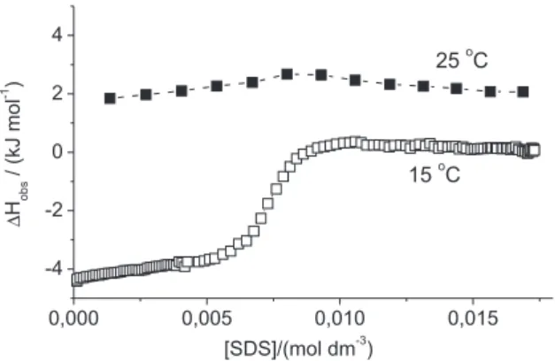
Here we have assumed that ∆Hdemic differs from zero. However, ∆Hdemic varies strongly with temperature so it may happen that it becomes zero or close to zero at the temperature of the measurement. Such is the case for sodium dodecylsulfate, SDS, at 25 °C where only a change of slope of ∆Hobs is observed at the expected c.m.c., see Figure 1. A change of temperature from 25 to 35 °C will change ∆Hmic from −0.2 to − 5.2 kJ mol-1 for SDS.11
Before discussing further how to calculate ∆Hmic as well as the c.m.c. we must define what we mean by the c.m.c. The concept of a critical micellization concentration is not well defined but has its most precise interpretation within the (pseudo)phase separation model. The definition of c.m.c. within the framework of other models is less clear.12,13
The book by Evans and Wennerström 13 is recommended for
study as it gives an authoritative but accessible discussion of various models for micelle formation.
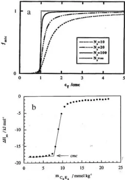
The plot in Figure 2a shows how the fraction fmic (= d {N[SN]}/dcT) that forms micelles varies with the total surfactant concentration, cT, when an incremental amount of amphiphile is added, for various values of the aggregation number N.14 The amphiphile concentration is
normalized to the c.m.c. The curve for N = ∞ represents the behavior at true phase separation. For N =100, the break is sharp and within a very small concentration range fmic will shift from 0 (= no micelles form) to 1 (= all added amphiphile gives micelles). For N = 20, the rise in fmic is still fairly steep but the bend in the curve is fairly wide and at twice the c.m.c. a significant fraction of added amphiphile stays as monomer. The smaller N is, the wider the range
Figure 1. Calorimetric titration curve from additions of 10 mass % SDS
where fmic has values between 0 and 1. For N = 10, fmic has still not reached 0.95 at five times the c.m.c., that is 5 % of added amphiphile dissolves as monomers.
Calorimetric titration curves obtained from consecutive additions of a small quantity of concentrated amphiphile solution starting with pure water and where the observed enthalpy change per injection, ∆Hobs, is plotted against total amphiphile concentration will reflect the shape of Figure 2a. This is exemplified by the calorimetric titration curve for 10 wt.% C8EO4 (n-octyl tetraoxyethylene glycol monoether) in water, shown in Figure 2b.15 If the change
in concentration in each titration step is reasonably small, the following is valid to a good approximation:
∆Hobs = (1− fmic) ∆Hdemic + ∆Hdil (7)
In the beginning all added micelles break up to monomers and fmic is zero. In the c.m.c. region a fraction (1 – fmic) will change into monomers while a fraction fmic will remain in micellar form. The steepness of the
titration curve (normalized to the c.m.c.) is an indication of the cooperativity of the aggregation process, i.e. of the aggregation number N. The curve for C8EO4 closely resembles the curve in Figure 2a for N = 20. In Figure 2a, the c.m.c. is defined as the concentration where 1% of surfactant is in micellar form. The concentration at the crossing point in Figure 2b between extrapolated initial and linear ascent lines will be close to the c.m.c. defined in this way. It will be the concentration where the start of formation of micelles is detected. However, the c.m.c can be defined and derived in other ways from calorimetric titration curves. The inflection point in the titration curve can be chosen as a measure of the c.m.c.16 This will be
close to the recommendation in reference 13 that “A good measure of this concentration (c.m.c.) is where an added monomer is as likely to enter a micelle as to remain in solution” that is at fmic = 0.5. The concentration at the intersection of the pre- and post-micellar tangents in the curve of the cumulative enthalpy changes, that is the integral enthalpies of dilution, has also been denoted the c.m.c.17We recommend that the c.m.c is determined as the
concentration at the inflection point in the calorimetric titration curves.
For large N, say above 50, and accordingly low c.m.c., values of c.m.c. defined in either way will be very close and the difference insignificant compared to experimental uncertainties. For such systems, the (pseudo) phase separation model usually suffices for a (basic) thermodynamic description. In this model the c.m.c is simply the saturation concentration of surfactant in monomer form.
However, for smaller N different ways to define the c.m.c. will give numerical values that differ significantly compared to experimental uncertainties. For C8EO4 as shown in Figure 2b, the difference will be of the order of 1 mmol kg-1, that is, significantly larger than the
experimental uncertainty. Thus, care should be taken when reporting to describe how values of c.m.c have been derived.
The variable fmic in Figure 2a was calculated from the mass action law model for micelle formation, also named the closed-association model in reference 13.
N S = SN KN =[SN]/[S]N (8)
This model gives a good description of basic features of micelle formation of nonionic amphiphiles such as C8EO4. In dilute solution of nonionic surfactants, the activities of the solute species can be approximated with concentrations. From fits of this model to calorimetric titration curves, values of c.m.c, ∆Hmic and aggregation number N can be
Figure 2. (a) The fraction fmic of incremental surfactant converted to
obtained.15,18 (The Nth order equation (8) can be solved using,
for instance, Newton Raphson’s numerical method.) The shape of the calorimetric titration curve will depend on the aggregation number N, the size distribution of the micelles and on the purity of the sample. The curves are S-shaped but, as Figure 2 shows, they do not need to be symmetric. This figure depicts micelle formation of a pure homologue of a nonionic amphiphile (C8EO4) with an aggregation number of just above 20. If the sample contains impurities of other homologues or other impurities this will influence the aggregation process and change the shape of the calorimetric titration curve. Triton-X100 has a low c.m.c., 0.27 mmol kg-1, but the micellization range
is large and does not reflect the large aggregation number (N > 100) due to the presence of homologues with varying ethylene oxide contents.15
Micelle formation of ionic surfactants is more complicated. It can be described as an equilibrium between charged surfactant ions S–, counterions B+ and micelles S
N:
N S– + (N – P)B+ = S N
–P (9)
KN = ([SN–P]/([S–]N [B+])N–P (10)
For large aggregation numbers, say above 50, and accordingly fairly low c.m.c., the titration curves will resemble fmic in Figure 2a, with a sharp rise at a certain concentration in the same way as for nonionic amphiphiles.
While the monomer concentration of nonionic amphiphiles above the c.m.c will be fairly constant, the monomer concentration for ionic amphiphiles decreases above the c.m.c. This is because the product [S−][B+]
remains constant above the c.m.c but as the concentration of unbound B+ increases with increasing total amphiphile
concentration, [S−] decreases, leading to an increase in
micelle concentration.19 The quantitative description of
the micelle formation process is difficult using the mass action law model.13 The most comprehensive treatment
has been made by Woolley and Burchfield20,21 in their
extensive study of the thermodynamic properties of alkyltrimethylammonium bromides. Archer has studied how values of ∆Hmic obtained from various models are influenced by various assumptions about, for instance, aggregation number, counterion binding and ion interaction parameters.22 His comparison illustrates that similar models
but slightly different assumptions can give large differences between derived values. A more direct method with fewer adjustable parameters is based on the treatment of the electrostatic interactions using the Poisson–Boltzmann equation.11,13,23-25
3.1.1. How to derive ∆Hmic
We start with nonionic amphiphiles. Relation (6) shows that if we extrapolate the (differential) dilution enthalpies below and above the c.m.c. to the c.m.c., the difference is:
∆Hobs(initial at c.m.c.) −
∆Hobs(final at c.m.c) = ∆Hdemic = − ∆Hmic (11)
This value is the enthalpy of formation of micelles at the c.m.c. from monomers at the same concentration. At the c.m.c., the concentration of micelles will be small so the (differential) dilution enthalpies just below and above the c.m.c. will be nearly the same. Note that ∆Hmic is independent of the titrant concentration. It should be kept in mind that ∆Hmic is a differential enthalpy change.
3.1.2. Pre-micellar region
Usually, the observed dilution enthalpies in the pre-micellar region are not constant but show an endothermic slope with increasing concentration. In the case of C8EO4 the slope was 80 dm3 kJ mol-2 and did not vary with
temperature in the range 10 to 40 °C.15 Charged amphiphile
ions show the same behavior. For SDS11 the slope in the
pre-micellar region was found to be 124 dm3 kJ mol-2 and
102 dm3 kJ mol-2 for lithium perfluorononanate26 and again
not varying with temperature. The slope increases with the length of alkyl chains and the increase in hydrophobicity. This nonideality in the pre-micellar region is ascribed to pairwise interaction between the hydrophobic chains.27,28
Usually, ∆Hobs varies linearly with concentration and the short extrapolation to the c.m.c. does not introduce any significant uncertainty in ∆Hmic.
As micelles cannot exist in an infinitely dilute solution it is not meaningful to attempt to derive a “standard ∆Hmic” by extrapolating the dilution enthalpies in the pre-micellar region to zero concentration.
3.1.3. Post-micellar region
For nonionic surfactants with large aggregation numbers, N > 50, and accordingly low c.m.c., ∆Hobs is expected not to vary significantly above the c.m.c. as there will be no further break up of micelles and, at a low total amphiphile concentration just above the c.m.c., dilution effects will be small. Extrapolation of ∆Hobs back to the c.m.c will not introduce any significant uncertainty. At concentrations well above the c.m.c. secondary changes such as micellar growth may take place that may give measurable enthalpy effects.
seen in the figure, there is a significant slope in ∆Hobs above the c.m.c. However, this slope is not due to dilution effects but to a continued break up of micelles. Still, at four times the c.m.c. a small but significant fraction of added micelles break up to monomers, cf. Figure 1 in reference15. In this case where the aggregation number is of the order of 25, routine extrapolation back to the c.m.c. of ∆Hobs from close to the c.m.c. will give an erroneous value of ∆Hmic.
∆Hobs should be measured well above the c.m.c. to find a region where the curve has become flatter. In this case, extrapolation back from concentrations above, say, five times the c.m.c will give a better value. In order to obtain a reliable value, the micelle formation process should be modeled using the mass-action law model to find out at what concentration demicellization can be ignored.
The c.m.c for ionic amphiphiles are much higher than for a corresponding nonionic surfactant. For example, the c.m.c for C12E8 is 7.1 × 10⁻⁵ mol dm-329 while it is 100 times higher
for SDS (8.3× 10⁻³ mol dm-3).30 Both surfactants have about
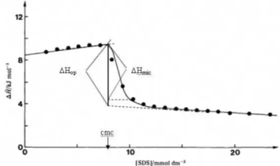
the same aggregation number at the c.m.c. of about 60. Due to the higher concentration and the presence of charged species, the dilution enthalpies in the post-micellar region may be significant and also vary noticeably with increasing concentration. For amphiphiles with large aggregation numbers (N > 50) micelle formation will be complete close to the c.m.c. but there will be an additional contribution to ∆Hobs in the post-micellar region from the decrease in monomer concentration, that is, the additional formation of micelles that takes place above the c.m.c. Usually ∆Hobs in the post-micellar region shows a more or less pronounced slope with increasing concentration. Extrapolation of a linear section back to the c.m.c will give a value of an operational ∆Hmic that may include a significant contribution from post c.m.c. aggregation. The problem is illustrated in Figure 3 which shows the situation for SDS in water at 35 °C. The curve is based on results of titration calorimetric measurements of consecutive additions of 28 mass % SDS solution starting with pure water in the cell.11 In this figure, c.m.c. is defined
as the concentration where 1% of SDS is in the form of micelles. Extrapolation to the c.m.c of the pre-micellar line and the post-micellar line starting at about 12 mmol dm-3
gives ∆H(op) = –6.0 kJ mol-1. However, calculation of
concentrations of SDS in monomer and micellar form using the thermodynamic model proposed by Jönsson and Wennerström23-25 with the electrostatic interactions
treated using a Poisson-Boltzmann approach shows that the slope above 12 mmol dm-3 to a large extent arises from
continued micelle formation. At the concentration where no micelles are formed or broken c(α=0), which is at about 9.5 mmol dm-3, added SDS micelles will only be diluted.
The difference between the observed dilution enthalpy at this concentration, ∆H(obs) (final at c(α=0)), and the initial dilution enthalpy extrapolated to the c.m.c., ∆Hobs(initial at c.m.c.), will give the correct value for the enthalpy of micelle formation:
∆H(mic) = ∆H(obs) (final at c(α=0) − ∆Hobs(initial at c.m.c.)) (12)
The value of ∆H(mic) = − 5.1 kJ mol-1 is ca. 10% smaller
than ∆H(op).
(In case c.m.c is defined as the concentration at the inflection point, the difference between ∆H(op) and true
∆H(mic) will be about the same.)
Without a detailed analysis using a theoretical model based on the Poisson-Boltzmann equation or a more advanced treatment or an elaborated mass-action law model, it is not possible to evaluate the contribution from the additional micelle formation in the post-micellar region. Therefore, we must conclude that values of the enthalpy of micelle formation derived from extrapolation of post-micellar dilution enthalpies will give values of ∆H(op) that must be considered estimates of ∆H(mic). This discussion applies to micelle formation in pure water. In solutions with extra salt the variation of ∆Hobs with amphiphile concentration is much smaller as the presence of extra electrolyte will reduce dilution effects and suppress the decrease in monomer concentration. While titration curves from dilution of a micellar solution of SDS in pure water show significant slopes above the c.m.c., values of ∆Hobs become constant close to the c.m.c in 0.1 mol dm-3 NaCl
solution.15 (The presence of extra salt also lowers the c.m.c
and changes ∆Hmic.)
For ionic amphiphiles with low aggregation numbers, say N of 10 to 15 or lower, it will not be possible to derive reliable estimates of ∆Hmic directly from the titration
Figure 3. Comparison between experimental (points) and calculated
(full line) titration curves for addition of 28 mass % SDS into water at 35 oC, indicating the difference between the true (∆H
mic) and operational
curves.31 At the c.m.c. the demicellization reaction is not
complete but will continue well above the c.m.c and it is not possible to determine where demicellization ends, cf. Figure 2. The micelle formation process needs to be modeled using a model based on the Poisson-Boltzmann equation or a mass-action law model in order to allow the determination of a reasonable value of ∆Hmic. The addition of extra salt will promote the aggregation and reduce dilution effects but it will change the aggregation properties from those in water.
It is also necessary to consider the concentration of monomers in the titrant solution. If ∆Hmic is calculated from the total concentration of surfactant and a significant fraction of the surfactant is in the form of monomers, the value will be in error. From what was said above, it is clear that it is not straightforward to calculate the monomer concentration, particularly not for ionic amphiphiles. In 0.08 mol dm-3
SDS, that is 10 times the c.m.c., the monomer concentration is still of the order of 0.004 mol dm-3, that is, about 5%
of SDS is in monomer form.32 Neglect of the presence of
monomers will give an error of 5% in the derived value of
∆Hmic. If instead the monomer concentration is assumed to equal the c.m.c, the error will be about 10%. Thus, it is necessary to use a high concentration of surfactant in the titrant solution, above 20 times the c.m.c, in order to derive reliable values of ∆Hmic,unless the monomer concentration is calculated and corrected for.
In summary, enhalpies of micelle formation, ∆Hmic, can be derived from calorimetric titration curves of consecutive additions of small amounts of micellar solution. The observed differential enthalpy changes before and after the c.m.c are extrapolated to the c.m.c and the difference equals ∆Hmic, provided the aggregation number is large, say above 50. This will give reliable ∆Hmic values for nonionic amphiphiles. For ionic amphiphiles values of ∆Hmic derived in this way may contain contributions from additional formation of micelles above the c.m.c.
For amphiphiles with lower aggregation numbers, extrapolation of ∆Hobs from just above the c.m.c. back to c.m.c. can give erroneous values of ∆Hmic due to an incomplete aggregation reaction. In the case of nonionic amphiphiles the aggregation can be modeled with sufficient accuracy by the mass action law model assuming a constant aggregation number N and approximating activities with concentrations. For ionic amphiphiles the change in monomer concentration above the c.m.c needs to be modeled using a mass action law model or a Poisson-Boltzmann approach. When reporting results, it is important to describe how values of c.m.c. and ∆Hmic were derived. When using values from the literature it is important to find out what they represent, that is, how they were derived.
3.2. Surfactants and polymers
Systems containing surfactants and water-soluble polymers are of great interest both for their widespread applications and for their inherently interesting properties. Such systems have long been subject to intensive research and an introduction to and overview of the field can be found in references 33 and 34. The use of titration calorimetry is more recent but as commercial titration microcalorimeters are now available, the method has become more attractive for studies of surfactant-polymer systems. In the following, we will discuss some practical considerations when using titration calorimetry to study such systems. We will start to discuss systems containing nonionic water-soluble polymers, first linear homopolymers, then hydrophobically modified polymers, followed by self-aggregating block copolymers. Then we will discuss studies of surfactant interaction with charged polymers, that is, with polyelectrolytes.
3.2.1. Surfactants and homopolymers
The most studied surfactant–polymer system is SDS and poly(ethylene oxide), PEO, and that applies also to calorimetry.35-38 When SDS is added to a PEO solution,
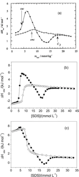
the self-association of SDS is facilitated by the presence of the polymer and cooperative aggregation starts at a critical aggregation concentration, c.a.c, that is lower than the c.m.c. A typical titration curve from addition of concentrated (10 mass %) SDS to a dilute PEO solution at 25 °C is shown in Figure 4a. The molar mass of PEO was 1.5× 10⁶ g mol-1 and the
concentration 0.23 mol repeat unit kg-1 (0.1 mass %). At this
temperature ∆Hmic (at c.m.c.) of SDS is small (− 0.2 kJ mol-1)
so the dilution curve in water shows only a change of slope at the c.m.c. Differences between the titration curve in the polymer solution and the dilution curve in water are dominated by SDS-PEO interactions. The slope of the curve in the PEO solution starts to deviate from the dilution curve in water above 3.5 mmol kg-1 SDS to give a pronounced endothermic
peak followed by a broad and shallow exothermic one. Then the curve joins the dilution curve at about 20 mmol kg-1. The
onset of aggregation of surfactant in the presence of polymer is characterized by a critical aggregation concentration, c.a.c. As for c.m.c. there is no generally agreed way to evaluate c.a.c. It can be defined as the concentration at the start of the endothermic peak and can be determined as the concentration at the crossing point between the extrapolated dilution curve and the linear ascent of the peak.36-38 This definition of the c.a.c.
surfactant to polymer solution vary with temperature and the system studied and the concentration where the titration curve in polymer solution starts to deviate from the dilution curve in the same solvent is the most practical choice, see Figures 4b and 4c. Figure 4b shows a titration curve of SDS in PEO solution at 15 °C and 4c the results of titrations at 35 °C.37
At 15 °C ∆Hmic is 4.8 kJ mol-1 and at 35 it is − 5.4 kJ mol-1.
The initial endothermic peak has decreased at 35 °C and has completely vanished at 45 °C.37 At the same time the
subsequent shallow exothermic peak disappears and the curve in the polymer solution will join the dilution curve in water from the endothermic side. At a second critical concentration, denoted c2, the influence of the polymer on the aggregation of surfactant in the calorimeter cell ceases, the free monomer concentration reaches the c.m.c and free micelles start to form. We define c2 as the concentration where the titration curve in polymer solution joins the dilution curve in water. The value of c2 increases in proportion to increasing polymer content. It is a less well-defined concentration and derived values will be quite uncertain. The pronounced features of the titration curve show that the interaction between SDS and PEO is complex and goes through different stages. Similarly shaped titration curves have been observed for other polymer–SDS systems39,40 and for sodium dodecylbenzenesulfonate and
poly(vinylpyrrolidone) (PVP)41 at ambient temperatures, where
∆Hmic of the surfactant is close to zero. The shape of the titration curves will change considerably if the temperature changes because both ∆Hmic and surfactant–polymer interactions vary strongly with temperature.36,37,39,41 However, it is still possible
to estimate values for the c.a.c. and c2 as the concentration where the curve in the polymer solution starts to deviate from the curve in water and where the two curves join again. The value of c.a.c. is important because it indicates the free energy change for surfactant-polymer interactions. The decrease in free energy for surfactant aggregation in the presence of polymer can be estimated from: ∆∆Gagg = RT ln(c.a.c./c.m.c.). For “true” polymers, as in the case of PEO with molar masses aboveabout4000 g mol-1, the value of c.a.c. is independent of
polymer chain length and concentration.36,37,42-44
Before we continue the discussion we will look in more detail at the events when SDS is added to PEO in solution in order to get a better description of the titration curves. We will refer to experiments giving the curves shown in Figure 4. The concentration of the SDS solution in the syringe was 10 mass % so the monomer concentration is negligible and the PEO concentration was 0.1 mass %. In the first few injections, that give final concentrations below the c.a.c., the processes will be the same as described by equations (1) to (3). However, the observed differential enthalpies of dilution ∆Hdil(ci) differ somewhat from those in pure water. The difference indicates a weak endothermic
interaction between SDS monomers and polymer chains. When the total surfactant concentration increases to above the c.a.c., the added micelles will break up to monomers and a fraction β will aggregate on the polymer while the fraction (1−β) stays in non-aggregated form in solution:
N SN(C0) + P(ck-1) = (1− β) S(ck) + β (M SMP(ck)) (13)
∆H(13) = ∆Hdil(ck) + (1− β) ∆Hdemic + β∆HaggM
Here S(ck) denotes monomeric amphiphile of concentration ck and SMP(ck) is the amphiphile in the aggregated form of the concentration after the kth injection,
M is the aggregation number of polymer-bound aggregates
Figure 4. Calorimetric titration curves from addition of 10 mass %
SDS to 0.1 mass % PEO (solid circles), at: (a) PEO 1.5 x 10⁶ g mol-1, at
25 oC (adapted from ref. 34), (b) 15 oC and (c) 35 oC, both for PEO 3350
formed at this concentration and P indicates polymer. The aggregation number M will increase with increasing total concentration and the monomer concentration also increases. Above c2, the free monomer concentration has reached the c.m.c and the added micellar solution will only be diluted, see equation (4). The observed enthalpy change will be ∆Hdil(cf) at the final concentration cf.
In order to evaluate the (differential) enthalpy change for aggregate formation, ∆HaggM,we must be able to evaluate the extent of binding,β, which means that we must know the binding isotherm. The determination of binding isotherms is more cumbersome than the calorimetric experiments and, therefore, they are usually not known. When ∆Hdemic is close to zero, as in Figure 4a, the difference between the titration curve in polymer solution and the dilution curve in water at a certain SDS concentration indicates the enthalpy of formation of polymer-bound aggregates at that total concentration. But, as the amount of aggregates formed is not known, we cannot calculate the (differential) molar enthalpy change ∆HaggM. However, the features of the curves give qualitative information about the progress of aggregation with increasing concentration.39,41
In case the binding isotherm has been determined, the differential enthalpy of aggregation, ∆Hagg, can be calculated as a function of amphiphile concentration. We can elaborate equation (13) to indicate the process during the kth injection of ninj mol of S in micellar solution with
concentration Co:
ninj S
N(Co) + nk-1 Smon(ck-1) + nk-1 SM P(ck-1) →
nk Smon(ck) + nk SM P(ck) (13a)
The amount of S in monomeric and bound form, respectively, before injection is denoted nk-1 and after injection is nk. The observed enthalpy change qobsconsists of enthalpies of demicellization, dilution and aggregation. The fraction β of added surfactant that binds to the polymer is:
β = {nk SM P(ck) − nk-1 SM P(ck-1)}/ ninj (14)
The concentration of polymer-bound surfactant before and after injection can be calculated from the binding isotherm.
Now we inject the same amount of micellar S in a solution that already contains monomeric S at a concentration ci so that after the injection the monomer concentration is ck-1:
ninj S
N(C0) + Smon (ci) → n inj S
mon(c k-1) (15)
The observed enthalpy is qdemic +dil . Equation (13a) minus (15) gives:
(ninj + n
k-1 )Smon(c k-1) + nk-1 SM .P(c
k-1) →
nk Smon(ck) + nk SM.P(c
k) (16)
Values of β for the various injections are calculated from the binding isotherm and the differential aggregation enthalpies calculated from
∆Hagg =(qobs − qdemic +dil )/ β ninj (17)
The value of ∆Hagg for the kth injection relates to the
total amphiphile concentration S(ctot) = [Smon(ck) + SM P(ck)]. The correction for demicellization and dilution of the concentrated micellar solution is determined from dilution experiments where the final concentration of surfactant equals the monomer concentration in the binding experiment.40 The variation of the enthalpy of dilution of the
monomeric surfactant with concentration is assumed to be small. The dilution of the polymer solution is assumed to be negligible (This can be checked by blank experiments injecting solvent into polymer solution). ∆Hagg derived in this way is the differential enthalpy change for the formation of one mole of aggregate from monomers at the conditions of the kth injection:
Smon(ck) = M SMP(ck) (18)
This enthalpy change is also called binding enthalpy. At the second critical concentration c2, the formation of polymer-bound aggregates is complete and they coexist with monomers of concentration equal to the c.m.c. The integral (total) enthalpy change for aggregate formation
∆Hagg(int) can be estimated without use of binding isotherm as follows. Assume that c2 has been reached after Y injections of ninj S
N(Co) to give a total volume VY. At c2 the
monomer concentration equals c.m.c. Then,
∆Hagg(int) = [Σ qobs – Yqdemic +dil / (Y.ninj − V
Y(c.m.c.))]
(19)
where Σ qobs is thesum of observed enthalpies of the Y injections, qdemic +dil is the combined demicellization and dilution correction measured below the c.m.c., cf. equation (15). ∆Hagg(int) is the enthalpy change for the formation of one mole of aggregated surfactant from monomers over the concentration range from c.a.c. up to c2 (saturation).
The differential enthalpies of formation of aggregates of SDS and ethyl(hydroxyethyl)cellulose (EHEC) vary strongly with the SDS concentration which shows that the character of the SDS aggregates changes as the SDS concentration increases.40 At ambient temperatures, the
changes while the formation enthalpies become exothermic at higher SDS concentrations. Titration curves of SDS into dilute solutions of other uncharged polymers such as PEO and PVP show the same qualitative features.35
Titration calorimetric studies of polymer–surfactant interactions have been made where the titrant solution, in addition to the surfactant, contained polymer of the same concentration as the starting concentration in the calorimetric cell.45 This is made to avoid dilution of
the polymer solution during titration. If the surfactant concentration in the titrant solution is S(Co) and the polymer content P(wt) the mixed titrant solution can be described as [(1−X) N SN(Co) + X M SMP(wt)] where a fraction X of the surfactant is bound to the (saturated) polymer. Dilution in water of the mixed titrant solution will give:
(1−X) N SN(co) + X M SM P(wt) + solvent = Smon + P(wt) (20)
The observed enthalpy change will contain contributions from both dilution–demicellization and from the break-up of polymer-bound aggregates. The amount of S bound to the polymer may be significant. For instance, in a solution containing 0.1 mol dm-3 SDS and 0.1 mass % PEO the
concentration of unbound SDS will be about 0.09 mol dm-3
and of bound SDS 0.01 mol dm-3.46 As the enthalpy of
aggregation usually is not known, it is difficult to extract quantitative information from the results. Provided that the enthalpy of formation of the surfactant aggregates at c2 is close to ∆Hmic it will be possible to estimate values of c.a.c. and c2.
While anionic surfactants such as SDS interact strongly with neutral synthetic polymers such as poly(vinylalcohol), PVA, PEO, poly(propylene oxide), PPO and PVP, cationic surfactants interact only weakly or not at all.33,34,46,47 The
reason for this difference between anionic and cationic surfactants is not clear.
The interaction between nonionic surfactants and polymers of this type is usually very weak or nonexistent.34
Brackman et al.48 were the first to observe that there can be a
significant response in titration-calorimetric measurements from polymer–surfactant interaction although the decrease in c.m.c. is small. The titration curve from addition of concentrated solution of n-octyl β-D-thioglucopyranoside, OTG, to PPO solution differs significantly from the dilution curve in water but the bend in the curve indicating the change from demicellizaion to aggregation is not shifted much. The authors concluded that the c.m.c. was not significantly lowered. However, the titration curve in polymer solution is shifted about 1 mmol dm-3 to lower
concentrations, which shows that the aggregation of OTG
is influenced by the presence of the polymer and starts at a lower concentration. The double peaks reported by Brackman et al.48 probably are an artifact due to inefficient
stirring, as they were not observed by Wang and Olofsson using a different calorimeter with good stirring (see chapter 8 of reference 48). But the titration curves also reveal that there is significant interaction between PPO and OTG at higher concentrations. This indicates that the polymer interacts preferably with micelles of OTG. The nonionic surfactant C12E8 interacts in the form of micelles with ethylhydroxyethyl cellulose in aqueous solution49 and other
nonionic surfactants can be expected to interact in the same way as pseudo-polymers. We believe that if the polymer influences the aggregation of a surfactant that will lead to a lowering of the aggregation concentration c.a.c. However, the interaction may arise between surfactant micelles and the polymer and that may have only a minor effect, if any, on the c.a.c. values.
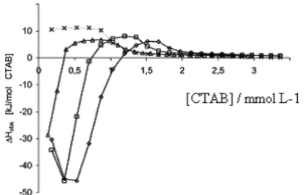
A d i f f e r e n t k i n d o f p o l y m e r – s u r f a c t a n t interaction was observed in a calorimetric study of hexadecyltrimethylammonium bromide, CTAB, and starch polysaccharides.50 The shape of the titration curves differed
from the curves observed for the linear homologues discussed above. Figure 5 shows an enthalpic titration curve from addition of 0.022 mol dm-3 CTAB to solutions of amylose from
potato at 27 °C. The curve for dilution in water is included. Binding isotherms were determined from careful surface tension measurements.51 The interaction is strong as shown
by low c.a.c. and gave strongly exothermic binding enthalpies that amounted to − 60 kJ (mol CTAB)-1. This is more than six
times the value for enthalpy of micelle formation of CTAB, − 9.5 kJ mol-1. In the amylase-CTAB inclusion complex the
polysaccharide winds around the alkyl chain of CTAB52,53 and,
thus, there is no self-aggregation of the surfactant.
The various reported studies of surfactants and polymers show that titration calorimetry gives useful information.
Figure 5. Calorimetric titration curve from addition of 22.0 mmol L-1
However, the final remark in reference 40 is worth to bear in mind: “Finally, we would like to emphasize the utility of combining measurements of varying techniques and more important the need for good binding data, to the study of such systems.”
When performing calorimetric measurements, it is important to keep in mind that in a calorimetric experiment of, say, addition of surfactant to a polymer solution, the total heat effect caused by this addition will be measured. This means that if side reactions such as ionization or protonation occur, this enthalpy effect will be included. Therefore, it is necessary to keep track of changes in pH when amphiphiles or polymers with ionizable groups such as weak acids or bases are used. The enthalpy changes can be large. For instance the protonation of a primary amino group will give an enthalpy change of the order of −50 kJ mol-1 in water at 25 °C.54 Poly(ethylene imine),
PEI, has primary, secondary as well as tertiary amino groups that can take up protons in aqueous solution. In the study by Winnik et al.55 of the SDS-PEI system using
various experimental methods, the pH was monitored and the extent of protonation found too small to give any significant enthalpy contribution. In that article the authors also review and discuss a number of earlier calorimetric studies of polymer-surfactant interactions.
3.2.2. Surfactants and hydrophobically modified uncharged polymers
Hydrophobically modified water-soluble polymers, HM-polymers, are polymers with hydrophobic groups chemically attached to a hydrophilic polymer backbone. The hydrophobic groups can be attached at the ends of the polymer backbone or the groups can be grafted along the polymer chain. Aqueous HM-polymers are capable of spontaneous aggregation through association of their hydrophobic moieties. The self-aggregation strongly increases the viscosity compared to the unmodified polymer. The self-association can be studied calorimetrically by performing measurements of dilution of concentrated polymer solutions in the same way as studies of micelle formation of surfactants, see section A.
Calorimetric titration curves from addition of surfactant to dilute HM-polymer solution will differ from curves observed for systems discussed in the previous section. Figure 6 shows titration curves from addition of SDS to 0.25 mass % solution of HM-EHEC and parent EHEC and of dilution in water.56 The degree of nonylphenyl
substitution was 1.7%, corresponding to ca. 6.5 groups per molecule. The binding of surfactant started at a much lower concentration than for the parent polymer and was seen as an endothermic displacement of the observed enthalpy.
When the SDS concentration exceeds the c.a.c., SDS will start to aggregate on the polymer in a way similar to the unmodified polymer. The effect of the hydrophobic groups is only evident at low SDS concentrations where SDS monomers solubilize in aggregates consisting of the grafted hydrophobic groups. However, as the SDS concentration increases, the HM-aggregates will become charged and disintegrate due to electrostatic repulsion between the DS− ions and the influence of the hydrophobic groups will
fade away as their concentration is low. Above the c.a.c. the binding of DS− ions becomes more cooperative and
resembles aggregation in the unmodified EHEC. Titration curves from addition of SDS to hydrophobically end-capped poly(ethylene oxide)dodecyl ether, C12EO200C12, and the parent PEO showed the same essential features, Figure 7 in reference 57. The addition of the cationic surfactant dodecyltrimethylammonium bromide, DTAB, to the C12EO200C12 polymer solution gave a different titration curve, see Figure 7 in reference 57. The first few injections gave significantly more endothermic enthalpy changes than the dilution in water. The differences decreased with increasing DTAB concentration, and were small at concentrations above the c.m.c. The results indicate that DTAB added in the beginning was solubilized in the C12 end-group aggregates that probably disintegrated, but showed no evidence of interaction between the surfactant and the PEO backbone at higher DTAB concentrations in accordance with expectation. This behavior will be observed when the main chain of the HM-polymer is so hydrophilic that it cannot induce aggregation of the surfactant. Titration curves from addition of surfactants to HM-polymer solutions can give interesting information about interactions in the systems. When performing experiments on HM-polymer-surfactant systems one should keep in mind that there may be large changes in viscosity that can have a strong influence on the stirring. Bench experiments with transparent cups will show if mixing is satisfactory. If this cannot be made, experiments with varying stirring speed are necessary. As in all studies of complex systems, calorimetric results must be combined with results from other types of experiments in order to gain an understanding of the system.
3.2.3. Surfactants and block copolymers
form micelles above the c.m.c. A notable feature of the self-association process is that a small temperature increase at the critical micellar temperature, c.m.t., can give a dramatic decrease in c.m.c. The self-association arises from the limited and temperature dependent solubility of the PO-block that gives aggregates with an essentially water-free hydrophobic core surrounded by more hydrophilic EO blocks. The copolymers are used in a wide range of applications and often together with surfactants. Therefore, block copolymer-surfactant systems have been studied using a variety of methods including ITC and DSC (differential scanning calorimetry). To our knowledge the first report of the use of ITC is the study by Li et al.59 of the
binding of SDS to EO97-PO69-EO97 where calorimetry was used in addition to EMF and light scattering. Later studies have been carried out on the interaction between typical triblock copolymers and cationic and nonionic surfactants in addition to SDS, seereferences 60 to 64.
Titration calorimetry is a useful and reasonably fast method to explore ranges of concentrations of interest. Many processes and events that take place in the systems as the composition changes will have measurable enthalpy changes and, thus, be seen in titration curves. Such curves determined at various temperatures can give a map of the system and locate concentration ranges where processes take place. These concentrations can now be studied by other methods to determine the nature of the processes and transitions. Figure 7 shows the titration curve from addition of 10 mass % SDS to 1.00 mass % solution of P123 (EO20-PO68-EO20) at 40 °C.63 The curve for dilution of SDS
in water is included. Comparison with Figure 4 shows that, in the copolymer system, the reaction between SDS and the copolymer gives a titration curve with totally different features. Static and dynamic light scattering results indicate that the large, broad exothermic peak reflects rehydration of
the PO blocks of the copolymer chains as the P123 micelle break-up upon surfactant addition.63
In addition to give information about enthalpy changes for a process, titration calorimetry can also give kinetic information. In a study of the system C12EO6-P123 in water at 40 °C, where small portions of concentrated surfactant solution were added to dilute P123, the time to reach equilibrium suddenly increased over a narrow concentration range to 15 to 20 min from a couple of minutes, see Figure 8. The event giving the slow reaction was confirmed by light scattering to be a sphere-to-rod transition of the mixed micelles. No attempt was made to derive quantitative kinetic information from the calorimetric curves.
The block copolymers appear as unimers in solution at temperatures below the c.m.t. The ionic surfactant SDS interacts almost independently at 15 °C with the PO and EO blocks in EO-PO-EO copolymers and show a c.a.c. value ascribed to the PO block that is closely the same as for PPO 2000, about 0.8 mmol dm-3. The calorimetric titration curve
from addition of a concentrated SDS solution to a dilute solution of EO52-PO35-EO52 shows similar features as the titration curve of a mixture of PEO 2000 and PPO 2000.65
3.3. Surfactants and polyelectrolytes: complex formation
Macromolecules carrying ionic groups that dissociate in water (or another ionizing solvent) to give multiply charged polyions and ions of opposite charge are called polyelectrolytes. Systems containing polyelectrolytes and surfactants are common and of great practical as well as scientific interest. Conditions for titration calorimetric studies of interactions between polyelectrolytes and
Figure 6. Calorimetric titration curves at 25 °C from additions of
10 mass % SDS to () 0.25 mass % ethylhydroxyethylcellulose (EHEC), () 0.25 mass % hydrophobically-modified EHEC and -- water. (reprinted, with permission from the American Chemical Society, from ref. 56).
Figure 7. Calorimetric titration curves from addition of 10 mass % SDS
nonionic surfactants will resemble studies of ionic surfactants and nonionic polymers as discussed above.66
As pointed out previously, independent determination of binding isotherms is required in order to make full use of calorimetric results.
Oppositely charged polyelectrolytes are particularly efficient in lowering the aggregation concentration of ionic surfactants, the critical aggregation concentration c.a.c. being usually a factor 100 to 1000 smaller than the c.m.c in pure water. But additions of an aqueous solution of an ionic surfactant to a solution of an oppositely charged polymer generally results in a phase separation due to the low solubility of the complex salt formed by the surfactant ions and the polyion. At increased surfactant concentrations the precipitate may “dissolve”.67 Thus, during a titration
experiment where surfactant solution is added to a dilute solution of oppositely charged polyelectrolyte (or vice versa) a precipitate may form that may dissolve as more surfactant
is added. The formation of the precipitate and its dissolution will have enthalpic effects. Therefore, before measurements are made on a new system with an unknown phase behavior, it is necessary to find out if precipitation will take place under the conditions of the intended calorimetric titration experiments. Prominent features in titration curves in such a system that appear at concentrations where precipitates form and disappear can then be ascribed to these events. As the system studied is complex, the resulting titration curve can be expected to be complex and difficult to evaluate, as can be seen in Figure 9, taken from reference 68. The article by Skerjanc et al.69 that reports enthalpy of binding of dodecyl-
and cetylpyridinium cations to poly(styrenesulfonate) anion is to our knowledge the first calorimetric study of polyelectrolyte–surfactant interaction. The binding isotherms were determined using surfactant-ion-selective solid-state electrodes. The article reports the kind of information that can be gained from such a study. For instance, they found that although the two surfactants started to bind at the same concentration, 10-5 mol dm-3, the degree of binding for the C
12
-salt ranged from 70 to 99% depending on surfactant and -salt concentration, while the C16-salt was almost quantitatively bound to the polyelectrolyte. The observed enthalpy changes (expressed per mole of surfactant) were constant between the start of binding up to charge neutralization (and start of phase separation). Quantitative evaluation of enthalpies of binding could be made as the binding isotherms were known. The enthalpies of binding were of the same order of magnitude as the enthalpies of micelle formation for the studied surfactants.
The determination of binding isotherms for polymer-surfactant systems is usually more cumbersome than
Figure 8. (A) Calorimetric titration curves for the addition of 10 mass
% C12EO6 to: () 1.0 mass % P123 solution and to () water, at 40 oC.
(B) ITC raw data for the same experiment, showing that some composite peaks with a fast endothermic process followed by a slower exothermic one (inset shows in more details the peaks indicated by the arrow). Adapted from reference 64.
Figure 9. Calorimetric titration curves for the addition of 0.2 mol dm-3
calorimetric measurements as no generally applicable experimental method with commercial equipment is available. Therefore, it is tempting to try to estimate the binding properties from titration calorimetric measurements by fitting observed enthalpy curves to a model isotherm. Lapitsky et al.70 report such an attempt to determine
isotherms for the systems sodium perfluorononanate-hydroxyethyl cellulose and dodecyltrimethylammonium bromide–sodium polystyrenesulfonate. Their model is based on the Satake–Yang adsorption model.71 The success
is limited and the authors discuss the limitations of the method. Their results show that this polymer-centered adsorption model is insufficient for the evaluation of quantitative binding isotherms from calorimetric titrations on polyelectrolyte-surfactant systems. Starting from a surfactant-centered viewpoint may be more fruitful but neither can a simple closed association (mass action law) model give quantitative predictions of binding isotherms (see chapter 5 from reference 34). More advanced models are needed to describe polymer-surfactant complexation. In our opinion it is not possible, except in very special circumstances, to determine binding isotherms from calorimetric titration curves. For the time being, independent experimental determinations are necessary.
4. Concluding Remarks
In titration calorimetry usually small portions of a concentrated solution of surfactant R2 (or pure R2) are added successively to a solution of reactant R1 or pure solvent at the start of titration in the calorimeter vessel and the enthalpy change qi is measured. The concentration of R2 increases for each addition and qi results from the processes that occur in the titration steps. Thus, the measured enthalpy changes are differential enthalpies that, for small concentration changes, approximate partial molar enthalpies. Very useful qualitative information can be obtained from calorimetric titration experiments as calorimetric titration curves can show that events take place and the concentration where they occur. In this way large concentration ranges can be mapped in a limited length of time. This is very useful when designing experiments by other methods that can probe the molecular nature of the processes.
In order to derive quantitative information about aggregation enthalpies, the processes that take place in the titration steps must be identified. In experiments were binding to, for instance, polymers occurs, the knowledge of the binding isotherm is necessary.
Modern commercial titration calorimeters are sensitive so measurements can be made at concentrations that are below the range of other methods.
Acknowledgments
W.L. thanks the Brazilian Agencies FAPESP and CNPq for support to the various research projects whose results are cited in this review and FAPESP for supporting visits between Lund and Campinas. The authors would also like to thank co-workers who participated in the cited studies and whose names are cited in the references.
Gerd Olofsson was born in 1936 and got her bachelor and licenciate degrees at Uppsala University, Sweden, followed by the doctor’s degree in chemistry at Lund University in 1968. Since 1976 she has been Senior Lecturer in Chemistry at Lund University. Her research interest has been thermochemical - thermodynamic characterization using mainly various reaction-solution calorimetric methods starting with donor - acceptor interaction between antimony pentachloride and molecules containing carbonyl groups. The major part of her research work deals with aggregation and adsorption of surfactants in solution. Present research interests are thermodynamic characterization of interactions between ionic amphiphiles and polymers (charged or uncharged) in aqueous solution. She has been actively involved in the work of the International Union of Pure and Applied Chemistry, IUPAC, and has been secretary of IUPAC Commission I.2 on Thermodynamics 1987 – 1993, and secretary of the Physical Chemistry Division Committee 1995 – 2001.