Agrometeorology |
Article
index in the State of São Paulo, Brazil: trends and
spectral features under the normality assumption
Gabriel Constantino Blain (*)Instituto Agronômico (IAC), Centro de Pesquisa e Desenvolvimento de Ecofisiologia e Biofísica, Caixa Postal 28, 13012-970 Campinas (SP), Brazil.
(*) Corresponding author: [email protected]
Received: April 5, 2011; Accepted: Sept. 5, 2011
Abstract
The aim of this study was to describe monthly series of the Standardized Precipitation Index obtained from four weather stations of the State of São Paulo, Brazil. The analyses were carried out by evaluating the normality assumption of the SPI distributions, the spectral features of these series and, the presence of climatic trends in these datasets. It was observed that the Pearson type III distribution was better than the gamma 2-parameter distribution in providing monthly SPI series closer to the normality assumption inherent to the use of this standardized index. The spectral analyses carried out in the time-frequency domain did not allow us to establish a dominant mode in the analyzed series. In general, the Mann-Kendall and the
Pettitt tests indicated the presence of no significant trend in the SPI series. However, both trend tests have indicated that
the temporal variability of this index, observed at the months of October over the last 60 years, cannot be seen as the result of a purely random process. This last inference is due to the concentration of decreasing trends, with a common beginning (1983/84) in the four locations of the study.
Key words: Pearson type III distribution, drought, climate trends.
Valores mensais do índice padronizado de precipitação pluvial no Estado de São Paulo,
Brasil: tendência e características espectrais sob o pressuposto da normalidade
Resumo
O objetivo do trabalho foi descrever séries mensais do Índice Padronizado de Precipitação (SPI), obtidas a partir de quatro es-tações meteorológicas do Estado de São Paulo, Brasil (1951-2010). As análises foram realizadas avaliando-se o pressuposto de normalidade das distribuições do SPI, as características espectrais dessas séries e a presença de tendências climáticas nessas amostras. Observou-se que a distribuição Pearson tipo III foi melhor que a gama 2-parâmetros em prover séries men-sais do SPI mais próximas ao pressuposto de normalidade inerente ao uso desse índice padronizado. As análises espectrais realizadas no domínio tempo-frequência não permitiram o estabelecimento de modo (de frequência) dominante nas séries
analisadas. De forma geral, os testes de Mann-Kendall e Pettitt não indicaram a presença de significativas tendências nas séries do SPI. Entretanto, verificou-se que a variabilidade temporal desse índice, observada em outubro, não pode ser vista
como o resultado de um processo puramente aleatório. Essa última inferência é devida à concentração de tendências de queda, com data inicial comum (1983/1984), nas quatro localidades do estudo.
Palavras-chave: Pearson tipo III, seca, tendências climáticas.
1. INTRODUCTION
Strongly related to a deficit in the rainfall amounts, the drought events can cause severe damages to human so-ciety. Under this consideration, the standardized pre-cipitation index (SPI) was developed by McKee et al. (1993) as a statistical procedure (normalized in time--space domain) capable of representing drought and flood events in a similar probabilistic way, even when different rainfall regimes (observed in distinct regions and periods) are being evaluated (Wu et al., 2007). Also
according to Wu et al. (2007), being normally distribu-ted is the major reason that leads the SPI to be widely accepted in operational mode as well as in academic studies all over the world.
index to evaluate, on regional basis, the frequency, the duration and, the intensity of the drought events detec-ted in Greece from 1951 to 2000. Mishra et al. (2007) employed the SPI to evaluate, among other features, the transition probabilities of drought events in the Kansabati River basin; India. By using the SPI, Zhang et al. (2009) observed changes in the events of drought and wetness in Pearl River Basin; China (1960-2005). Zhai et al. (2010) demonstrated that the SPI can be used to describe possi-ble trends in the dryness and wetness severity in the re-gions of China, as well as in other countries. Manatsa et al. (2010) used the SPI to address several features of agri-cultural droughts in Zimbabwe, Africa. Li et al. (2008) observed that the values of the SPI computed over sou-thern Amazon region decreased in the period of 1970 to 1999 by 0.32 per decade. According to these authors this result indicates an increase trend in dryness conditions.
In Brazil, the SPI is largely used on operatio-nal mode by governmental agricultural institutions, such as Empresa Brasileira de Pesquisa Agropecuária (EMBRAPA; www.agritempo.gov.br), Instituto Agronômico (IAC; www.infoseca.sp.gov.br) and, Instituto Nacional de Meteorologia (INMET; www.inmet.gov.br), in order to monitoring (possible) drought conditions in diffe-rent regions of the country. Furthermore, the studies of Fernandes et al. (2010), Macedo et al. (2010) and, Sansigolo (2004), address the use of the SPI in the clima-te conditions of Brazil. In order to assess the robustness of the SPI (among other drought indexes) in estimating the upland rice yield (1983/1984 - 2005/2006; Goiâna- State of Goiás), Fernandes et al. (2010) have addressed important features (including its limitations) of the use of this standar-dized index as an agricultural drought indicator. Macedo et al. (2010) calculated the SPI in order to monitoring drought events within three rainfall homogeneous sub-regions of the State of Paraíba. The main purpose of Sansigolo (2004) was to establish a comparative performance analysis between the Palmer Drought Index (Palmer, 1965) and the SPI in Piracicaba, State of São Paulo.
However, despite all the concerns related to the possi-ble consequences of the global warming over the temporal variability of drought events, such as a possible increasing in its intensity and frequency, the evaluation of the presen-ce of trend components in time series of this drought index seems to be still neglected in the Brazilian literature. Thus, considering that the analysis of long SPI series provides im-portant information to the climate literature, which may be helpful in reducing the human vulnerability to drought events, the aim of the study was to describe the temporal variability of monthly SPI series obtained from four wea-ther stations of the State of São Paulo. This description was carried out by evaluating (i) the normality assumption of the SPI distributions, (ii) the spectral features of these se-ries (including their possible relationship with the ENOS) and, (iii) the presence of climate trends in these datasets.
2. MATERIAL AND METHODS
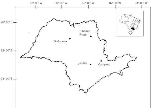
Monthly rainfall series available from four weather sta-tions of the State of São Paulo, Brazil (Campinas, 1890 to 2010; Jundiaí 1942 to 2010; Pindorama, 1951 to 2010 and; Ribeirão Preto 1937-2010; figure 1) were chosen for this study. After Guttman (1994) has investigated the effect of the length of the data records on rainfall distri-butions, he stated that at least 40-60 years are required for parameter estimation stability. Thus, the series were chosen in order to provide 60 years of data records. The selected series did not have missing values and their con-sistencies were assessed in Blain (2009). Also according to Blain (2009) the main feature of the monthly rainfall series (PRE) of the State of São Paulo is its great varia-bility in time-space domain. For a given location it can be observed strongly skewed rainfall distributions during the winter season; however, during the summer season the shape of these monthly distributions becomes similar to the “bell shape” of the Gaussian distribution.
The gamma 2-parameter distribution (Gam) is fre-quently used in the State of São Paulo (as well as in others regions of Brazil) in describing monthly rainfall recor-ds (and, therefore, in the SPI calculation algorithm). However, according to Guttman (1999) the Pearson type III (PE3) distribution, also known as gamma 3-pa-rameter, is ‘the best universal model for the SPI calcu-lations’. Furthermore, Wu et al. (2007) stated that the confidence in SPI results, obtained from the Gam distri-bution (undefined for the 0 value), can be affected since this probability density function has only two free para-meters. According to these authors, the use of alternatives distributions, such as the PE3, is worth to be evaluated. In this study, the cumulative probability associated with a given monthly rainfall amount [H(PRE)] was compu-ted from these two probabilistic models (Gam and PE3). The Gam model was estimated as described in Wu et al. (2005) and Wu et al. (2007), while the PE3 was estima-ted as recommended by Guttmann (1994, 1999) and Yue and Hashino (2007). In order to obtain the SPI, the [H(PRE)] values were subject to the standardization procedure based on the following equations proposed by Abramowitz and Stegun, (1965).
1 H(PRE) 0.5 when 1 0.5 H(PRE) 0 when 1 3 3 2 2 1 2 2 1 3 3 2 2 1 2 2 1 < < + + + + + + = < + + + + + = t d t d t d t c t c co t SPI t d t d t d t c t c co t SPI − − − ≤ (1) where = 2 )) ( ( 1 ln( PRE H t
when 0 < H(PRE) ≤ 0.5
= 2 )) ( 1 (
1 ln(
PRE H t
− when 0,5 < H(PRE) <1
c
o = 2,515517; c1 = 0,802853; c2 = 0,010328; d
1= 1,432788; d2 = 0,189269; d3 = 0,001308
Although the use of the Gam distribution in charac-terizing monthly rainfall series of the State of São Paulo has already been extensively evaluated (Blain et al., 2007; Blain et al., 2009; Blain 2009; 2010), the use of PE3 distribution for this purpose seems to be little assessed. Since the SPI is a probabilistic index, assessing the robus-tness of the PE3 distribution in describing rainfall series may be seen as the first step in the study of the possibility of adopting this distribution in the SPI calculations.
As discussed by Wilks (2006), Steinskog et al. (2007) and, Vlcek and Huth (2009), if (and only if) the para-meters of the theoretical distribution have not been esti-mated from the same dataset used to evaluate the fit of the parametric distribution, the original algorithm of the Kolmogorov-Smirnov test is applicable. Thus, since the three parameters of the PE3 were fitted using all available data, the test had to be modified. Hereafter this adapted method will be referred as Kolmogorov-Smirnov/Lilliefors test (KS-L). The statistical simulations required for calcu-lating the KS-L test were based on the procedure called “nonuniform random number generation by inversion”. It
were generated Ns=100000 synthetic data samples. More information about the KS-L can be found in Wilks (2006).
According to Edwards and Mckee (1997) and Wu et al. (2007) despite the presence of equations 1 and 2 within the SPI algorithm, for dry climates or those with a distinct dry season associated with strongly skewed rain-fall distributions (in which the zero value is common), the SPI series may not be normally distributed. At this point, it is worth emphasizing that also according to Wu et al. (2007) the SPI is widely accepted throughout the world because, conceptually, ‘it is normalized to a location and is normalized in time’. Thus, a normality test was applied on the SPI values obtained from the Gam and from the PE3 models. The parametric distribution capable of pro-viding the greatest number of normally distributed SPI series will be seen as the best probabilistic model for the calculations of this standardized index. The SPI series will be considered as coming from a standard normal distri-bution if at least one of the following criteria is met: (a) Shapiro-Wilks statistic (W) equal or greater than 0.96 (p-value equal or greater than 0.10) or (b) the absolute value of the median is equal or less than 0.05. For further information about this procedure see Wu et al. (2007).
Following Torrence and Compo (1998) the wavelet analysis was used in order to decomposing the SPI series into time-frequency domain. Consequently, this sort of spectral analysis has allowed us to observe the variance peaks in the frequency domain and also to verify how
Jundiaí Campinas Ribeirão
Preto
Pindorama 52º 00’ W
20º 00’ S
22º 00’ S
24º 00’ S
50º 00’ W 48º 00’ W 46º 00’ W 44º 00’ W
those peaks vary in time. Detailed explanation of the con-tinuous wavelet transform (CWT) used in this study can be found in Torrence and Compo (1998), Grinsted et al. (2004), Reboita et al. (2006), Blain (2009), Pezzi and Kayano (2009) and, Kayano and Sansigolo (2009). The wavelet analysis (including its statistical significance testing) was estimated based on the computational pro-cedure described by Torrence and Compo (1998) and available at http://paos.colorado.edu/research/wavelets (accessed at November 30, 2010).
As pointed out by Grinsted et al. (2004), it is fre-quently desirable to evaluate the variability of two time series that may be linked to each other by some physical reason. In this view, and also according to Grinsted et al. (2004), it is of great interesting to verify whether the CWT of these time series have a consistent phase relationship and common periods of large wavelet power. Thus, in or-der to evaluate possible influences of the ENOS over the temporal variability of drought and/or floods events ob-served in the four locations under analysis, it was applied the squared wavelet coherence, as described in Grinsted et al. (2004), between the SPI and the SOI series. The cross-wavelet calculation algorithm can be obtained at http://www.pol.ac.uk/home/research/waveletcoherence (copyright 2002-2004; Aslak Grinsted). The SOI data is available at http://www.bom.gov.au/climate. It is worth emphasizing that values of the SOI above 8 may be seen as representative of La Niña events. Values below -8 may be seen as representative of El Niño events, while values between -8 and 8 usually indicate neutral conditions.
The Mann-Kendall (MK) test (Kendall and Stuart, 1967) is largely used for evaluating the presence of tren-ds in meteorological time series. The null hypothesis (Ho) associated with this test assumes that the dataset under
evaluation is free from trends. The absence of significant serial correlation is also assumed. The probability of occur-rence of the type I error (p-value) can be estimated from the Gaussian standard distribution. The MK test was applied in each one of the 12 monthly datasets (obtained from each weather station) in order to avoid possible influen-ces of temporal persistence in the MK final values. In this case, the time span between two subsequent values within each monthly dataset is one year (e.g., two consecutives Januaries). Following Kundzewicz and Robson (2004) and Blain (2010), the Pettitt test (Pettitt, 1979) was used to detect the initial year of the climate trends observed in each one of the series. The p-value associated with this test was also estimated. Further information about the MK and the Pettitt test can be found in Blain (2010).
The MK test was initially applied considering all avai-lable data in each location. After that, the MK and the Pettitt tests were applied in all locations considering the common period of 1951-2010. Following Blain et al. (2007) and Blain (2010), this last procedure was carried out in order to enable the comparison of the temporal va-riability of the SPI values observed in each weather station during the last 60 years. Figure 2 depicts the fundamental steps of this section.
3. RESULTS AND DISCUSSION
Before verifying the normality assumption inherent to the SPI, it is worth emphasizing that after have evaluated the SPI calculation algorithm, Wu et al. (2007) stated that ‘in order to have balanced negative and positive SPI values, the factor t’ (equation 2) ‘must be the same under the two situation’: 0 < H(PRE) ≤ 0.5 and 0.5 < H(PRE) < 1. By
Describing the precipitation series
Pearson type III Gamma 2 - parameters
SPI Calculation SPI Calculation
Evaluating the normally assumption: Wu et al . (2007)
Spectral analysis SPI
Wavelet analysis SPI -ENOS
Cross -wavelet
Trend analysis
Pettitt’s test Mann - Kendall
following this last consideration it becomes evident that H(PRE) values are critical in providing symmetric SPI distributions (Wu et al., 2007). Moreover, the statements of Edwards and Mckee (1997) and Wu et al. (2007) described on the previously section (equations 1 and 2 fai-ling in provide SPI series that can be seen as coming from a standard normal distribution), agree with the results presented in Table 1, since practically all non normal dis-tributions of the SPI are observed during the dry (winter) season of the State of São Paulo (Table 2; months of May to August). The high frequency of zeros resulted in a high value of H(PRE=0). In such cases, and especially for the SPI obtained from the Gam model, the equations 1 and 2 have produced asymmetric distributions, since it was not possible to achieve a balance between the cases in which H(PRE) ≤ 0.5 and the cases in which H(PRE) > 0.5.
It also can be easily noted from table 1, that the 3-parameter PE3 model was better than the 2-parameter
gamma model in providing SPI monthly distributions that can meet the conceptual assumption that a given va-lue of this probabilistic index would represent the same climatic condition (related to possible rainfall deficits or rainfall excess) for different precipitations regimes. Finally, considering the information of table 1 and the fact that the PE3 model is more flexible than the Gam model in fitting a data sample (Guttman, 1999), it becomes ex-pected that the PE3 distribution will fit the rainfall data substantively well. This last consideration was statistically proven by the KS-L test, since all p-values obtained from this goodness-of-fit procedure were greater than 0.05. Thus, the following analyses presented in this study were carried out by considering only the SPI series obtained from this 3-parameter distribution. The PE3 function was considerate the best model in describing the observed data used in SPI calculations.
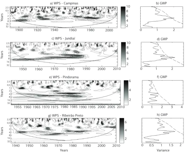
Based only on the frequency domain, the spectral analysis of the SPI signals, carried out for the series of Campinas, Pindorama and, Ribeirão Preto, has indicated a concentration of power in the (≈) 4 year band (note that only the global wavelet power of Campinas - Figure 3b - shows a variance peak above the 5% significance level). In addition, it is also worth emphasizing the presence of a significant peak of wavelet energy in the 4-6 year band in the SPI signal of Jundiaí. However, extending this ap-proach to the time-frequency domain, it can be observed (Figure 3a,c,e,g) a decrease in the wavelet energy after the beginning of the 1990’s. It is also worth emphasizing that in the location of Campinas, there is another period in which a low level of wavelet energy can also be verified (1935-1960; Figure 3a). Thus, considering that after the beginning of the 1990’s no variance peak was observed in the 3-6 year band, and also considering that in the lon-gest data record of this study no significant wavelet power (≈ 4 band) was observed during (approximately) 25 years (1935-1960), the establishment of a dominant mode for the SPI temporal variability becomes (at least) unrelia-ble. Finally, it is interesting to realize that although only
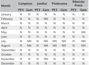
Table 1. Evaluating the normality assumption of the Standardized Precipitation Index series (State of São Paulo, Brazil). N is associated with standard normal distribution. NN is associated with nonnormal distributions. The index calculations were based on Pearson type III distribution (PE3) and on gamma 2-parameters distribution (Gam)
Month Campinas Jundiaí Pindorama
Ribeirão Preto PE3 Gam PE3 Gam PE3 Gam PE3 Gam
January N N N N N N N N
February N N N NN N N N N
March N N N N N N N N
April N N N N N N N N
May N N N N N N N NN
June N N N N N N N N
July N NN N NN NN NN N NN
August N NN N NN NN NN N NN
September N N N N N N N N
October N N N N N N N N
November N N N NN N N N N
December N N N N N N N N
Table 2. Mean (M), standard deviation (SD) and frequency of occurrence of zeros of four monthly rainfall series of the State of São Paulo, Brazil
Month Campinas Jundiaí Pindorama Ribeirão Preto
M SD Freq0 M SD Freq0 M SD Freq0 M SD Freq0
January 249 100.1 0.0 243 91.8 0.0 258 101.2 0.0 279 106.0 0.0
February 200 87.4 0.0 188 77.4 0.0 213 105.3 0.0 219 101.0 0.0
March 153 70.1 0.0 159 70.5 0.0 156 75.0 0.0 166 76.3 0.0
April 64 44.5 0.0 66 40.3 2.9 70 52.3 3.3 73 56.5 135.1
May 58 47.6 2.5 65 54.4 2.9 60 51.2 5.0 55 46.8 405.4
June 47 43.5 6.6 52 52.8 2.9 31 35.2 16.7 27 31.9 1891.9
July 31 37.6 12.4 44 45.5 13.0 24 30.2 26.7 22 28.2 2162.2
August 33 33.4 14.0 34 37.3 14.5 27 34.0 20.0 20 31.1 3108.1
September 67 52.5 0.8 69 59.6 1.4 59 50.4 6.7 53 51.4 405.4
October 119 62.5 0.0 126 56.9 0.0 113 55.9 0.0 123 60.5 0.0
November 149 67.9 0.0 146 68.1 0.0 133 65.6 0.0 172 72.0 0.0
1940 1950 1960 1960 1955 1965 1970 1970 1975 Years Variance
g) WPS - Ribeirão Preto e) WPS - Pindorama
c) WPS - Jundiaí
a) WPS - Campinas b) GWP
d) GWP f) GWP h) GWP 1980 1980 1985 1980 1990 1990 1995 1990 2000 2000 2005 2000 2010 2010 2010
0 1 2
0 1 2
0
0 0.5 1.5
1
1 2
2
3 4
1950 1960 1970
1940 1920
1900 1960 1980 2000
2 4 2 4 6 6 8 10 8 10 2 4 6 6 2 4 0,5 2,5 1 2 4 8 16 32 0,5 2,5 1 2 4 8 16 32 0,5 2,5 1 2 4 8 16 32 0,5 2,5 1 2 4 8 16 32 Y ears Y ears Y ears Y ears
Figure 3. Wavelet power spectrum (WPS) of four Standardized Precipitation Index series of the State of São Paulo, Brazil. Global Wavelet Power Spectrum (GWP - in variance units).
monthly SPI series are being addressed in this study, it is worth emphasizing that increasing the wavelet scale can be seen as a similar procedure of increasing the SPI time scale calculation. Both signals will respond more slowly to changes in rainfall amounts as the scale of their calcula-tions becomes larger.
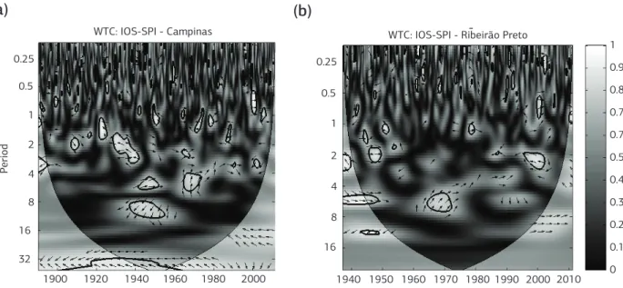
As previously discussed, according to Grinsted et al. (2004) the squared wavelet coherence of two processes that may be linked to each other by some geophysical reason tends to exhibit a constant phase relationship wi-thin several time scales. In this view, the results depicted in figure 4 (Campinas and Ribeirão Preto) indicate no remarkable relationship between the temporal variabi-lity of the SPI and the ENSO signal. It can be verified that regions of figure 4 with significant coherence occur during short periods of time. In addition, even within these regions no consistent phase relationship can be observed between these both physical signals. The same features were observed (not illustrated) in the locations of Jundiaí and Pindorama. Thus, at least under a sta-tistical point of view, the use of the ENSO signal in
predicting possible drought conditions in these four lo-cations can result in unreliable information. This last statement seems to agree with previous studies that also indicate the lack of a statistically significant ENSO in-fluence over the rainfall variability of the State of São Paulo (Rao and Hada, 1984; Blain et al., 2009; Blain and Kayano, 2011).
a p-value ≤ 0.10, has occurred on the months of June in Pindorama. Considering the last 60 years (Table 4), only four cases associated with p-values ≤ 0.10 are observed: Jundiaí (January and November), Pindorama (January) and, Ribeirão Preto (October).
However, before indicating the absence of any evi-dence of climate trends in the SPI series, it is important to recall that according to Yue and Hashino (2003), al-though the critical level usually adopted for rejecting the H0 associated with the MK is p-value=0.05, for (really) trend-free samples the final value of this test should be near to zero. The corresponding p-value should be close to 0.5. In addition, Radziejewski and Kundzewicz (2004) states that even when no significant trend has been detec-ted by statistical tests, this cannot ensure the absence of
Figure 4. Squared wavelet coherence between the Southern Oscillation Index (SOI) and the Standardized Precipitation Index (SPI) obtained from the weather stations of (a) Campinas and (b) Ribeirão Preto (State of São Paulo, Brazil). The regions in which the 5% significance level was achieved are represented by the thick lines. An arrow pointing vertically upward is obtained when the SPI series lags the SOI series by 90º. An arrow pointing from left to right (horizontal) is obtained when the series are in-phase.
0.25
WTC: IOS-SPI - Campinas
1900 1920 1940 1960 1980 2000 1
2
4
8 0.5
16
32
P
eriod
(a)
0.9 0.25
WTC: IOS-SPI - Ribeirão Preto
1940 1950 1960 1970 1980 1990 2000 2010 1
1
2
4
8
0.8
0.7
0.7
0.5 0.5
16
0.4
0.3
0.2
0.1
0
(b)
any form of change in the time series. According to these authors, statistical evaluations may fail in detecting weak changes and/or changes which have occurred in the final years of the time series under analysis.
Considering these last two statements, it becomes im-portant to verify that according to the Pettitt test (Table 4) the beginning of a (decreasing) trend in the SPI series of Campinas and Ribeirão Preto (months of October; p--value < 0.10) was detected as being the years of 1983/84. The same feature is observed in the series of Jundiaí and Pindorama (months of October), although with p-values greater than 0.20. The MK final values obtained from the-se four weather stations for the monthly the-series of October were always negative. Furthermore, it is worth emphasi-zing that a climate change that can severely impact the
Table 3. Mann-Kendall test applied for series of the Standardized Precipitation Index. State of São Paulo, Brazil
Month Campinas Jundiaí Pindorama RibeirãoPreto
1890-2010 1942-2010 1951-2012 1937-2013
MK p-value MK p-value MK p-value MK p-value
January 0.52 0.61 1.84 0.07 1.95 0.05 0.40 0.69
February -0.94 0.35 -0.95 0.34 -0.55 0.58 0.27 0.79
March -0.16 0.87 -0.01 0.99 0.14 0.89 -0.62 0.54
April 0.74 0.46 0.81 0.42 1.49 0.14 0.38 0.71
May 1.04 0.30 2.86 <0.01 1.05 0.30 2.22 0.03
June -0.56 0.58 -0.61 0.54 -1.74 0.08 -0.19 0.85
July 1.05 0.29 1.47 0.14 1.17 0.24 1.08 0.28
August -1.53 0.13 0.80 0.42 -0.39 0.70 0.54 0.59
September -0.62 0.54 2.07 0.04 1.23 0.22 1.95 0.05
October -0.33 0.74 -0.06 >0.90 -0.73 0.47 -1.52 0.13
November -0.89 0.37 1.38 0.17 0.80 0.42 0.57 0.57
agricultural activities of the State of São Paulo, has already been described by Dufek and Ambrizzi (2007). Based on the evaluation of indices derived from 59 daily pre-cipitation series, these authors described an increasing trend in the number of consecutive dry days observed in the aforementioned State. Also according to Dufek and Ambrizzi (2007) this climate change has occurred after 1985 (very close to the change point -1983/84- observed in this study).
Thus, it can be pointed out that the variability obser-ved in the SPI series during the transition period between the dry and the rainy seasons of the State of São Paulo cannot be seen as the result of a purely random process. In other words, it is unlikely that this concentration of nega-tive MK values (Tables 2, 3 and 4; months of October), is just a product of chance.
4. CONCLUSION
The Pearson type III distribution was better than the gamma 2-parameter distribution, in providing monthly SPI series closer to the normality assumption inherent to the use of this probabilistic standardized index.
The spectral analyses used in this study did not allow us to establish a dominant mode in the SPI time series.
Moreover, no remarkable relationship between the tem-poral variability of this drought index and the ENSO sig-nal was observed.
In general, the trend tests indicated the presence of no significant trend components in the SPI series. However, the results obtained from these trend tests have also indi-cated that the temporal variability of the SPI, observed at the months of October over the last 60 years, cannot be seen as the result of a purely random process. This last inference is due to the concentration of decreasing trends, with a common beginning (1983/84), in the four SPI se-ries of the study. Thus, the hypothesis of the presence of climate changes in these series cannot be rejected.
REFERENCES
ABRAMOWITZ, M.; STEGUN., I.A. Handbook of mathematical function. New. York: Dover Publications, 1965. 1046p.
BLAIN, G.C.; PIEDADE, S.M.S.; CAMARGO, M.B.P.; GIAROLLA, A. Distribuição temporal da precipitação pluvial mensal observada no Posto Meteorológico do Instituto Agronômico, em Campinas, SP. Bragantia, v.66, p.347-355, 2007.
BLAIN, G.C. Considerações estatísticas relativas à oito séries de precipitação pluvial da Secretaria de Agricultura e Abastecimento
Table 4. Mann-Kendall test and Pettitt test applied for four Standardized Precipitation Index series of the State of São Paulo (common period of 1951-2010)
Month Campinas Jundiaí Pindorama Ribeirão Preto
MK p-value MK p-value MK p-value MK p-value
January 0.83 0.41 1.66 0.10 1.95 0.05 0.81 0.42
February -0.47 0.64 -0.04 0.96 -0.55 0.58 0.00 1.00
March 0.21 0.83 0.87 0.39 0.14 0.89 -0.84 0.40
April -0.15 0.88 -0.14 0.89 1.49 0.14 -0.13 0.90
May 1.44 0.15 1.54 0.12 1.05 0.30 0.98 0.33
June -0.54 0.59 -0.71 0.48 -1.74 0.08 -1.57 0.12
July 1.07 0.29 1.60 0.11 1.17 0.24 0.74 0.46
August -1.02 0.31 -0.66 0.51 -0.39 0.70 -0.68 0.49
September 0.84 0.40 1.45 0.15 1.23 0.22 1.49 0.14
October -1.40 0.16 -1.14 0.26 -0.73 0.47 -2.21 0.03
November 0.59 0.55 2.20 0.03 0.80 0.42 0.87 0.39
December 0.79 0.43 0.53 0.60 0.33 0.74 -0.29 0.77
Month Pettitt p-value Pettitt p-value Pettitt p-value Pettitt p-value
January 1987 >0.9 1987 0.17 1982 0.09 1999 >0.9
February 1977 0.76 1982 >0.9 1966 0.95 2005 >0.9
March 1982 0.50 1985 0.33 1993 0.59 1963 >0.9
April 1997 >0.9 1996 0.44 1972 0.33 1994 >0.9
May 1983 0.11 1976 0.08 1976 0.21 1983 0.21
June 1984 0.65 1984 0.85 1984 0.29 1984 0.28
July 1964 0.80 1970 0.55 1964 0.55 1964 0.77
August 1987 0.47 1987 >0.9 1991 >0.9 1991 >0.9
September 1970 0.51 1976 0.29 1965 0.33 1975 0.21
October 1983 0.08 1984 0.23 1984 0.32 1984 0.02
November 1972 >0.9 1972 0.07 1975 0.21 1966 >0.9
do Estado de São Paulo. Revista Brasileira de Meteorologia, v.24, p.12-23, 2009.
BLAIN, G.C.; KAYANO, M.T.; CAMARGO, M.B.P.; LULU, J. Variabilidade amostral das séries mensais de precipitação pluvial em duas regiões do Brasil: Pelotas-RS e Campinas-SP. Revista Brasileira de Meteorologia, v.24, p.1-11, 2009.
BLAIN, G.C. Detecção de tendências monótonas em séries mensais de precipitação pluvial do Estado de São Paulo. Bragantia, v.69, p.1027-1033, 2010.
BLAIN, G.C.; KAYANO, M.T. 118 anos de dados mensais do Índice Padronizado de Precipitação: série meteorológica de Campinas, Estado de São Paulo. Revista Brasileira de Meteorologia, v.26, p.137-149, 2011.
DUFEK, A.S.; AMBRIZZI, T. Precipitation variability in Sao Paulo State, Brazil. Theoretical and Applied Climatology, v.93, p.167-178, 2007.
EDWARDS, D.C.; McKEE, T.B. Characteristics of 20thcentury drought in the United States at multiple time scales. Fort Collins: Colorado State University, 1997. 155p. (Atmospheric Science Paper, nº 634, Climatology Report nº 97-2)
FERNANDES, D.S.; HEINEMANN, A.B.; PAZ, R.L.F.; AMORIM, A.O. Desempenho de índices quantitativos de seca na estimativa da produtividade de arroz de terras altas. Pesquisa Agropecuária Brasileira, v.45, p.771-779, 2010.
GRINSTED, A.; MOORE, J.C.; JEVREJEVA, S. Application of the cross wavelet transform and wavelet coherence to geophysical time series. Nonlinear Processes in Geophysics, v.11, p.561-566, 2004.
GUTTMAN, N.B. On the sensitivity of sample L moments to sample size. Journal of Climatology, v.34, p.113-121, 1994.
GUTTMAN, N.B. Accepting the “Standardized Precipitation Index”: a calculation algorithm Index. Journal of the American Water Resources, v.35, p.311-322, 1999.
KAYANO, M.T.; SANSÍGOLO, C. Interannual to decadal variations of precipitation and daily maximum and daily minimum temperatures in southern Brazil. Theoretical and Applied Climatology, v.97, p.81-90, 2009.
KENDALL, M.G.; STUART, A. The advanced theory of statistics. 2.ed. Londres: Charles Griffin, 1967. v.2, 690p.
KUNDZEWICZ, Z.W.; ROBSON, A.J.; Change detection in hydrological records— a review of the methodology. Hydrological Sciences Journal, v.49, p.7-19, 2004
LI, W.; FU, R.; JUAREZ, R.I.N.; FERNANDES, K. Observed change of the standardized precipitation index, its potential cause and implications to future climate change in the Amazon region. Philosophical Transactions of the Royal Society, v.363, p.1767– 1772, 2008.
LIVIDA, I.; ASSEMAKOPOULOS, V.D.; Spatial and temporal analysis of drought in Greece using the Standardized Precipitation Index (SPI). Theoretical and Applied Climatology, v.89, p.143-153, 2007.
MACEDO, M.J.H.; GUEDES, R.V.S.; SOUZA, F.A.S.; DANTAS, F.R.C. Análise do índice padronizado de precipitação para o Estado da Paraíba, Brasil. Revista Ambiente & Água, v.5, p.204-214, 2010.
MCKEE, T.B.; DOESKEN, N.J.; KLEIST, J. The relationship of drought frequency and duration to the time scales. In: CONFERENCE ON APPLIED CLIMATOLOGY, 8., 1993, Anaheim. Proceedings… Boston: American Meteorological Society, 1993. p.179-184.
MANATSA, D.; MUKWADA, G.; SIZIBA, E.; CHINYANGANYA, T. Analysis of multidimensional aspects of agricultural droughts in Zimbabwe using the Standardized Precipitation Index (SPI). Theoretical and Applied Climatology, v.102, p.287-305, 2010.
MISHRA, A.K.; SINGH, V.P.; DESAI, V.R.; Drought characterization: a probabilistic approach. Stochastic Environmental Research Risk Assessment, v.23, p.41-55, 2007.
PALMER, W.C. Meteorological drought. Washington: U.S. Department of Commerce, 1965. 58p. (U.S. Department of Commerce. Research paper, 45)
PETTITT, A.N. A non-parametric approach to the change-point problem. Journal of the Royal Statistical Society, v.28, p.126-135, 1979.
PEZZI, L.P.; KAYANO, M.T. An analysis of the seasonal precipitation forecasts in South America using wavelets. International Journal of Climatology, v.29, p.1560-1573, 2009.
RADZIEJEWSKI, M.; KUNDZEWICZ, Z.W. Detectability of changes in hydrological records. Hydrological Sciences Journal, v.49, p.39-51, 2004.
RAO, V.B.; HADA, K. An experiment with linear regression in forecasting of spring rainfall over south Brasil. Atmosfera, v.7, p. 83 -87, 1994.
REBOITA, M.S.; KRUSCHE, N.; PICCOLI, H.C. Climate variability in Rio Grande, RS, Brazil: A quantitative analysis of contributions due to atmospheric systems. Revista Brasileira de Meteorologia, v.21, p. 256-270, 2006.
SANSIGOLO, C.A. Análise comparativa do desempenho dos Índices de Seca de Palmer (PDSI) e da Precipitação Normalizada (SPI) em Piracicaba, SP (1917 – 2001). Revista Brasileira de Meteorologia, v.19, p.51-56, 2004.
STEINSKOG, D.J.; TJØSTHEIM, D.B.; KVAMSTØ, N.G. A cautionary note on the use of the Kolmogorov–Smirnov test for normality. Monthly Weather Review v.135, p.1151-1157, 2007.
TADESSE, T.; WILHITE, D.A.; MICHAEL J. HAYES, M.J. Discovering Associations between Climatic and Oceanic Parameters to Monitor Drought in Nebraska Using Data-Mining Techniques. Journal of Climate, v.18, p.1541-1550, 2005.
VLČEK, O.; HUTH R. Is daily precipitation Gamma-distributed? Adverse effects of an incorrect application of the Kolmogorov-Smirnov test. Atmospheric Research, v.93, p.759-766, 2009.
WILKS, D.S. Statistical methods in the atmospheric sciences. 2.ed. San Diego: Academic Press, 2006. 629p.
WU, H.; HAYES, M.J.; WILHITE, D.A.; SVOBODA, M.D. The effect of the length of record on the Standardized Precipitation Index calculation. International Journal of Climatology, v.25, p.505-520, 2005.
WU, H.; SVOBODA, M.D.; HAYES, M.J.; WILHITE, D.A.; WEN, F. Appropriate application of the Standardized Precipitation Index in arid locations and dry seasons. International Journal of Climatology, v.27, p.65-79, 2007.
YUE, S.; HASHINO, M. Temperature trends in Japan: 1900-1996. Theoretical and Applied Climatology, v.75, p.15-27, 2003.
YUE, S.; HASHINO, M. Probability distribution of annual, seasonal and monthly precipitation in Japan. Hydrological Sciences Journal, v.52, p.863-877, 2007.
ZHAI, J.; SU, B.; KRYSANOVA, V.; TOBIAS, VETTER, T.; GAO, C.; JIANG, T. Spatial variation and trends in PDSI and SPI indices and their relation to streamflow in ten large regions of China. Journal of Climate, v.23, p.649-663, 2010.