1
I~DAÇÃO
GETUUO VARGAS
, "Praia de Botafogo, nO 190/10" andar - Rio de Janeiro - 22253-900
Seminários de Pesquisa Econômica 11
(la
parte)
11
CENTRAL BANK
AUTO NO MY , THE EXCHANGE
RATE CONSTRAINT AND
\marf.
MARCIO RONCI
(International Monetary Fund)
Coordenação: Prof. Pedro Cavalcanti Ferreira Tel: 536-9353
I.
_
; J.; ! \ ... : ~ c: ~L! V ·,F:G,.\S _.~,. "-~~~F3A1J/Jf
ÇJ]fII
~i-..
Central Bank Autonomy, the Exchange Rate Constraint and Inflation:
the case of Italy, 1970 - 1992
by Giuseppe Tullio and Mareio Ronei1 2
Introduction
ltalian inflation was relatively high and variable in the 1970's and early 1980's peaking three times at around 20% per year, mainlyas a result of excessive monetary financing of increasing budget deficits, two oil shocks (1974,1980) and one major exchange rate shock (1976). The substitution of a more independently minded Central Bank governor in 1975 (Paolo Baffi) led slowly to significant changes frrst in the financiaI system (development of the Treasury bill and bond market, started in 1976), then in the behaviour of the Central Bank towards the monetary financing of the governrnent in 19773 and finally to an important institutional change which increased the independence of the ltalian Central Bank, the so-ca1led divorce of July 1981 between the Bank and the Governrnent. The latter freed the Bank from the compulsory purchase of unsold Treasury bills and bonds in the primary market. Another important institutional change was the creation of the European Monetary System (EMS) in March 1979, which by linking the lira to the Deutsche Mark made it a lot easier for the ltalian Central Bank to convince the Governrnent to change interest rates when the currency was under attack.
The increased autonomy ofthe Banca d'ltalia in the course ofthe 1980's and the move towards flXed exchange rates within the Exchange Rate Mechanism (ERM) of the EMS are two processes which went hand in hand and it is difficult to tell precisely which caused which. Put differently, were the development of the ltalian secondary market for Treasury bonds and the July 1981 divorce at the root of the increased credibility of the lira -DM exchange rate in the course of the 1980's or was it the ERM constraint which led the Banca d'ltalia to demand greater autonomy and the Minister of Finance to grant it? The answer is probably both. Be that as it may, it is beyond any doubt that both greater autonomy and the exchange rate constraint were crucial factors in the fight against inflation.
Two additional important institutional changes carne into effect in the early 90s after the signature of the Maastricht Treaty (1991) : decisions about changes in the discount rate became in 1992 the sole responsibility of the Bank of ltaly, while before they were decided by the Minister of Finance and the so-ca1led "Conto corrente di Tesoreria", a very large overdraft facility of the
lGiuseppe Tullio is professor of Economics at the U niversity of Brescia and member of the Scientific Committee of the Osservatorio e Centro Studi Monetari of Luiss University, Rome. Mareio Ronei is an economist of the International Monetary Fund. The opinions expressed in this pape r are those of the authors and do not necessarily reflect those of the IMF. This paper is based on a much longer paper on ltalian and Brazilian inflation written by the same authors and circu1ated as an EPGE working paper of the Fundacao Getulio Vargas in Rio and as a LUISS University working paper
in Rome (fullio and Ronci,1994).
lne authors benefitted from discussions with Joachim Levy, Fernando de Holanda Barbosa, Renato Fragelli, Pasquale Scandizzo, Franco Spinelli and ananonymous referee ofthisjournal. Giuseppe Tullio gratefully acknowledges the financial support of the ltalian National Seience Foundation (CNR) and the Brazilian counterpart (CNPq). The paper was written while the first author was visiting fellow at the Fundação Getulio Vargas in Rio de Janeiro.
3For a deeper analysis of the views of Governor Baffi on inflation and on bis crucial role in starting the changes wbich finally led to the control of ltalian inflation see Spinelli and Fratianni (1991).
Treasury at the Central 8ank of up to 7 - 8 per cent of GDP on which the Treasury was paying only 1 % interest. was abolished on January 1st 19944. In the case of these additional institutional innovations it is cJear that the main stimulus carne from the signature of the Maastricht Treaty at the end of 1991.
These changes, coupled with the increased consciousness of the public and policy makers that inflation is a negative phenomenon, made it possible for ltaly to control inflation in the course of the 1980's and by November 1994 inflation was around 3.8 percent per year, about one percentage point more than in West Germany, despite the fact that ltalian nominal budget deficits have exceeded 10% of GDP for the whole 1980's and were still around the same order of magnitude in 1994.
This paper analyzes the determinants of inflation in Italy over the period 1970-1992 with particular emphasis on the role of central bank autonomy in influencing monetary growth and on the role of monetary growth and of the EMS in influencing inflation. We shall see how radically the determinants of inflation changed in the course of the period: in the 1970s and early 80s, when central bank dependence from the governrnent was high and lor the ERM of the EMS was still not very credible, monetary growth was highly unstable and it was the main determinant of inflation. Tests of an amended version of the quantity theory of money which allows for oil price shocks turn out to be very satisfactory. After the March 1983 general realignrnent and the French V- turn, the ERM became more credible and monetary growth stopped being a significant determinant of inflation. After March 1983 German inflation, current and lagged, became instead the main variable influencing Italian inflation. The timing of this radical change in the determinants of Italian inflation was unveiled by means of Cusum of squares tests, break-point Chow tests and recursive parameter estimates.
The paper is divided as folIows. Section 1 is devoted to a brief analysis of the main institutional changes affecting the Banca d'Italia's autonomy from 1970 to 1994. Section 2 presents a very simple model of inflation in which monetary policy is its the main driving force (the quantity theory) , but supply shocks (oil and taxes) and inertial factors are also important. In turn money growth is caused by budget deficits, balance of payments surpluses, the business cycle and/or inflation. The estimates of the reaction function of Italian monetary authorities are presented in Section 3. Section 4 presents the estimates of the inflation equation for the whole sample period on which then a series of stability tests are performed (Cusum of square test, break-point Chow test and recursive parameter estimates). They alI suggest a structural break in the inflation equation in the second quarter of 1983, just after the general realignrnent of March 1983 and the French V-turn
which are believed to have made the exchange rate mechanism (ERM) of the EMS more credible .. The quantity theory is then reestimated for the period from the the beginning of floating around 1973 to the frrst quarter of 1983. For the period from the 2nd quarter of 1983 to the beginning of 1992 the determinants of Italian inflation changed completely as German inflation became more and more important and the Italian money stock lost alI its explanatory power. This German dominance hypothesis of Italian inflation (Model 2) is tested for the second period. By performing non-nested encompassing F-tests we also show that for this second period Model 2 is clearly superior to the quantity theory (Model 1). Section 5 concludes.
The inflation equation and reaction function estimated support the amended quantity theory
4with the same law, also decisions about changes in reserve requirements became to a large extent the responsibility of the Bank.
..
explanation of inflation for ltaly from 1973 to 1983 (Model 1). In addition they support what Spinelli calls the "fiscal dominance hypothesis" of inflation (Spinelli and Fratianni, 1991 and Favero and Spinelli, 1992) only up to the end of 1977. As to the post March 1983 period we show that the German dominance hypothesis (Model 2) clearly outperformed the quamity theory (Model 1).
1. Changes in the Italian monetary constitution since 1945: a brief overview
Even through institutional changes do not always influence immediately monetary growth and inflation, increased autonomy represents an environrnent more conducive to lower inflation, as has been the case for ltaly in the course of the two decades under analysis. However, Central Bank autonomy is neither a sufficient nor a necessary condition for low inflation. lt is not a necessary condition because a Central Bank totally lacking independence can guarantee low inflation in the absence of major fiscal, oil or Iabour market shocks, as has been the case in Italy in the 1950s and early 1960s. It is not a sufficient condition because a fully independent Central Bank can make mistakes or decide independently from governrnent pressure to engenier a quick economic recovery by inflating.
The Italian Central Bank (Banca d'Italia) has been de facto rather dependem from the Governrnent up until the so-called "divorce" of July 1981 which relieved the Bank from compuIsory purchase of unsold treasury bills and governrnent bonds in the primary marke~. The negative consequences of this compuIsion for the controI of the monetary base were enhanced by the Iack of a developed secondary governrnent security market until 1976.
The development of this market which started in 1976, the joining of the ERM in March 1979, albeit with a Iarger margin (+ 6 percent) than other members (+ 2.25 percent), 6 the divorce in July 1981, the abolition of capital controIs, achieved by march 1990, represent important changes in the direction of more independence from the Governrnent and grater acceptance of German anti-inflationary policies. Passacantando (1994) argues that also the development of the screen-based secondary market for Governrnent bonds and the reform of the auction system of governrnent bonds and bills, both of which occured only sIowly in the course of the second half of the 1980's, played an important role in enhancing the controllability of monetary aggregates.
More recently, in connection with the obligations of the Maastricht Treaty signed in 1991 other measures were taken. In 1992, discount rate changes became the sole responsibility of the Bank of Italy, while before they were decided by the Finance Minister after consultation with the Governor of the Bank of Italy. The reform of the "conto corrente di Tesoreria" (the overdraft facility of the Treasury on its account with the Bank of Italy) carne into effect on January 1st 1994, together with greater autonomy on the part of the Bank in determining reserve requirements .
5Visco agrees that with the 1981 divorce the Bank became • de facto· independent and argues that it reached legal independence only with the 1992/94 reforms. The July 1981 divorce was only an agreement between the bank and the Treasury; it was not a law approved by Parliament.
6rbe margin was reduced to + 2.25 percent on January 1st 1991 and remained at this levei until the lira left the ERM on Seotember. 16th. 1992.
From the late 1940's to 1993 the overdraft facility could not exceed 14 percent of planned budgetary expenditures for the year. With the large annual nominal increases in governrnent expenditures, especially in the 1970's and 1980's, this facility represented a major channel through which monetary base was created. lt is worth pointing out that the interest cost to the Treasury on the overdraft is only 1 percent, and it goes without saying that the Treasury has generally tendend to make use of it up to the legal ceiling. In the last year of its existence the facility amounted to over 7 per cent of GOP.
According to the law of January 4th 1945, later amended on April 19th 1948 the Governor and the other three members of the Directorium (the Director General and two Oeputy Oirectors General) are proposed by the Board of the Bank (Consiglio Superiore) to the Council of Ministers. After approval by the Council ofMinisters, the President ofthe Republic nominates the Governor (members of the Directorium). Thus alI higher positions of the Bank are political nominations. However, there is no time limit to the appointments nor a compulsory age of retirement. However, there is a debate going on about the introduction of limits.
The "de facto" dependence of the Bank of ltaly from the Government changed substantially from 1945 to 1981, despite a roughly unchanged legal framework; the economic philosophy of the Governor, the size of the budget deficits to be financed, as well his personality and politicaI sympathies played a big role. As pointed out by Spinelli and Fratianni (1991), the ltalian post-war period can be divided into three sub-periods: the frrst one from the stabilization of 1947 to 1960 under Governor Menichella, the second one under Governor Carli (1960 to 1975), the third one under Baffi (1975-80) and Ciampi (1980-1993). Fazio, appointed in 1993, is the Iast governor. As can be seen, ltaly had only five governors since 1947, a very smalI turnover.
During the frrst period price stability was an important objective of the Bank, monetary policy was geared towards the medium to Iong run and the controI of the supply of money was also considered important. Money was assumed to influence prices and the balance of payments, in line with the classical view.
During Carli's period the increase in employment was considered more important than the controI of inflation, inflation was partly viewed as fostering economic growth, money was not considered to play a role in controlling inflation, the Iatter being considered to be mostly of a cost-push type. As a result monetary policy became incapable to counteract the destabilizing shocks that hit the ltalian economy during this period (wage, fiscal and oil shocks); worse than that, according to Spinelli and Fratianni, it becomes itself a source of instability. From a market oriented monetary policy during Menichella's period, ltaly moved to direct credit and exchange controIs, an almost total financiaI isolation of the country from abroad 7 and at times a stubborn controI of nominal interest rates which were kept much too Iow to controI inflation (Fig. 1), mainly to please the political forces backing the governrnents and thriving on Iarge and increasing budget deficits. The real interest rate dropped to about minus 9 percent in 1974 and again to about minus 5 percent in 1976 and 1980.
It should not be forgotten that of the five governors mentioned above only Carli joined the Bank as Director General barely a year before the appointment as Governor of the Bank. The others started their career in the Bank at a relatively early age.
•
. The third period, which started in 1975 with Baffi, represents a reversal towards the dassical school, although it took a very long time to dismantle controls on credit and foreign exchange transactions, to regain enough flexibility in leading interest rates, to implement control of monetary aggregates and to reduce inflation to acceptable leveis. Baffi also had to face budget deficits that were among the highest in Italian post-war history (about 13 percent of GDP in 1978, see Fig. 2). However, only Ciampi managed to complete .the work started by Baffi, despite the increasing constraints coming from public finances. 8 The change in the Bank's objectives can be best summarized by Ciampi' s statement in May 1981:
"The retum to a stable currency requires a real
change in the monetary constitution( ... ) The ftrst condition is that the power to create money should
be completely independent from the agents that determine expenditure". 9
After the divorce of July 1981 Italian real interest rates became positive and high, hovering around 5 percent per year for the rest of the eighities and early nineties. In addition, compared to the seventies, they were very stable (Fig. 1). The exchange rate constraint of the ERM and a gradual capital flow liberalization, completed in 1991, certainly helped in this respect. The high real interest rates managed to break the vicious circle running from high budget deficits to high money growth. The latter declined sharply in the 1980's despite continuing high budget deficits and it stopped to a large extent leading inflation and its turning points as it had done in the 1970's.
It is too early to telI whether the beginning of Fazio's mandate will represent a change in the economic philosophy of the bank. It is certain, however, that with fulI autonomy and perfect flexibility of exchange rates the powers of the Bank as welI as its responsibilities concerning inflation have increased substantially.
Table 1 - Today's ltalian Monetary Constitution: maio features
1) The Central Bank does not have 5) Tha Bank is not compelled to finance
statutory responsability to stabilize prices. government deficits since the "Divorce" in 1981.
2) The Governor cannot be dismissed and 6) The overdraft facility of the Treasury at
has a lifetime mandate. the Banca d'Italia was abolished in 1994.
3) the Governor is proposed by the Board 7) The Central Bank has the sole
of the Bank, approved by the Council of responsibility of discount rate changes
Ministers and nominated by the President since 1992 and of reserve requirement
of the Republic. changes since 1994.
4) Staff is well prepared. The Bank has one of the best research departments in
Europe. The Bank provides the
governrnent with economic advice .
8In 1992 the govemment budget deficit and total public debt out standing were still about 10 and 110 percent of GDP, !,CSpeCtively.
The historical evidence presented suggests that the degree of independence of the monetary authority is an important factor to explain the different inflation performance of ltaly in the 1970's and 1980's; while in the 1970's and early 1980's ltalian inflation peaked three times at over 20%, in the course of the 1980's it was slowly brought under control and by November 1994 it had fallen to 3.8%. However, it took a very long time for the changes in the monetary constitution and for the ERM to fully excert their impact on monetary growth and inflation. In other words it seems that in the case of ltaly important changes in the monetary constitution did not have an immediate impact on the behaviour of the Central Bank and on the determinants of inflation. We sha1\ see below that the degree of monetary financing of the government budget deficit changed 3-4 years before the divorce of 1981 and that the actual determinants of inflation changed about two years later.
2. A Model of inflation and the Central Bank's reaction function
We assume that inflation is determined by costs of production as well as aggregate demand, in particular monetary policy. For Italy it has been shown that wage dynamics, indexation rules and oH shocks play an importaot role. In addition monetary policy and velocity changes are considered crucial. lO In Italy the tax pressure increased substantially especially in the 1980's; therefore also direct and indirect tax changes were included among the explanatory variables.
Equation (1), says that inflation is determined by the rate of growth of nominal wages corrected for productivity growth and by the rate of change of the price of oH expressed in domestic currency
where: D = frrst difference operator
p = log of the price leveI measured by the consumer price index q = log of productivity of labour
w = log of nominal wage
p* oH = log of the price of oH in US dollars
s = log of the exchange rate of the domestic currency with the US$ u = other cost shocks like agricultural price, tax' cost of capital
shocks and foreign inflation
The Phillips curve is given by: n
(2) DWt
=
Dqt+
k ai DPt-i+
{3 ht i= 1where: ht = output gap, measured as % deviation from potential output
The demand side of the economy is assumed to be influenced by the rate of growth of money, adjusted for changes in real GDP and in the real money demand ("quantity theory"). Substituting (2) into (1) and taking into account the demand factors mentioned above one obtains the final equation for inflation:
(3)
where:
n
DPt = bo
+
b 1 Dmt - b2 DYt+
E b3 i DPt-i+
b4 ht+
b5 Dpoilt+
i= 1 '
m = log of the stock of money
e = demand shock
y = log of real GDP
and where a constant term bo has been added andpoil is expressed in domestic currency (P*oil+s).
All coefficients are expected to be positive and most explanatory variables are expected to influence inflation with lags which we introduced explicitly in (1) - (3) only for inflation to simplify the notation. The significance of the coefficients of lagged inflation in equation (3) will provide an indirect test of the so-called "inertia hypothesis" of inflation and
b 1
= 1 will provide a test for the "quantity theory " hypothesis.Money is not assumed to be exogenous. The central bank is assumed to react with lags to the governrnent budget deficit, past inflation, the development of externaI accounts (either the balance of payments or the current account) and the business cycle. Thus the reaction function of the central bank is given by:
where: g = nominal governrnent budget deficit divided by GDP
bopy = balance of payments or current account divided by GDP
The idea behind introducing the externaI accounts into the reaction function (4) is that when they are in surplus the central bank feels more relaxed about reducing interest rates and expanding money or more simply that it behaves passively by the "rules of the game" and does not sterilize
completely international reserve flows: c3 is therefore assumed to be positive. So is cf' As·to the reaction to inflation and the business cycle the central bank can either behave in an accomodating way
(c2' c4
>
O) or in a stabilizing way (c2' c4< O). In the next section we present estimates of the reaction function (4) and in Section 4 we present estimates of the inflation equation (3).3. The reaction function of Italian monetary authorities
The main hypothesis we want to test in this Section is that monetary policy (and hence inflation) are dominated by fiscal policy (fiscal dominance model). In order to test this hypothesis we estimated a general version of the monetary authority reaction function (equation (4) of section 3) with 4 lags for each variable and then simplified it using F-tests, according to Hendry's method.
For Italy we have reliable quarterly data from the beginning of the 1970's; hence our estimates cover the period 1971.2 to 1992.1 (the last observation available). Five observations are lost at the beginning owing to the way we have defined percentage changes (with respect to the same quarter of the previous year) and to lags. D 4m2 is defined as log m2 -log m2t-4' It is therefore a rate of change with respect to the same quarter of the previous year. AlI percentage changes are defined in this way. Changes of nominal variables with respect to the previous quarter tend to be dominated by seasonal factors and contain therefore too much noise. Seasonality has also changed substantially in ltaly in the course of the sample period.
The estimated reaction function for ltaly is:
Regr. (1) D4m2t = 0.01 + 0.80 D4m2t_l + 0.11 Gt + 0.22 (Gr*D77) + (1.16) (17.4) (2.14) (4.56)
+0.25 DD4ht + 0.21 caYSt_l (2.14) (2.24)
R2 =0.90, R2adj. = 0.89, SE of reg. = 0.014, D.W. = 1.99, F-statistic= 146.1, No. of obs= 84, Sample period 1971.2-1992.1, LM(4) serial correlation test F-stat= 1.87 (12.5%), Jarque-Bera normality test= 1.33 (50%)
where the numbers in brackets indicate t-statistics, g is seasonally adjusted, D77 is a dummy variable taking a value of 1 up to 1977.4 and zero otherwise, DD4h is the second derivative of the real output gap and caySt_1 is the seasonalIy adjusted ratio of the current account surplus to GDP
lagged one quarters 11.
The degree of monetary financing of the government budget deficit fell significantly after 1977. This is what we call the "Baffi effect". It evidentl1' took Governor Baffi somewhat more than two years to gain greater control of the monetary base 2. We searched for the breaking point in the monetary financing of ltalian budget deficits by trying alternatively with D75' D7Ó' D78' D79' D8(J D 81• D82• D83' D84' D85 where these dummies are defined in a similar way as D77. The fact that the dummy variable D 77 gives the best results is not surprising. That sometime in 1977 there was a break in the degree of monetary financing of the deficit is also evident from the casual observation of the data on the increase in the Treasury component of the monetary base. Table 2 shows the ratio of the increase in the Treasury component of the monetary base to the public sector deficit from 1967 to 1984.
llThe BtiO of the balance of payments surplus to GDP has been tried also, but gave less satisfactory results. The inclusion among the explanatory variables of a dummy variable for the first quarter of 1974 (the first oil shock), which turns out to be very significant, improves only slightly the fit and the significance of the other coefficients. 12pao1o Baffi was appointed governor in mid 1975.
Table 2-Ratio of the increase in the Treasury component of the monetary base to public sector deficits (in percent of total)
Year 1967 1968 1969 1970 1971 1972 1973 1974 1975 Ratio -8.4 18.7 53.8 80.8 21.9 30.1 60.2 72.6 53.7
Source: Franco Spinelli (1986, p.18)
Year 1976 1977 1978 1979 1980 1981 1982 1983 1984 Ratio 67.9 -17.9 14.9 1.1 26.8 25.9 17.3 1.4 14.4
The coefficients estimated in regr. (1) imply that until the end of 1977 an increase in the deficit to GDP ratio of 1 percent led to an annualized 1.7 percentage points increase in money growth after 5 quarters; after 1977 it led to an increase of only 0.6 percentage points. The positive coefficient of DD4h implies a policy of accomodation of the ltalian monetary authorities to fluctuations in the business cycle, a behaviour which is confrrmed by a casual analysis of turning points in ltalian interest rate policy. The turning points have always been Iinked with a lag to turning points in the externaI accounts, as confrrmed by the positive and very significant coefficient of the variable cays.13 ltalian monetary authorities try to accomodate booms in investment activity and aggregate demand until the externa! constraint is hit. This behaviour was particularly evident in 1973-74 and in 1980-81. Casual evidence of this accomodating behaviour was detectable also in the second half of 1994 and in the frrst months of 1995, when inflation was moving up, inflationary expectations also and the lira was showing increasing signs of weakness not fully attributable to political uncertainties and delays in the implementation of restrictive fiscal measures. Although the Bank of ltaly raised the discount rates 3 times between August 1994 and May 1995, the discount rate increases barely matched the increase in inflation. As shown by the large coefficient of lagged money growth in regression (1), the average adjustment period is quite long or about 5 quarters.
The residuaIs of the ltalian reaction function (reg r . (1» are not autocorrelated (LM -test), they are normally distributed (Jarque-Bera test) and not heteroskedastic (Arch test). ~e equation is
cointegrated at the 1 % significance levei, both according to the DF and the ADF-test. The
Cusum-of-squares test indicates that the function is stable at the 5 % significance leveI. As the sample period of the estimated reaction function is sufficiently long we could performe recursive estimates of the individual parameters to check their stability through time. No significant structural breaks are detectable in the coefficients (the recursive parameter estimates are not shown here to save space; they are shown in Ronci and Tullio, 1994). What one observes is an insignificant increase in the coefficient of g during the period 1982-83 and a slight tendency of the coefficient of DD4h to increase through time and of the coefficient of
cays
to decline. These two opposite movements may be related to the increased confidence in the ERM and the increased degree of capital mobility in Europe after1983-13 A one pecentage point increase in the ratio of the current account to GDP leads in the long run to a 1.1 percentage ooints increase in money !!rowth.
BIBLIOTECA MARIO ,,~';"'1UE SIMONSEIt
84. These changes relaxed somewhat the current account constraint by making the financing of current account deficits easier. They allowed therefore the Banca d'Italia to give more importance to the financing of domestic investment and aggregate demand booms. The greater cohesion of business cyc\es in European countries may also have contribuited to the slight changes in these coefficients which, however, remain well within the
+
2 S.E. range.We also performed Granger causality tests between the deficit, money growth and inflation. In general we found that money and the exchange rate cause prices, and that money causes the exchange rate with shorter lags (tests not shown here to save space).
Reaction functions are in general thought to be quite unstable, as in most countries monetary and fiscal authorities are believed to change objectives or the weight of objectives frequently. Yet the monetary reaction functions for D 4m2 for ltaly presented above do not support this view. Despite the high and variable inflation rates and the changes in the exchange rate system (from fixed to flexible exchange rates in March 1973 and to the ERM in March 1979) we manage to explain the growth in monetary aggregates as a function of three objectives : a) the financing of the govemment deficit; b) a domestic target : the passive financing of investment booms and c) an externaI (current account) objective. The coefficient of inflation, current or lagged, never turns out to be significantly different from zero.
The estimates presented in this section also show that no structural breaks in the reaction function occurred in 1981 or in the succeding years, suggesting a low correlation in ltaly between changes in the monetary constitution and changes in the actual behaviour of the monetary authorities. This is the conclusion reached also by Passacantando (1994) in a study on the consequences of the 1981 divorce. It is too early to judge whether the reaction of the Bank of ltaly to inflation and the business cycle changed after full autonomy was reached in 1994 and 1995.
4. The inflation equation, quarterly data, 1972.3 - 1992.1
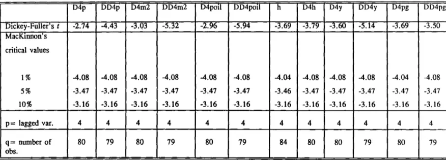
In estimating the inflation equation we experimented with the error correction model and with the partial adjustment model, before choosing the more simple specification given by eq.(3) in which ali the variables are defined as accelerations. We used accelerations rather than rates of changes because the latter are not stationary. The Dickey-Fuller tests for the existence ofUnit Roots presented in Table 3 show that all variables expressed as accelerations are stationary while not ali variables expressed as frrst differences are stationary. On the other hand there is no evidence that the variables expressed as frrst differences are cointegrated.
Our data bank starts in 1970.1 and ends in 1992.1. However, because of the definitions of the variables (accelerations of frrst difference changes with respect to the same quarter of the previous year) and because of long lags for the explanatory variables, 10 observation are lost.
I D4p DD4p D4m2 I I Dlckey-Fuller's t -2.74 -4.43 -3.03 MacKmDoo's criticai values 1% -4.08 -4.08 -4.08 5% -3.47 -3.47 -3.47 10% -3.16 -3.16 -3.16 P = lagged var. 4 4 4 q= number of 80 79 80 obs.
Table 3 Italy: Dickey-Fuller Test for the Existence of Unit Roots
DD4m2 D4pOlI DD4pOlI h D4h D4y DD4y
-5.32 -2.96 -5.94 -3.69 -3.79 -3.60 -5.14 -4.08 -4.08 -4.08 -4.04 -4.08 -4.08 -4.08 -3.47 -3.47 -3.47 -3.46 -3.47 -3.47 -3.47 -3.16 -3.16 -3.16 -3.16 -3.16 -3.16 -3.16 4 4 4 4 4 4 4 79 80 79 84 80 80 79 D4pg , DD4pg , D4tys ' DD4tys " -3.69 -3.50 -3.51 -6.06 -4.04 -4.08 -4.08 -4.00 -3.47 -3.47 -3.47 -3.47 -3.16 -3.16 -3.16 -3.16 4 4 4 4 80 79 80 79
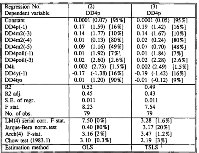
Table 4 contains the estimates of eq.(3) for consumer prices 14 . Among the supply 'shock variables we have added also a variable reflecting tax increases: the seasonally adjusted ratio of total tax revenues to GDP (tys). To be more precise, this variable is introduced as follows in the regressions:
The reason for the inclusion of this tax variable is that tax increases were very high in ltaly during the sample period. Ali other variables are defined in the same way.
Table 4 - Italy: estimates of the inflation equation, consumer prices, quarterley data, 1972.3 - 1992.2 RegresslOn No. (2) (3) Dependent variable DD4p DD4p Constant 0.0001 (0.07) [95%] 0.0001 (0.05) [95 %] DD4p(-1) 0.17 (1.59) [16%] 0.19 (1.42) [16%] DD4m2(-3) 0.14 (1.77) [10%] 0.14 (1.67) [10%] DD4m2(-4) 0.01 (0.13) [80 %] 0.02 (0.24) [80%] DD4m2(-5) 0.09 (1.16) [49%] 0.07 (0.70) [48%] DD4poi1(-1) 0.01 (1.92) [7%] 0.01 (1.84) [7%] DD4poi1( -3) 0.02 (2.60) [2.6%] 0.02 (2.28) [2.6%] D4h 0.002 (2.73) [1.5%] 0.002 (2.49) [1.5%] DD4y(-1) -0.17 (-1.38) [16%] -0.19 (-1.42) [16%] DD4tys 0.01 (1.20) [90%] -0.01 (-0.12) [9%] R2 0.52 0.49 R2 adj. 0.45 0.43 S.E. of regr. 0.011 0.011 F stat. 8.23 7.54 No. of obs. 79 79
LM(4) serial corro F-stat. 7.50 [0%] 3.28 [1.6%]
Jarque-Bera norm. test 0.40 [80%] 3.17 [20%]
Arch(4) F-stat. 3.16 [2%] 3.47 [1.2%]
Chow test (1983.1) 3.10 [0.3%] 2.19 [3%]
Estimation method OLS TSLS 1.
Note: the numbers in parenthesis are t-statistics and significance leveis respectively.
1 Instrument list: Constant, and DD4m2, DD4poil, D4h, DD4y, g ,and cays lagged variables.
14For interesting econometric studies of the determinants of inflatioD for ltaly see Micossi and Papi (1993) and Favero and Spinelli (1992).
Regressions (2) and (3) of Table 4 are the most satisfactory we could estimate for co~sumer
prices for the whole period. Once it was decided for the reasons mentioned above to estimate eq. (3) in terms of accelerations the starting point of the estimation was a general version of eq. (3) with all explanatory variables lagged three quarters. After simplifying the general specification using Hendry's methodology we obtained the estimates presented in Table 4. The interest rate has been removed frem the list if explanatory variables because its inclusion leads to parameter instability. Regr. (2) is estimated by OLS and reg r. (3) by Two-Stage-Least-Squares (TSLS). The second technique was used to take into account the fact that some explanatory variables may be endogenous. The results are breadly the same as in the OLS estimation.
Significant explanatory variables are lagged money, the bussiness cycle and the oil price. The regressions do not pass ali the standard statistical tests. For instance the residuais of regression (2) pass the test of normality but they are serially correlated and heteroskedastic. The same holds for regr. (3). In addition the Cusum of squares test indicates a structural break of the function at the 5 %
levei in the second quarter of 1983. Fig. 3 shows that the Cusum statistics cresses or is very close to the upper bound of the 5 % significance levei line 15. To verify the structural break, we performed a break-point Chow test using 1983.1 to partition the data set. The test (Table 3) validates the structural break hypothesis of the data set as the F-statistics is significantly large (significance levei of only 0.3 %). Ali the stability tests performed point to the second quarter of 1983, including the recursive parameters estimates performed with a similar equation and described in Tullio and Ronci (1994).
These largely unsatisfatory results are caused by the hybrid nature of the sample period chosen for estimation. We have flexible exchange rates since March 1973 and then starting in March 1979 the ERM of the EMS. During the ERM period German inflation which is not included in the regressions should be expected to increase its influence on ltalian inflation and ltalian money to loose gradually its importance as the system becomes more credible. The constant term should also be expected to fali as the ERM becomes more credible.
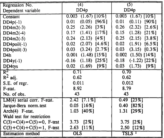
Once we have established the partitioning of the data set we estimated again equation (3) for the 1972.3-1983.1 period (Table 5, regressions 4 and 5) in which exchange rates were flexible. The results seem to support generally our inflation equation specification. The length of the lags for money and oil are very plausible. Real GDP growth reduces inflation by increasing the real demand for money, as expected. The business cycle is also contributing to some extent to explain ltalian inflation, along with taxes. The coefficients of lagged accelerations of inflation never tum out to be significantly different from zero, suggesting that there was no "inertia" in the inflationary process, despite the strong indexation of wages during most of the period. The Cusum of squares test (Fig. 4) is well behaved and statistical tests for serial correlation, normality and heterokedasticity suggest no serious specification preblems.
Table 5 Italy: Inflation Equation, consumer prices, flexible exchange rate period,1972.3-1983.1 Regression No. (4) (5) Dependent variable DD4p DD4p Constant 0.003 (1.67) [10%] 0.003 (1.67) [10%] DD4p(-l) 0.01 (0.05) [96%] 0.01 (0.11) [90%] DD4m2(-3) 0.25 (2.26) [3%] 0.26 (2.32) [2.6%] DD4m2(-4) 0.17 (1.41) [17%] 0.15 (1.28) [21 %] DD4m2(-5) 0.24 (2.13) [4%] 0.25 (2.15) [3.8%] DD4poil(-1) 0.02 (2.07) [4.6%] 0.02 (1.91) [6.5 %] DD4poil(-3) 0.03 (3.24) [2.7%] 0.03 (3.15) [0.3 %] D4h 0.001 (1.48) [15 %] 0.002 (1.50) [14%] DD4y(-1) -0.16 (1.18) [25 %] -0.18 (-1.22) [22 %] DP4tys 0.02 (1.69) [9%] 0.03 (1.73) [9%] R"" 0.71 0.70 R2 adj. 0.62 0.62 S.E. of regr. 0.011 0.012 F-stat. 8.92 8.79 No. of obs. 43 43
LM(4) senal corro F-stat. 2.42 [7.1%] 0.49 [23%]
Jarque-Bera norm.test 0.05 [16%] 0.40 [82%]
Arch(4) F-stat. 1.03 [40%] 1.31 [29%]
Wald test for restriction
C(3)=C(4)=C(5)=0, F-test 3.73 [2%] 3.75 [2%]
C(3)+C(4)+C(5)=I, F-test 2.63 [11 %] 2.50 [12%]
Estimation method OLS TSLS I
Note: numbers in parenthesis are t-statistics and significance leveI, respectively. 1 Instrument list: Constant, and DD4m2, DD4poil, D4h, DD4y, g" and cays lagged variables
In addition, the Wald tests for the null-hypothesis that the sum of the coefficients of money is not significantly different trom one cannot be rejected at the one percent significance leveI for regresions (4) and (5).
We performed an out of sample focecast with regr. (4) starting trom 1983.2. It turns out that this regression tends to strongly overpredict inflation after 1983.1. The cumulated error of the forecast amounts to about 17 percent at the end of the sample period, which implies that the model overestimates inflation on average by about 0.5 percentage points per quarter or about 2 percentage points per year, which is a substantial error. This confrrms the conclusions drawn above that after 1983.1 there was a structural break in the equation determining inflation in Ita1y and that this break must have been caused by the increased credibility of the ERM and the increased importance of German inflation in determining the ltalian one. 16
If the quantity theory breaks down as an explanation of ltalian inflation after 1983.1; what explains it then? Under perfectly fixed exchange rates, goods arbitrage is expected to bring about a tendency towards equalization ofprice dynamics between Italy and Germany; in terms ofaccelarations of inflation we have in the long run:
Where b
o
=
O and b 1=
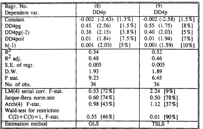
1. The estimates of equation (5) for consumer prices with the addition of lags for DD4Pg,
oil shocks (because they may affect ltaly differently than Germany) and the business cycle are reported for the credible ERM period (1983.2-1992.1) in Table 6. The results suggest strongly the correctness of our specification. The Cusum of squares test (Fig. 5) shows a well behaved pattern, although at the beginning of the period the statistics is close to the upper bound of the 5 % significance leveI. In the credible ERM money plays no role any more. On1y German inflation, the business cycle and to some extent oil matter. In addition, a Wald test for the null hypothesis that the sum of the two coefficients of German inflation is equal to one is accepted at the 1 % significance levei.Table 6 Italy: Inflation Equation! fixed exchange rate period, 1983.2-1992.1 Regr. No. (8) (9) Dependem var. DD4p DD4p Constam -0.002 (-2.63) [1.3%] -0.002 (-2.58) [1.5 %] DD4pg 0.45 (2.56) [1.5 %] 0.55 (1.75) [8%] DD4pg(-2) 0.38 (2.15) [3.8 %] 0.40 (2.03) [5%] DD4poil 0.01 (1.84) [7.5 %] 0.01 (1.94) [7%] h(-I) 0.001 (2.03) [5%] 0.001 (1.59) [10%] Rk 0.54 0.52 R2 adj. 0.48 0.46 S.E. of regr. 0.005 0.005 D.W. 1.93 1.89 F stat. 9.23 6.45 No. of obs. 36 36
LM(4) serial corr. F-stat. 0.53 [72 %] 2.24 [9%]
Jarque-Bera norm. test 0.60 [74%] 0.50 [78%]
Arch(4) F-stat. 0.98 [43%] 1.12 [37%]
Wald-test for restriction
C(2)+C(3)= 1, F-stat. 0.55 [46%] 0.01 [~%]
Estimation method OLS TSLS J.
Note: numbers in parenthesis are t-statistics and significance leveis, respectively. 1 Instrument list: Constant and DD4pg, DD4poil, and h Iagged variables.
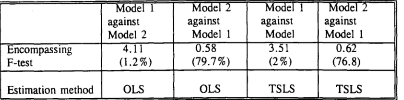
Finally, we tested Model 1 (equation 3) against Model 2 (equation 5) for the 1983.2-1992.1 period. We performed non-nested encompassing F-tests and found that Model 2 is clearly superior to Model 1 in the period of flXed exchange rates 17 (Table 7).
Table 7: Ital)': Test for Non-Nested Regression Models for Inflation, 1983.2-1992.1
Model 1 Model2 Model 1 Model2
against against against against
Model2 Model 1 Model Model 1
Encompassing 4.11 0.58 3.51 0.62
F-test (1.2%) (79.7%) (2%) (76.8)
Estimation method OLS OLS TSLS TSLS
Note: Regressors of Model 1 are DD4p(-1), DD4m2(-3), DD4m2(-4), DD4m2(-5), DD4poil(-l), DD4poil(-3), D4h, DD4y(-1), and DD4tys; and Regressors of Model 2 are DD4pg, DD4pg(-2), DD4poil, and h(-l).
5. Summary and conclusions
The main conclusions of this paper are the following:
1. The quantity theory of money explains very well ltalian inflation during the flexible exchange rate period which goes from 1973 to 1983, despite the creation of the EMS in March 1979. We did not find support for the so-called inertia-hypothesis of inflation, despite the strong indexation of ltalian wages.
2. ltalian anti-inflation policies made large gains in credibility in 1983, when a significant structural break occurred in the inflation equation.
3. Increased Central Bank autonomy and the development of the secondary market for governrnent debt were crucial in contibuting to bring ltalian inflation down. They went hand in hand with the increased credibility of the ERM-exchange rate constraint during the 1980's. For this reason it is difficult to separate the effect of changes in the monetary constitution on inflation from the effects of the ERM. We have tended to attribute the 1983 structural break in the inflation equation mainly to the increased credibility of the ERM
after the French U-turn, although without the previous changes in the monetary
constitution the break would probably not have been possible. The evidence presented indicates that changes in the actual behaviour of the Bank of ltaly were not highly correlated with changes in the monetary constitution.
4. The estimates of the reaction function suggest also that the ltalian Central Bank had a very stable behaviour, except for the break in the degree of monetary financing of the government budget deficit in 1977, although it systematically tended to destabilize the business cycle by giving a high priority to the monetary financing of aggregate demand booms up to the point where the externaI (current account) constraint was hit. If the Bank of ltaly continued to behave after January 1st 1994 (when it gained full autonomy) according to the reaction function estimated up to the beginning of 1992, the inflation outlook in ltaly does not look very rosy, because the rate of growth of money in the reaction function estimated does not show a negative reaction to inflation; it shows instead a positive one to the business cycle which in early 1995 was in full recovery at a time
when the externai constraint was not binding (as the current account shows a large surplus) . and casual observation suggests that the Bank did not react to depreciations of the lira with respect to the O M.
5. As to the fiscal dominance hypothesis we find that it is largely confirmed for the period up to the end of 1977. A significant reduction of the link between fiscal deficits and monetary growth occurred at the end of 1977, a change which was "institutionalized" only four and a half year later with the July 1981 divorce and further strenghened in 1992 and 1994.
6. There is an active debate in many countries about the usefulness of inflation targeting by the Central Bank, which consists in fixing and announcing an inflation target and in making a serious committment to achieve it. At the time of writing the Banca d'Italia does not announce an inflation target. lt prefers instead to hide, as it has frequently done in the past, behind the irresponsible Italian fiscal policy, the alleged cause of all Italian evils. However, as every student of economics knows, inflation depends also on monetary policy; in the medium to long run it depends much more on monetary than on fiscal policy. The Banca d'Italia has now full autonomy and in addition exchange rates are again perfectly flexible (since September 1992), a fact which enhances the degree of independence of monetary policy. Besides, since 1992, fiscal policy has become a lot more responsible and for the first time the Governrnents are seriously trying to tackle the perverse mechanisms which cause the growth of governrnent expenditures in the long run. In fact in 1993-94, the fall in inflation from over 5 % to 3.8 %, which occurred despite the huge depreciation of the lira (about 35 % withe respect to the DM), was maily due to the very restrictive fiscal policy and to wage moderation. Now that there is no monetary anchor, the control of inflation in Italy would become more effective if the Banca d'Italia announced an inflation target and used ali its newly acquired powers to achieve it.
Appendix - Description and sources of data used
cal
=
current account in lira. Source: lnternational Financiai Statistics (lFS) of IMFcays = current account surplus/Y, seasonally adjusted.
DEF = Treasury financing requirement. Source: Banca d'ltalia (BI)
D77 = dummy = 1 from 1970.1 to 1977.4
EDM = official exchange rate of the lira with the Deutsche Mark. Source: IFS
g = seasonally adjusted DEF/Y
h = (real GDP - real YT)/real YT
i = nominal interest rate on private medium term bonds; average for last month in quarter, in percent per year.
Mo = monetary base, end of period. Source B.I.
M2 = money stock (currency plus bank deposits), end of period. Source: BI.
P = consumer price index, last month of quarter. Source: ISTAT.
P2 = wholesale price index, last month of quarter. Source: ISTAT
PD1 - total public debt. Source: B.1.
PD3 = total public debt held by the Banca d'Italia. Source: B.I.
PG = German consumer price index, last month of quarter. Source: IFS, line 64.
POIL = price of oi!, in US dollars converted into liras at the official lira US-$ exchange rate
S = official exchange rate of lira with the US dollar. Source: IFS
tys = ratio of total govemment revenues to nominal GDP, seasonally adjusted
separately from 1970.1 to 1981.4 and 1982.1 to 1992.1
Y = GDP real. Source: ISTAT.
YN = GDP nominal. Source: ISTAT.
YT = trend of real GDP computed separately for the 1970's and the 1980's by
,l'~' '6F~\ MAQro
RENRtOt
1f F;;;~: .. ·i::1regressing Y 011 a constant and time
TGR
=
governrnent revenues.Dx
=
first difference operator: lower case letters indicate logs of ratios or variables (like g and h above). Ali first difference for ltaly are defined with respect to the same quarter of the previous year; thusD4Xt
=
log xt - log Xt-4'References
Agenor, Pierre-Richard and Tylor, Mark P.
Testing for Credibility Effects.
IMF Working Paper, 1991.Banerjee, Anindya, luan Dolano, lohn Galbraith, and David Hendry
Co-Integration, Error
Correetion, and the Eeonometrie Analysis of Non-Stationary Data.
Oxford University Press, 1993.Burdekin, Richard C.K. and Laney, Leroy O. Fiscal Policymaking and the Central Bank Institutional Constraint,
Kyklos,
VoI. 41, 1988, 647-662.De long Eelke, "The determiants of inflationary expectations in the EMS", paper prepared for the EEC SPES Projet No. CT91-0053, 1994, forhcoming as Chapter 10 of
Injlation
and
wage behaviour in the EMS.
Paul De Grauwe, Stefano Micossi and Giuseppe Tullio(eds.), Oxford University Press, Oxford.
Favero Carlo and Spinelli Franco " Deficits , Money Growth and Inflation in Italy: 1865-1990", Working paper No. 279, University of London, October, 1992.
Ghosh, Sukesh K.
Eeonometries: Theory
andApplieations.
Prentice Hall, 1991.Goodman, lohn B.
Monetary Sovereignity: The Polities of Central Banldng in Westem
Europe.
Ithaca and London: ComelI University Press, 1992.Hall, Robert, lack lohston, and David Lilien
MieroTSP User's Manual: Version 7.0.
Irvine,· California: Quantitative Micro Software, 1990.Harvey, A.C.
The Eeonometrie Analysis of Time Series.
Philip AlIan, 1985.Masera Rainer S.
Disavanzo Pubblieo e Vineolo di BiIando.
Edizioni di Comunità a cura delIaBanca Commerciale Italiana, Milano, 1979.
Micossi Stefano and Papi Laura "The growth in the public sector and Italian inflation in the 1970's and 1980's paper prepared for the EEC-SPES Project CT91-0053 1994,
forhcoming as Chapter 4 of
Inflation and wage behaviour in the EMS.
Paul De Grauwe,Passacantando Franco. "Monetary Reforms and Monetary Policy in ltaly from 1979 to 1994", paper presented at the FGV -Conference on the Search for Monetary Stability, September 1 1994, Rio de Janeiro,
Spinelli, Franco and Fratianni, Michele Storia Monetaria d'/talia. Milan: Amoldo
Mondadori Editore, 1991.
Spinelli Franco, SuUa politica monetan'a italiana e intemazionale. Franco Angeli, Milano,
1986.
Tullio Giuseppe and Ronci Mareio, "Macroeconomic Poliey and eredibility: a comparative study of the factors affecting Brazilian and ltalian inflation after 1970. ", EPGE Working paper No. 247, Fundacao Getulio Vargas, Rio de Janeiro, October 1994 and Luiss University Working paper No.54, Rome, December 1995.
Tullio G., "Inflation and Currency Depreciation in Germany 1920-23: a dynamie model of prices and the exchange rate", Joumal of Money, Credit and Banking, forthcoming, May 1995.
Visco, Ignazio, "Inflation, inflation targeting and monetary poliey: notes for diseussion on the ltalian experience", paper presented at the CEPR Inflation Targets Workshop, Milan, Nov. 1994.
~---~125
100
75
50
25
70
72
74
76
78
80
82
84
86
88
90
1-
Real interest rate ---
PublicDebtl
."
g.
-2.5
-5.0
~-
o-7.5
-...
G) Q-10.0
o--
.g
-12.5
Q..-15.0
-17.5
(as percentage of GDP )
70
72
74
76
78
80
82
84
86
88
90
1-
Public Deficit --- Public Debtl125
100
75
50
25
."g.
--
(') I:' (p ~•
CUSUM
of Squ ares
1.25~---~
1.00
0.75
0.50
0.25
",,-"
,J.'
. ' ".'
.'
. ',.
0.00~---.~'·---4---~1976
1978
1980
1982
1984 1986
1988
1990
CUSUM
of Squ ares
1975
1976
1977
1978
1979
1980
1981
1982
.
Fig. 5 Italy: Inflation Equation (ERM), 1982-1992.1
CUSUM
of Squ ares
1.50~---~
1.25
1.00
0.75
0.50
0.25
1985
1986
1987
1988
1989
1990
1991
'4'
h'~Gt
UL10
/ ('~ ~~ / ~~ ..,.~ "~<ç\
,(»' (fi 1'-1...G~8L10TECA
M':'RIO HW::ICUE SIMONSEN
..
000088368
1/11111111111111111111111111111111111
l'I'.Cham. P/EPGE SPE R236c
Autor: Ronei, Mareio Valerio.
Título: Central Bank autonollly. the cxchangc rale
08~06X
1/11111111111111111111111111111111111111 51508