A FULLY ADAPTIVE FRONT-TRACKING METHOD FOR
THE SIMULATION OF 3D TWO-PHASE FLOWS
UNIVERSIDADE FEDERAL DE UBERL ˆ
ANDIA
FACULDADE DE ENGENHARIA MEC ˆ
ANICA
A FULLY ADAPTIVE FRONT TRACKING METHOD FOR THE
SIMULATION OF 3D TWO-PHASE FLOWS
Tese apresentada ao Programa de P´os-graduac¸˜ao em Engenharia Mecˆanica da Universidade Federal de Uberlˆandia, como parte dos requisitos para a obtenc¸˜ao do t´ıtulo deDOUTOR EM ENGENHARIA MEC ˆANICA.
´
Area de concentrac¸˜ao: Transferˆencia de Calor e Mecˆanica dos Fluidos.
Orientador: Prof. Dr. Aristeu da Silveira Neto Co-Orientador: Prof. Alexandre M. Roma, Ph.D.
Pivello, M´arcio Ricardo, 1975 –
A fully adaptive front-tracking method for the simulation of 3D two-phase flows / M´arcio Ricardo Pivello; orientador: Aristeu da Silveira Neto; co-orientador: Alexandre M. Roma – Uberlˆandia, 2012.
132 p.:il.
Tese (Doutorado) – Universidade Federal de Uberlˆandia, Programa de P´os-graduac¸˜ao em Engenharia Mecˆanica.
I would like to express my sincere gratitude to my advisors, Professors Aristeu and Alexandre, for their invaluable guidance and great patience;
To Ricardo Serfaty, for the useful suggestions;
To all my friends at MFLab, for their support, especially Millena and Rafael, for their active and steady help on the development of this work;
To professor Antˆonio Castelo Filho, for the support on the implementation of the TSUR-3D algo-rithm,
To Thiago Pinheiro de Macedo, for providing the (skilfully implemented) computational code that became the basis for the implementation of the indicator function;
To Wellington Carlos de Jesus, for the fundamental discussions about memory leaks;
To my wife, Tatiana, for her love and comprehension during all these years;
To my parents, Olivio and Neuza, and my sisters, Sabrina and Luciana, for their love and support;
To the Federal University of Uberlˆandia and the School of Mechanical Engineering, for providing the computational support for the fulfilling of this work;
PIVELLO, M.R., A fully adaptive front-tracking method for the simulation of 3D two-phase flows. 2012. 132 f. PhD Thesis, Universidade Federal de Uberlˆandia, Uberlˆandia, Brasil.
ABSTRACT
This thesis presents a computational framework for simulating three-dimensional two-phase flows based on adaptive strategies for space and time discretization. The method is based on the front-tracking method of Unverdi and Tryggvason (1992), and the discretization of the Eulerian domain is based on the SAMR strategy of Berger and Colella (1989). The time integration algorithm is based on the IMEX scheme, and the time step is calculated based on CFL criteria. The imple-mentation of the Lagrangian framework relied on the GNU Triangulated Library (GTS), which provides a complete data structure and supporting functions for data access, remeshing tools and data output. The memoryless simplification algorithm of Lindstrom and Turk (1998) is used for surface remeshing, preserving the volume and shape of the interface. Nevertheless, additional tools for volume recovery were implemented, motivated by the non-conservative behaviour of the advec-tion of the Lagrangian interface. This process may also induce some non-physical undulaadvec-tions on the Lagrangian interface, which was circumvented with the implementation of the TSUR-3D algo-rithm of Sousa et al. (2004). The methodology was applied to a series of rising bubble simulations, in which a single bubble rises in an initially quiescent liquid, and validated against experimental results (BHAGA; WEBER, 1981). The validation process consisted in comparing the terminal shape and Reynolds number, as well as the topology of the streamlines downstream of the bubble. Finally, the algorithm was applied to the simulation of two cases of bubbles rising in the wobbling regime, which is characterized by the continuous change in the bubble shape and complex patterns of vortex shedding. The use of adaptive mesh refinement strategies led to physically insightful results, which would not be possible in a serial code with a uniform mesh.
PIVELLO, M.R., Um m´etodo front-tracking completamente adaptativo para a simulac¸˜ao de escoamentos tridimensionais bif´asicos. 2012. 132 f. Tese de Doutorado, Universidade Federal
de Uberlˆandia, Uberlˆandia, Brasil.
RESUMO
Nesta tese apresenta-se um algoritmo para a simulac¸˜ao de escoamentos tridimensionais bif´asicos, aliando-se o m´etodo defront-trackingde Unverdi and Tryggvason (1992) a estrat´egias adaptativas para a discretizac¸˜ao espacial e temporal. A discretizac¸˜ao do dom´ınio Euleriano utiliza a metodolo-gia SAMR (BERGER; COLELLA, 1989), enquanto o algoritmo de integrac¸˜ao temporal utiliza o esquema IMEX com c´alculo do passo de tempo com base em crit´erios CFL. A implementac¸˜ao da estrutura computacional Lagrangiana baseou-se na biblioteca GNU Triangulated Library (GTS), que fornece estrutura de dados completa e um algoritmo de remalhagem baseado t´ecnica memory-less simplification algorithm, que garante preservac¸˜ao da forma e do volume da geometria
(LIND-STROM; TURK, 1998). Ainda assim, ferramentas adicionais para recuperac¸˜ao de volume foram implementadas, devido ao comportamento n˜ao conservativo da advecc¸˜ao da interface Lagrangiana. Este processo tamb´em pode induzir ondulac¸˜oes n˜ao f´ısicas na interface, o que foi contornado com a implementac¸˜ao do algoritmo TSUR-3D de Sousa et al. (2004). A metodologia proposta foi apli-cada a uma s´erie de simulac¸˜oes nas quais uma ´unica bolha ascende em um l´ıquido inicialmente em repouso. Os resultados foram comparados com dados experimentais de Bhaga e Weber (1981). A validac¸˜ao foi feita comparando-se o n´umero de Reynolds e a forma da bolha em regime terminal, bem como a topologia das linhas de corrente. Finalmente, o algoritmo foi aplicado `a simulac¸˜ao de dois casos dewobbling, regime caracterizado pela mudanc¸a cont´ınua da forma da bolha e por padr˜oes complexos de liberac¸˜ao de v´ortices. O uso de malhas adaptativas forneceu detalhes do escoamento que dificilmente seriam obtidos em um c´odigo serial com refinamento uniforme, pois demandaria uma resoluc¸˜ao muito alta da malha.
Palavras chave: Front Tracking, refinamento adaptativo de malhas, preservac¸˜ao de volume,
1.1 Flow patterns for a vertical pipe gas-liquid flow(MUDDE, 2005). . . p. 25
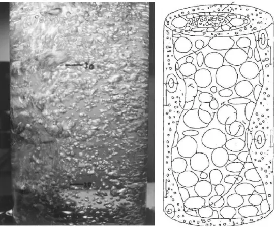
1.2 An example of bubble column. Left: a laboratory-scale bubble column (WAR-SITO et al., 1999) in the heterogeneous regime. Right: A schematic
representa-tion of the flow pattern (PORTELA; OLIEMANS, 2006). . . p. 26
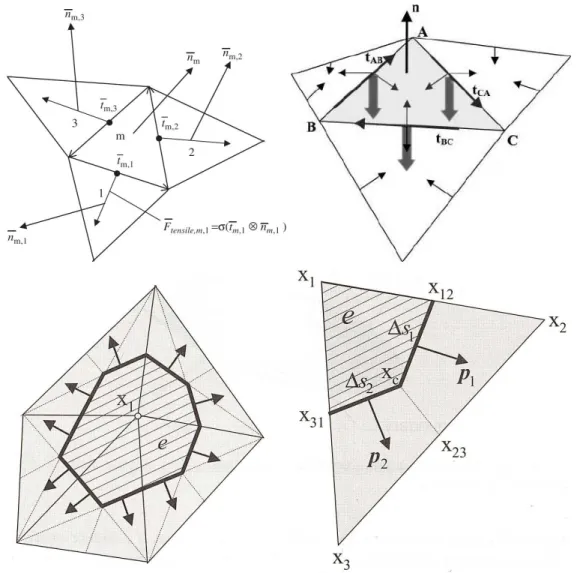
2.1 Three different ways to calculate the interface tension force on a surface element. On the top, using the mesh element as the integration element (left: Deen, Anna-land and Kuipers (2004), right, Singh and Shyy (2007)). At the bottom, building the integration elements around the mesh vertexes, based on the centroid of the mesh elements sharing the vertex, proposed by Tryggvason, Scardovelli and
Za-leski (2011). . . p. 37
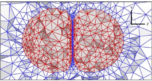
2.2 An example of the mesh adaptation in the MMIT method in the simulation of
the merging of two droplets (QUAN; LOU; SCHMIDT, 2009). . . p. 39
2.3 Mesh grading applied to a cartesian grid (left) (DURBIN; IACCARINO, 2002)
and to a multiblock grid (right) (CAGNONE et al., 2011). . . p. 39
2.4 An example of Chimera grid in the simulation of the flow around a helicopter. Left: the mesh around the entire helicopter. Right: a detail of the mesh around
the rotor (RENAUD; COSTES; PRON, 2012). . . p. 40
2.5 An octree grid used in the simulation of the flow around a boat (POPINET, 2003). p. 41
2.6 An example of block structured adaptive mesh refinement. The vortex shedding behind a rising bubble is refined based on the gradient of the vorticity. In the
3.1 A closed curveCand the regions in which the closest points not inCare orthog-onal to an element of the mesh. Left: regions delimited by the outer normals.
Right: regions delimited by the inner normals (MAUCH, 2003). . . p. 47
3.2 The bounding regions are determined by the normals of neighbour elements sharing a vertex. Left: normals point outsideC. Right: normals point insideC
(MAUCH, 2003). . . p. 47
3.3 Delimiting prism for the shortest distance from a point in space and the face of
an element of a mesh. . . p. 48
3.4 CPT Bounding regions for edges and vertices (AZEREDO, 2007). . . p. 49
3.5 An example of block structured adaptive mesh refinement properly nested
(VIL-LAR, 2007). . . p. 55
3.6 An example of block structured adaptive mesh refinement violating the nesting rules: the fine block in grid (a) does not lie on vertices of the coarse level block and the block in the finest level in grid (b) touches the boundary of a block in
the next coarse level which is not part of the domain boundary (VILLAR, 2007). p. 55
3.7 Example of adaptive mesh refinement using based on the vorticity magnitude. . p. 56
3.8 The volume change after advecting the interface is assumed to be due to an
expansion/contraction of the geometry in the normal direction. . . p. 58
3.9 The prism conceptually formed by a typical interface element and the expansion
gaphafter the interface advection. . . p. 58
3.10 Computing a normal vector at vertex v. For each element iconnected to v, ni is the normal of this element,ei1andei2 are the edges of the element which are
used for computingniandαiis the angle betweenei1andei2. . . p. 59
3.11 Wrinkles at the rear of rising bubbles. Left: Spherical cap,Eo=40,M=0.056. Simulation carried out in the present Work. Right: Intermediate wobbling + spherical cap,Eo=10.0,M=9.71·10−12 (ANNALAND; DEEN; KUIPERS,
3.12 Undulation Removal procedure: repositioning a generic edge e(SOUSA et al.,
2004). . . p. 61
3.13 Edge collapse in the Memoryless Simplification algorithm of Lindstrom and
Turk (1998). . . p. 64
3.14 Constraints for calculating the coordinates of a new vertex in the Memoryless
Simplification algorithm of Lindstrom and Turk (1998). . . p. 65
4.1 Static grid with one refinement level used on the convergence rate analysis. . . p. 70
4.2 Surface mesh of a unit cube before and after mesh coarsening. . . p. 73
4.3 Surface mesh of a unit sphere before and after mesh coarsening. . . p. 73
4.4 Eulerian cells flagged by the indicator function for a spherical geometry. . . p. 74
4.5 Deformation of a spherical surface when subjected to the analytical velocity field
given by Eq. (4.11). Snapshots taken att=0,t= T4,t =T2,t= 34T et=T . . . p. 75
4.6 The influence of velocity interpolation and surface remeshing on the
preserva-tion of the initial interface volume. . . p. 77
4.7 The influence of the volume recovery algorithm on the preservation of the initial
interface volume. . . p. 78
4.8 Clift Diagram (CLIFT; GRACE; WEBER, 1978) and the cases simulated in this
work (bubble shapes shown in black). . . p. 81
4.9 A-series: Terminal Reynolds number depending on the geometric intervention
applied. Reference Reynolds number: Re=20.6. . . p. 82
4.10 A-series: Bubble shape and relative position at the beginning and at the end of the simulation, depending on the geometric intervention applied. From left to
right: cases A1, A2, A3 and A4. . . p. 83
4.11 A-series: Temporal evolution of wrinkles when no smoothing procedure is
4.12 Bubble shape at the end of the simulation. Top: no geometric intervention.
Bottom: volume recovery and wrinkle removal. . . p. 84
4.13 A-series: Streamlines inside and at the rear of the bubble. Top: no geometric
intervention. Bottom: volume recovery and wrinkle removal. . . p. 85
4.14 A-series. Influence of the domain size on the relative position at the end of the
simulation. Left to right: 4φ, 6φ, 8φ, 10φ. . . p. 86
4.15 A-series. Influence of the domain size on the bubble Re profile. Reference
Reynolds numberRe=20.6. . . p. 86
4.16 Lagrangian mesh resolution. From top to bottom: λξ =1,λξ =2 andλξ =4 . p. 87
4.17 Influence of the Lagrangian mesh resolution on the bubble Reynolds profile. . . p. 88
4.18 Cross section of the terminal bubble shape depending on the Lagrangian edge length, for a fixed Eulerian grid size and varying Lagrangian characteristic length.
: λξ =1. : λξ =2. △:λξ =4. . . p. 88
4.19 Rising bubble. Influence of the density ratio on the ascending velocity. . . p. 89
4.20 Reynolds profile for a spherical rising bubble at Eo=8.67 and M=711.
Experi-mental terminal Re = 0.078 according to Bhaga and Weber (1981). . . p. 90
4.21 Effect of the density ratio on the trajectory of a wobbling bubble. Green bubble: density ratio = 10. Grey bubble: density ratio = 100. On the right: The straight
line corresponds to ratio = 10. . . p. 91
4.22 Streamlines showing a toroidal vortex inside the bubble and another vortex
downstream. Density ratioλρ =10. . . p. 91
4.23 Patches of the finest level of the adaptive mesh. Refinement was performed based on the vorticity magnitude, as well as on the position of the Lagrangian
4.24 A simplified schematic drawing of the experimental apparatus utilized by Bhaga and Weber (1981), showing the bubble release mechanism: 1, test column; 3,
dumping cup; 4, air inlet; 5, inverted funnel; 16, rising bubble. . . p. 96
4.25 Influence of the initial shape on the evolution of the bubble shape. Eo=116,
M=41.1,Re=7.16. . . p. 97
4.26 Influence of the initial shape on the Reynolds profile. Eo=116, M =41.1,
Re=7.16. . . p. 97
4.27 Eo =116, M =8.6×10⁻⁴, Re=151. Influence of the initial shape on the
evolution of the bubble shape. . . p. 98
4.28 Eo =116, M =8.6×10⁻⁴, Re=151. Influence of the initial shape on the
Reynolds number profile. . . p. 98
4.29 Wobbling bubble, Eo=10 andM=9.78×10⁻⁸. Centroid path shown in 3D. The zigzag path can be seen in the beginning of the flow, and then the transition
to spiral . . . p. 99
4.30 Wobbling bubble,Eo=10 andM=9.78×10⁻⁸. Velocity profile of the bubble
centroid. . . p. 100
4.31 Wobbling bubble, Eo=10 and M= 9.78×10⁻⁸. Time evolution of vortex
shedding. Iso-q = 5000. . . p. 101
4.32 Wobbling bubble, Eo=10 andM=9.78×10⁻⁸. Example of grid adaptation
based on the vorticity gradient. . . p. 101
4.33 Wobbling bubble,Eo=10 andM=9.78×10⁻⁸. Velocity field inside the
bub-ble. Planes warped by the velocity vector. . . p. 102
4.34 Wobbling. Eo =3.6, M =2.5×10⁻¹¹. Q-criterion = 5000 and streamlines.
4.35 Wobbling. Eo=3.6, M=2.5×10⁻¹¹. Top: Q-criterion Q=5000 in green, z-vorticity in redωZ = +50 and blue ωZ =−50. Bottom: bubble shape at the
respective time instants. . . p. 104
4.36 Wobbling. Eo=3.6,M=2.5×10⁻¹¹. Iso surfaces of the z-component of the
vorticity. Red=+50, blue = -50. . . p. 105
4.37 Time evolution of the vortex shedding behind the bubble, showing the varicose mode. Left: Iso-surfaces of the vorticity magnitude. Center: Iso-surface of the
Q-criterion. Right: bubble shape. . . p. 106
4.38 Time evolution of the vortex shedding behind the bubble, showing the varicose
mode (cont.). . . p. 107
4.39 Overall time cost of each task group, when taking into account the entire sim-ulation. Pressure: 75.930%; velocity: 6.296%; writing restart files: 0.006%; Lagrangian operations: 12.468%, AMR operations: 5.145%, writing output for
post-processing:0.005%, others: 0.069%. . . p. 108
4.40 Time cost of each task group, when taking into account only the time steps in which the Eulerian domain was remeshed. Pressure: 17.191%; velocity: 1.500%; writing restart files: 0.633%; Lagrangian operations: 2.933%, AMR
operations: 77.692%, writing output for post-processing:0.034%, others: 0.017%. p. 109
4.41 Time cost of each task of the Lagrangian group, when taking into account the entire simulation. Surface remesh: 39.986%, transferring information from IB-GTS to AMR3D:2.511; Lagrangian maps: 7.214%, Velocity Interpolation: 0.000%, spreading the interface force on the Eulerian grid: 18.110%, TSUR3D:
A.1 The coalescence algorithm applied to two spheres. The main sequence of the algorithm is explained in the second row of the figure: the intersection between the two spheres is forced (left), then the irrelevant part of the intersection is dismissed (center) and the surfaces are taken back to their original positions, except for the vertices generated by the intersection process (right). The image on the bottom shows the necking region created by the process, overlapped with
the initial stage of the algorithm. . . p. 121
A.2 Identifying the collision of two surfaces. Only a cut of the dimpled hemisphere
is showed. . . p. 121
A.3 The merge algorithm applied to a dimpled hemisphere (only half is shown) and
a sphere. . . p. 122
A.4 An example of bubble necking in an experimental setup used for launching
bub-bles inside a tank filled with liquid (BURTON; WALDREP; TABOREK, 2005). p. 123
A.5 Breakup algorithm. The necking region (top left) is identified by number of Eu-lerian cells inside the surface (top center) and the respective surface elements are identified (top right). The centroid of the open ends of this region (bottom left) are used for computing the normal defining the cutting plane (bottom center)
and the surface is then split (bottom right). . . p. 124
B.1 Geometric data types in GTS. . . p. 126
B.2 Mesh-related data types in GTS. . . p. 126
B.3 TheGtsSurfacedata type in GTS. . . p. 126
B.4 Relationship between the data types defined in the GTS library. . . p. 127
B.5 Wrapper data types as defined inside AMR3D (left) and IB-GTS (right) for
granting AMR3D access to the geometric data of the surface. . . p. 130
B.6 A snapshot of the headers of the functions used for surface remeshing and
B.7 A snapshot of the modulegts amr3d interfaceshowing the interface for
call-ing functions for surface remeshcall-ing and calculatcall-ing the indicator function. . . . p. 131
C.1 The rise of two bubbles with different diameter. Temporal sequence is: left column, bottom to top; right column, bottom to top. Case based on (UNVERDI;
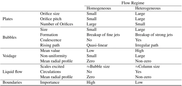
1.1 Qualitative comparison of homogeneous and heterogeneous flow regimes in
bubble columns (RUZICKA et al., 2001b). . . p. 27
2.1 Physical quantities that have influence on the terminal velocity of a rising bubble
(BHAGA, 1976). . . p. 30
4.1 Verification tests. Navier Stokes solver run with Dirichlet boundary conditions
for velocity and Neumann for the pressure. . . p. 71
4.2 Verification tests. Navier Stokes solver run with Neumann boundary conditions
for velocity and Dirichlet for the pressure. . . p. 71
4.3 Verification tests. Navier Stokes solver run with Periodic boundary conditions
for both, velocity and pressure. . . p. 72
4.4 Shear Flow. Case description for each test performed. . . p. 76
4.5 Capillarity number as a function of the Laplace number. . . p. 79
4.6 A-series: Cases description and error on the terminal Re number. Reference
Re=20.6. . . p. 82
4.7 Influence of the domain size on the terminal Reynolds number. All cases were
run withLz=16φ. ReferenceRe=20.6. . . p. 84
4.8 Influence of the Lagrangian mesh resolution on the terminal bubble Reynolds
4.9 Influence of the density ratio on the terminal Reynolds number and bubble shape. Comparison against the experimental work of Bhaga and Weber (1981).
Eo=243,M=266,Re=7.77. . . p. 89
4.10 Comparison of terminal shapes and Reynolds number reported by the reference
works (BHAGA; WEBER, 1981; HUA; LOU, 2007) and the present work. . . p. 94
4.11 Comparison of terminal shapes and Reynolds number reported by the reference works (BHAGA; WEBER, 1981; HUA; LOU, 2007) and the present work.
In-fluence of the Morton number on the terminal shapes and Reynolds number. . . p. 95
4.12 Comparison of terminal bubble wake observed in experiments (BHAGA; WE-BER, 1981) and predicted in simulation (HUA; LOU, 2007) for various Reynolds,
Morton and Eotvos numbers against results obtained in the present work. . . . p. 95
4.13 Tasks executed at each time step during the simulation, grouped according to the
purpose. . . p. 105
B.1 Some data types in C and their equivalent types in Fortran, as provided by the
|| · ||2 Euclidean norm,L2-norm. || · ||∞ Infinity norm,L∞.
(·)D Index referring to the dispersed phase
(·)C Index referring to the continuous phase
∇ Gradient operator
∇2 Laplacian operator
αi Time discretization coefficients,i=0,1,2
βi Time discretization coefficients,i=0,1
δ(x) Dirac delta function
∆ei Length of edgei, which belongs to a Lagrangian mesh
∆t Time step
∆V Volume change
∆x Grid spacing in the x-direction
∆y Grid spacing in the y-direction
∆z Grid spacing in the z-direction ε Relative error between two variables ϕ A generic property
γ Distance threshold for which the indicator function is calculated; coefficient for
deter-mining a time scheme discretization for the Navier-Stokes equations λρ Density ratio between the continuous phase and the dispersed phase
θi Time discretization coefficients,i=0,1,2
ρ density
ξL Characteristic length of the Lagrangian mesh. The average length of all edges of the
Lagrangian mesh
AS Total area of a surface or a Lagrangian mesh
AT Area of the triangleT
Nt Number of triangles in a Lagrangian mesh
C A generic 2D Lagrangian mesh Ca Capillarity number
D(x) Smooth function replacing the Dirac delta function
d Distance between two points dt time step
dF Elemento de fora interfacial no domnio lagrangiano df Elemento de fora interfacial no domnio euleriano F Interface tension force in the Lagrangian domain f Interface tension force in the Eulerian domain H Indicator function; smoothed Heaviside function h A characteristic length
La Laplace number M Morton number
m midpoint of an edge on a mesh
Ne Number of edges in the Lagrangian mesh
n Index for identifying of the current time step n normal vector
nv normal vector approximation for vertexv
p pressure field
p generic point on a mesh P generic polyhedron
S A generic surface t time instant t tangent vector
U Velocity field in the Lagrangian framework u Velocity field in the Eulerian framework
U,V,W Velocity components in x-, y- and z-directions, respectively, in the Lagrangian frame-work
u,v,w Velocity components in x-, y- and z-directions, respectively, in the Eulerian framework
LIST OF FIGURES p. viii
LIST OF TABLES p. xv
LIST OF SYMBOLS p. xviii
1 Introduction p. 24
1.1 Industrial processes involving bubble flows . . . p. 24
1.2 Current work and contribution . . . p. 27
1.3 Thesis outline . . . p. 28
2 Background p. 29
2.1 Bubbly flows . . . p. 29
2.1.1 Classification of fluids according to Morton Number . . . p. 31
2.2 One Fluid Formulation . . . p. 32
2.2.1 Front Tracking Methods . . . p. 35
2.3 The front-tracking method of Tryggvason . . . p. 35
2.3.1 Indicator Function . . . p. 37
3 Methodology p. 43
3.1 Overview . . . p. 43
3.2 The Eulerian Framework . . . p. 44
3.2.1 Governing Equations . . . p. 44
3.2.2 Indicator Function - Closest Point Transform . . . p. 46
3.2.3 Temporal Discretization . . . p. 50
3.2.4 Spatial Discretization . . . p. 53
3.2.5 Structured Adaptive Mesh Refinement . . . p. 54
3.3 The Lagrangian framework . . . p. 56
3.3.1 Interface advection . . . p. 57
3.3.2 Volume and shape preserving after advecting the interface . . . p. 57
3.3.3 Interfacial tension force . . . p. 62
3.3.4 Surface remeshing . . . p. 64
3.4 The complete algorithm . . . p. 66
3.5 Closure . . . p. 67
4 Results p. 68
4.1 Verification . . . p. 68
4.1.1 Navier-Stokes solver . . . p. 69
4.1.2 Front tracking tools . . . p. 71
4.1.3 Spurious currents . . . p. 77
4.2 Rising Bubbles . . . p. 79
4.2.1 Introduction . . . p. 79
4.2.3 Terminal bubble shape and Reynolds number for low Reynolds flows . p. 93
4.2.4 Wobbling . . . p. 99
4.2.5 Computational cost of the algorithm . . . p. 104
5 Concluding remarks and perspectives p. 111
Works Cited p. 114
Appendix A -- Computational Geometry tools p. 119
A.1 Coalescence . . . p. 119
A.2 Fragmentation . . . p. 123
Appendix B -- Computational Aspects p. 125
B.1 GTS - GNU Triangulated Library . . . p. 125
B.1.1 GTS Functions . . . p. 127
B.2 Coupling GTS and AMR3D codes . . . p. 127
B.2.1 C-Fortran interoperability . . . p. 128
B.2.2 Module gts amr3d interface . . . p. 129
Introduction
1.1 Industrial processes involving bubble flows
A flow is called multiphase when there is more than one phase moving together in the same velocity field. These phases can be solid, liquid or gas, in any combination between them. Such flows occur in countless industrial processes, covering a wide range of phenomena and scales (PORTELA; OLIEMANS, 2006). Yeoh and Tu (2009) provide a small list with some common examples of multiphase flows found in industry, grouped according to the kind of phases present in the flow:
• Gas-particle flows: pneumatic conveyors, dust collectors, spray drying, spray casting.
• Liquid-solid flows: slurry transportation, flotation, fluidized beds, water jet cutting, sewage treatment plants.
• Gas-liquid flows: boiling water and pressurized water nuclear reactors, boilers, heat ex-changers, internal combustion engines, bubble column reactors, gas-lift transport.
• Liquid-liquid flows: emulsifiers, fuel-cell systems, micro-channel applications, extraction systems
Gravity driven gas-liquid flows, which are the main focus of this work, are usually cate-gorized according to the spatial distribution of each phase in the flow, as shown in Fig. (1.1). Ranging from gas bubbles flowing through a continuous liquid phase to liquid droplets dispersed in a continuous gas phase, the flow can be categorized according to the gas flow rate. At low rates, the bubbles usually rise through a stagnant liquid. As the flow rate increases, bubble coalescence increases and the bubble distribution will no longer be uniform, leading to slug-flow (large gas bubbles contained in the continuous liquid phase) or churn-flow, which takes place at higher gas velocity. Further increasing in the gas flow-rate changes the flow to annular, in which the liquid forms a film on the pipe wall and the gas phase remains in the core of the flow. In each of these flow regimes, interaction between gas and liquid phases may occur, with bubble entrainment in the liquid phase and droplets being taken from the liquid film and led by the gas flow.
Figure 1.1: Flow patterns for a vertical pipe gas-liquid flow(MUDDE, 2005).
Figure 1.2: An example of bubble column. Left: a laboratory-scale bubble column (WARSITO et al., 1999) in the heterogeneous regime. Right: A schematic representation of the flow pattern (PORTELA; OLIEMANS, 2006).
The flow regime will depend on the gas flow rate and on the sparger geometry. The ho-mogeneous regime is achieved by employing a plate with small and closely spaced orifices and constant, low gas flow rate (RUZICKA et al., 2001b). This leads to nearly spherical bubles ris-ing in a quasi-linear path, densily packed in layers of equal-sized bubbles. As the bubbles rise, a considerable amount of liquid is lifted up to the top of the column and then, due to the mass conser-vation, returns down. This counter current delays the bubble ascending velocity and increases the gas holdup (RUZICKA et al., 2001a). Although this small-scale liquid velocity field is unsteady and highly fluctuating on short time scales, the long-time radial profiles of velocity (HILLS, 1974; LAPIN; LUBBERT, 1994) and voidage (KUMAR; MOSLEMIAN; DUDUKOVIC, 1997) are flat.
differences between these two flow regimes.
Table 1.1: Qualitative comparison of homogeneous and heterogeneous flow regimes in bubble columns (RUZICKA et al., 2001b).
Flow Regime
Homogeneous Heterogeneous
Plates
Orifice size Small Large Orifice pitch Small Large Number of Orifices Large Small
Bubbles
Size Small Large
Formation Breakup of fine jets Breakup of strong jets Coalescence No Yes
Rising path Quasi-linear Irregular path
Voidage
Mean value Low High Non-uniformity Small Large Mean radial profile Zero Non-zero
Liquid flow
Scales excited ≈Bubble size ≈Column size Circulations No Yes
Mean radial profile Zero Non-zero Boundaries Importance High Low
1.2 Current work and contribution
This work will focus on the simulation of fundamental bubble flows, in order to validate the various flow regimes mapped in the Grace diagram (CLIFT; GRACE; WEBER, 1978). As for representing the interface, the front-tracking method was chosen based on the possibility of implementing specific models for coalescence and fragmentation in the future.
Regarding the Navier-Stokes solver, an adaptive refinement strategy will be adopted, based on the block structured adaptive mesh refinement (SAMR) of Berger and Collela ((BERGER; JAMESON, 1985; BERGER, 1986; BERGER; OLIGER, 1984; BERGER; RIGOUTSOS, 1991)). In fact, the front-tracking module will be added to an existing domestic code, which is ultimately the outcome of two Ph.D. theses. Villar (2007) has implemented a 2D, SAMR-based, front-tracking solver with applications to rising bubble flows. Nos (2007) implemented a 3D solver for multiphase flows based on phase field models, also based on the SAMR paradigm. Villar, later on, implemented a VOF module for the 3D code and, as the outcome of the present thesis, a front-tracking module will also be added.
simulation of multiphase flows, with volume and shape conservation properties. Also, as will be shown later, despite conservative remeshing, front-tracking methods may still be non-conservative due to the velocity interpolation process. To overcome this problem, a simple volume recovery algorithm will also be implemented, along with a sub-grid undulation removal.
1.3 Thesis outline
Background
2.1 Bubbly flows
A body rising or falling under gravity reaches a terminal velocity when the forces acting on
it (drag, buoyancy and weight) are in equilibrium. The drag force on rigid bodies depends on the
body shape, on the terminal velocity and on the physical properties of the flow. When the flow
has more than on fluid component, the situation becomes more complex. Fluid bodies, such as
bubbles or drops, can deform under the action of the flow and the transfer of momentum across the
interface may induce vortices inside the bubble. Therefore, the bubble shape will depend on the
viscous and interfacial forces, as well as on the forces from the surrounding flow (VRIES, 2001).
Since a general analytical solution for the drag of a bubble is not possible except for special cases,
various workers have tried to correlate experimental results by dimensional analysis. The relevant
physical quantities for a single bubble rising at its terminal velocity in an infinite liquid are listed
in Tab. (2.1) (BHAGA, 1976).
It is usual in the studies of bubbles and drops to employ the equivalent sphere diameter,φ, as
Table 2.1: Physical quantities that have influence on the terminal velocity of a rising bubble (BHAGA, 1976).
property description
U terminal velocity of the bubble
g acceleration due to gravity
ρc density of the continuous phase ρd density of the dispersed phase µc viscosity of the continuous phase µd viscosity of the dispersed phase σ interfacial tension
φ equivalent sphere diameter
to the bubble volume (V):
φ = 6V π 13 (2.1)
Rising bubble flows can be described in terms of three non-dimensional numbers: the Eotvos
number, the Morton number and the Reynolds number:
Eo= g∆ρφ
2
σ (2.2a)
M= g∆ρ µ
4 c ρ2
cσ3
(2.2b)
Re= ρcUφ
µc (2.2c)
wheregis the gravity acceleration, ρc is the density of the continuous phase, φ is the equivalent
diameter of the bubble,µcis the viscosity of the continuous phase andσ is the interface tension of
between the fluid-fluid interface.
Bubbles tend to deform when subject to external flow fields until normal and shear stresses
balance at the fluid-fluid interface, and their shape under the action of gravity in a initially
quies-cent liquid can be grouped into three large categories: spherical, ellipsoidal and spherical-cap or
ellipsoidal-cap.
Usually, bubbles are termed spherical if the interfacial tension and/or viscous forces are
as spherical if its aspect ratio lies within 10% of unity.
The term ellipsoidal usually refers to bubbles that are oblate with a convex shape when
viewed from inside. Although bubbles with this shape may present axi-symmetry, no
fore-and-aft symmetry should be assumed. As inertia forces become more important, ellipsoidal bubbles
may undergo periodic dilatation or random wobbling motion, making shape characterization rather
difficult (BHAGA, 1976).
Large bubbles usually have flat or indented bases, without fore-and-aft symmetry. Their
fore-shape may resemble segments cut from spheres or oblate spheroids of low eccentricity, which
originated the names spherical-cap orellipsoidal cap. Bubbles in this regime may also develop
thin envelopes of dispersed fluid at their bases, usually referred to as skirts. (BRENNEN, 2005)
2.1.1 Classification of fluids according to Morton Number
Since the Morton Number depends only on physical properties, it is widely used for creating
experimental correlations. Its values vary over a wide range, from 105to 10−14, influenced mainly
by the viscosity of the continuous phase (BHAGA, 1976).
Bubbles immersed in low Morton fluids quickly accelerates to their maximum velocity and
then oscillate before achieving the steady state. Regarding its shape, the bubble is initially
spheri-cal, then becomes increasingly oblate until it reaches the point of maximum velocity. Then, large
bubbles assume a spherical shape with a fluctuating base. The path, initially linear, may change to
zigzag or spiral after reaching the maximum velocity (BHAGA, 1976).
Bubbles immersed in high Morton number fluids, on the other hand, have a rectilinear path
resulting from a smoother velocity profile, in which the bubble slowly accelerates until the
maxi-mum velocity without any overshooting in this profile. Also, the spherical cap shape is achieved
2.2 One Fluid Formulation
The oldest and most successful approach for solving multiphase flows is the so called
one-fluid formulation. A single set of Navier-Stokes equations is written for the entire domain, and the
phase interfaces are taken into account by adding a singular force terms (TRYGGVASON et al.,
2001).
The Navier-Stokes equations can be solved by any method suitable for constant physical
properties, but generally a projection method is employed (TRYGGVASON et al., 2006). In
pro-jection methods, firstly an intermediate velocity field is calculated, taking into account only the
ad-vective and viscous terms, plus body forces and, in the case of multiphase flows, interface forces.
In the general case, the velocity field obtained is not divergence-free and must be corrected, by
adding the pressure gradient to ensure the zero-divergence. This correction is termed projection
onto the divergence-free space, which gave origin to the name projection method. The equation for
the pressure is obtained by taking the diverge of the momentum equation and setting the divergence
of the velocity fluid to zero.
Although similar to what is done for single phase flows, projection methods for multiphase
flows have some complicating factors: the pressure equation, the advection of material fields and
the computation of the interface tension force (TRYGGVASON et al., 2006). In the pressure
equation, the density field is not constant and therefore cannot be separated from the pressure,
which may lead to numerical stability issues, especially for large density ratios (TRYGGVASON
et al., 2001), (HUA; LOU, 2007).
Density and viscosity fields are not directly advected. Instead, a marker function H that
identifies the location of the different fluids is used. This function is a scalar field so that H=1
identifies the location of one fluid and H=0 identifies the other one, resembling a Heaviside
func-tion. However, the transition from zero to one smoothed between a few computational cells, so
that the gradients of physical properties at the interface are also smoothed.
There are basically two family of methods for representing the interface, according to the
• Eulerian methods: rely on a single, Eulerian, framework to simulate the flow field and the
presence of the interface. Shock-capturing, level set and volume of fluid are typical examples
of this family.
• Lagrangian methods: solve the flow field in the usual Eulerian framework and uses a
La-grangian framework to represent the fluid interface explicitly. Examples: marker particles,
Lattice-Boltzmann and front-tracking methods.
Shock-capturing methods use high-order shock-capturing schemes to treat the convective
terms in the governing equations, and their main advantage is that no explicit reconstruction of
the interface is necessary (IDA, 2000). However, although requiring relatively fine grids to obtain
accurate solutions, these methods may suffer from lack of accuracy when sharp discontinuities are
present (ANNALAND; DEEN; KUIPERS, 2006).
Level set methodsdefine the interface as the zero level set of a distance function from the
interface, which is advected with the local fluid velocity in an Eulerian manner (SUSSMAN;
SMEREKA; OSHER, 1994; SUSSMAN et al., 1999). Although being conceptually simple and
relatively simple to implement, these methods lack volume conservation when the flow becomes
too complex, that is, when there is high local deformation on the interface and the vorticity field is
moderate to high (ANNALAND; DEEN; KUIPERS, 2006).
Volume of fluid methods(VOF) (HIRT; NICHOLS, 1981) use an indicator function which
yields the volume fraction at a position (x,y,z) at time t and the interface orientation is determined
using its gradient (SCARDOVELLI; ZALESKI, 1999). Simillarly to level set methods, the
in-terface is advected in an Eulerian manner. Although in one dimension it is possible to compute
exactly the flux of the volume fraction from one cell to the next, the extension to two- and
three-dimensions has, however, proven to be challenging (TRYGGVASON et al., 2006).
Regarding the representation of the interface, two classes of methods can be pointed out:
simple line interface calculation (SLIC) and piecewise interface calculation (PLIC), the latter
hav-ing the best accuracy capabilities (ANNALAND; DEEN; KUIPERS, 2006). With regards to
frag-mentation and coalescence, VOF methods share a feature that can be an advantage or a drawback.
occupy the same computational cell, they will always coalesce. This could be a problem if
coales-cence is known to not happen at that situation or, on the other hand, an advantage if the merging
occurs, because no additional test would be necessary. This is the opposite to what happens with
Front Tracking methods, which always demand specific algorithms for the merging and/or the
breakup of the interface.
Marker particle methods(RIDER; KOTHE, 1995; WELCH et al., 1965) track each phase
with a set of meshless Lagrangian particles, spread through all the volume occupied by the
respec-tive phase. These particles also carry the physical properties of their fluid phases, and a mapping
between the Lagrangian and Eulerian domain is used to retrieve the relevant physical properties
to solve the Navier-Stokes equations. These methods are extremely accurate and robust and can
predict the topology of an interface subjected to considerable shear and vorticity in the fluids
sharing the interface. However, it may be necessary to add new marker particles, increasing the
computational cost considerably. Also merging and breakup of interfaces constitute a problem
(ANNALAND; DEEN; KUIPERS, 2006).
Thelattice Boltzmann method (LBM) can be viewed as a special, particle-based
discretiza-tion method to solve the Boltzmann equadiscretiza-tion (LADD, 1994a; LADD, 1994b). This method is
particularly attractive in case multiple moving objects, since no dynamic remeshing is necessary
(ANNALAND; DEEN; KUIPERS, 2006). However, similar to VOF methods, artificial
coales-cence and fragmentation may occur.
Front-tracking methods(UNVERDI; TRYGGVASON, 1992; TRYGGVASON et al., 2001)
rely on an unstructured mesh to track the interface and an Eulerian grid is used to solve the
Navier-Stokes equations. This method may be very accurate for representing the interface, but is also
requires dynamic remeshing of the Lagrangian interface mesh and a mapping of the Lagrangian
data onto the Eulerian grid. Multiple interfaces interacting each other as in coalescence or
frag-mentation require additional models in order to decide whether the merge/breakup will occur. That
is, the use of a separate mesh for tracking the interface enables the implementation of additional
criteria which prevent the coalescence of two bubbles/droplets just because they approached each
other. This property is advantageous in cases in which swarm effects in dispersed flows need to be
2.2.1 Front Tracking Methods
Front Tracking Methods were introduced originally in the 1960’s by Richtmyer and Morton
(RICHMYER; MORTON, 1967 apud STENE, 2010) and have continually evolved since then.
The Navier-Stokes equations are solved in an Eulerian framework and the interface between the
phases is tracked by an independent set of marker points which store representative coordinates of
the interface. Although storing the markers coordinates is enough to fully determine the interface
position, storing the interface as a mesh is useful for computing geometrical properties such like
normals, area and the interfacial tension force, not to mention the checking against collisions or
merge/breakup phenomena. Since the interface is explicitly represented by its coordinates, the set
of markers is said to use a Lagrangian framework, and the mesh which characterizes the interface
is termed Lagrangian mesh.
There are two possible strategies for mesh communication. Glim and his co-workers (GLIM
et al., 1981) discretize the Navier-Stokes equations using a finite difference method which modifies
the stencil in the vicinity of the mesh overlap, so that the vertices of the two meshes match each
other. However, for multiphase flows the most widespread methodology is based on the Immersed
Boundary Method by Peskin (PESKIN, 1977), (PESKIN, 2002), which represents the interface by
imposing a force field that is spread on the Eulerian mesh. The Navier Stokes equations are solved
based on one-fluid models.
Among the various methodologies developed after Peskin, one of the most widespread in
the context of multiphase flows is the work of Tryggvason (UNVERDI; TRYGGVASON, 1992;
TRYGGVASON et al., 2001). Similarly to IBM, the interface between the phases is represented
by the interfacial tension force field.
2.3 The front-tracking method of Tryggvason
The front-tracking method of Tryggvason (UNVERDI; TRYGGVASON, 1992;
TRYG-GVASON et al., 2001) is based on the one-fluid formulation and on the immersed boundary
a Lagrangian framework on which the interface tension force is calculated and then spread on the
Eulerian grid, at the vicinity of the Lagrangian points. Since the interface position is known, the
interface tension force can be caculated by integrating the interface tension on a surface element
∆S, according to Eq. (2.3):
δFσ = Z
∆S
σ κnds (2.3)
where σ is the surface tension coefficient, κ is twice the mean curvature for three-dimensional
domains and nis the local normal to the surface. By replacing the geometrical relationκ×n= (n×∇)×n on Eq. (2.3) and using the Stokes theorem, the force on a surface element can be
computed without explicitly calculating the surface curvature, via Eq. (2.4):
δFσ = I
δΓ
σt×ndΓ (2.4)
wheredΓis the boundary of the integration element,tis the unit tangent andnis the unit normal, both computed at the element boundary.
Equation (2.4) is the basis for computing the surface tension force in front-tracking methods
and many be solved in various ways. In the most common approach, the mesh elements are used
as the integration elements. Tryggvason et al. (2001) compute the tangent vectors from the end
points of the element edges, but perform a local surface fit in order to calculate the normal vectors.
Deen, Annaland and Kuipers (2004) compute the tangent vectors in a similar manner, but use the
normals at the adjacent elements as depicted in Fig. (2.1) on the top left. Therfore, the resulting
force vector lies on the plane defined by the neighbouring element and is perpendicular to the
tangent vector. Singh and Shyy (2007), on the other hand, use the resultant oft×ncomputed on
both elements sharing an edge (see Fig. (2.1) on the top right). The resultant of the forces acting on
the three edges is used as the force acting on the element. Recently, Tryggvason, Scardovelli and
Zaleski (2011), suggested performing the integration around the mesh vertexes, as depicted in Fig.
(2.1) on the bottom. In this case, the integration element is defined by the centroid of the elements
sharing the vertex and the midpoint of the respective edges. This choice changes the tangent and
normal definitions. In the two first cases, the tangent vectors are defined by the edges of the mesh
the centroid of the element. The normal vector, on the other hand, is defined by the mesh element
normals in all cases.
Figure 2.1: Three different ways to calculate the interface tension force on a surface element. On the top, using the mesh element as the integration element (left: Deen, Annaland and Kuipers (2004), right, Singh and Shyy (2007)). At the bottom, building the integration elements around the mesh vertexes, based on the centroid of the mesh elements sharing the vertex, proposed by Tryggvason, Scardovelli and Zaleski (2011).
2.3.1 Indicator Function
One-fluid formulations rely on a single set of equations for solving the entire flow domain,
modelling it as a single fluid with variable physical properties. If the properties are constant inside
a given phase, their distribution over the domain are modelled as a Heaviside function.
In this context, the objective of a given indicator function is to supply a scalar field which
flow. Front tracking methodologies which follow the Tryggvason school usually solve a Poisson
equation for the entire domain which yields the scalar field (UNVERDI; TRYGGVASON, 1992),
(ANNALAND; DEEN; KUIPERS, 2006), (SINGH; SHYY, 2007). However, solving such
equa-tion is one of the most expensive parts of a projecequa-tion-based Navier-Stokes solver.
Alternatively, Mauch (2003) has developed a methodology called Closest Point Transform,
or CPT, which yields an implicit representation of a surface mesh by its distance field. Unlike
the Poisson equation, which needs to be solved over the entire Eulerian domain, the distance field
must be calculated only in the regions around the interface. Ceniceros and Roma (2005)
imple-mented a two-dimensional version of CPT as an indicator function in a front-tracking method
and applied it to the study of a surface tension-mediated Kelvin Helmholtz instability based on a
uniform Eulerian grid and Ceniceros et al. (2010) extended the formulation for a two-dimension
block-structured adaptive mesh refinement formulation. (AZEREDO, 2007) implemented a
three-dimension version of this indicator function in a block-structured adaptive mesh refinement
frame-work.
2.4 Adaptive Mesh Refinement
Adaptive mesh refinement (AMR) encompasses a set of methodologies which provide the
means for locally refining the mesh in regions in which the error in the solution is above some
threshold previously specified. These regions are usually identified by some error measure or high
gradients of some variable, such as vorticity or, in the case of multiphase flows, the density field,
for example.
AMR methods can be applied either to structured or unstructured meshes. An example
of unstructured adaptive mesh refinement for solving the Navier-Stokes equations is the Moving
Mesh Interface Tracking (MMIT) method of Quan and Schmidt (2007), which is based on the one
fluid formulation. However, unlike the front-tracking method of Unverdi and Tryggvason (1992),
it uses an unstructured mesh for the discretization of the Eulerian grid, allowing the mesh points in
the Lagrangian interface to be also part of the Eulerian mesh. The method was further developed
and later improved to handle the multiple length scales originated from such phenomena (QUAN,
2011). Figure (2.2), extracted from (QUAN; LOU; SCHMIDT, 2009), shows an example of the
mesh employed in the method.
Figure 2.2: An example of the mesh adaptation in the MMIT method in the simulation of the merging of two droplets (QUAN; LOU; SCHMIDT, 2009).
Regarding structured grids, the most fundamental approach for mesh adaptation is to use a
non-uniform structured grid, which consists in using different grid spacing along the domain, as
shown in Fig. (2.3). This approach is usually applied to multiblock grids, as shown in the image
on the right, in the same figure.
Figure 2.3: Mesh grading applied to a cartesian grid (left) (DURBIN; IACCARINO, 2002) and to a multiblock grid (right) (CAGNONE et al., 2011).
While multiblock grids use boundary-fitted grids to adapt the grid around complex shapes
on the same geometry. As shown in Fig. (2.4), different types of grids may be used together.
Figure 2.4: An example of Chimera grid in the simulation of the flow around a helicopter. Left: the mesh around the entire helicopter. Right: a detail of the mesh around the rotor (RENAUD; COSTES; PRON, 2012).
Regarding specifically cartesian grids, there are two kinds of AMR strategies widely used in
the context of CFD: octree (SAMET, 1989) and Structured Adaptive Mesh Refinement or SAMR
(BERGER; JAMESON, 1985). Both methods are based on splitting a cartesian cell into finer
cells. However, in the SAMR approach, cells located at a given refinement level are clustered
into cartesian blocks, often called patches. Figure (2.5) shows an octree grid generated by
ger-ris, a multiphase flow solver developed by (POPINET, 2003) which uses an octree mesh for the
discretization of the Eulerian domain and VOF methods for representing the fluid interface.
The concept of block-structured adaptive mesh refinement (SAMR) is based on the works of
Berger et al. (BERGER; OLIGER, 1984), (BERGER; JAMESON, 1985) and consists in creating
a hierarchy of cartesian grids with different levels of refinement which cover the entire domain,
concentrating the finer grids on the regions which require special attention. A level of refinement
comprises one or more cartesian grid blocks which do not intersect each other and share the same
grid spacing.
Regions are flagged for refinement in locations where the error on the coarse grids is high,
due to localized phenomena such as turbulence, vorticity or the presence of a fluid interface
Figure 2.5: An octree grid used in the simulation of the flow around a boat (POPINET, 2003).
as cartesian blocks, the method can take advantage of uniform mesh solvers, which may be
ap-plied individually to each block. Figure (2.6) shows an example of a block-structured adaptive
mesh during the simulation of a bubble rising in a quiescent liquid, where the grid was refined
based on the gradient of the vorticity and on the presence of the interface.
The use of front-tracking methods with block-structured AMR may be traced back to the
work of Roma (1996), in which he implemented the Immersed Boundary method of Peskin
(PE-SKIN, 1977), (PE(PE-SKIN, 2002) in a SAMR framework and applied it to the solution of the
two-dimensional incompressible Euler equations. Griffith and Peskin (2005) extended this method to
the 3D transient Navier Stokes equations and applied it to the simulation of the blood-muscle-valve
mechanics of the human heart. Villar (2007) extended the work of Roma to two-dimensional,
tran-sient two-phase flows, with applications to rising bubbles in various regimes. Azeredo (2007)
implemented the Closest Point Transform as an indicator function on a 3D SAMR framework and