SLOA049A - October 2000
Active Low-Pass Filter Design
Jim Karki AAP Precision Analog
ABSTRACT
This report focuses on active low-pass filter design using operational amplifiers. Low-pass filters are commonly used to implement antialias filters in data-acquisition systems. Design of second-order filters is the main topic of consideration.
Filter tables are developed to simplify circuit design based on the idea of cascading lower-order stages to realize higher-lower-order filters. The tables contain scaling factors for the corner frequency and the required Q of each of the stages for the particular filter being designed. This enables the designer to go straight to the calculations of the circuit-component values required.
To illustrate an actual circuit implementation, six circuits, separated into three types of filters (Bessel, Butterworth, and Chebyshev) and two filter configurations (Sallen-Key and MFB), are built using a TLV2772 operational amplifier. Lab test data presented shows their performance. Limiting factors in the high-frequency performance of the filters are also examined.
Contents
1 Introduction . . . 2
2 Filter Characteristics . . . 3
3 Second-Order Low-Pass Filter – Standard Form . . . 3
4 Math Review. . . 4
5 Examples . . . 4
5.1 Second-Order Low-Pass Butterworth Filter. . . 5
5.2 Second-Order Low-Pass Bessel Filter . . . 5
5.3 Second-Order Low-Pass Chebyshev Filter With 3-dB Ripple . . . 5
6 Low-Pass Sallen-Key Architecture . . . 6
7 Low-Pass Multiple-Feedback (MFB) Architecture. . . 7
8 Cascading Filter Stages . . . 8
9 Filter Tables . . . 8
10 Example Circuit Test Results . . . 11
Appendix B Higher-Order Filters . . . 21
List of Figures 1 Low-Pass Sallen-Key Architecture. . . 6
2 Low-Pass MFB Architecture . . . 7
3 Building Even-Order Filters by Cascading Second-Order Stages . . . 8
4 Building Odd-Order Filters by Cascading Second-Order Stages and Adding a Single Real Pole . . . 8
5 Sallen-Key Circuit and Component Values – fc = 1 kHz . . . 11
6 MFB Circuit and Component Values – fc = 1 kHz . . . 11
7 Second-Order Butterworth Filter Frequency Response . . . 12
8 Second-Order Bessel Filter Frequency Response . . . 12
9 Second-Order 3-dB Chebyshev Filter Frequency Response . . . 13
10 Second-Order Butterworth, Bessel, and 3-dB Chebyshev Filter Frequency Response . . . 13
11 Transient Response of the Three Filters. . . 14
12 Second-Order Low-Pass Sallen-Key High-Frequency Model . . . 14
13 Sallen-Key Butterworth Filter With RC Added in Series With the Output . . . 15
14 Second-Order Low-Pass MFB High-Frequency Model . . . 16
15 MFB Butterworth Filter With RC Added in Series With the Output . . . 16
B–1 Fifth-Order Low-Pass Filter Topology Cascading Two Sallen-Key Stages and an RC . . . 22
B–2 Sixth-Order Low-Pass Filter Topology Cascading Three MFB Stages . . . 23
List of Tables 1 Butterworth Filter Table . . . 9
2 Bessel Filter Table . . . 9
3 1-dB Chebyshev Filter Table. . . 10
4 3-dB Chebyshev Filter Table. . . 10
5 Summary of Filter Type Trade-Offs . . . 18
6 Summary of Architecture Trade-Offs . . . 18
1
Introduction
There are many books that provide information on popular filter types like the Butterworth, Bessel, and Chebyshev filters, just to name a few. This paper will examine how to implement these three types of filters.
We will examine the mathematics used to transform standard filter-table data into the transfer functions required to build filter circuits. Using the same method, filter tables are developed that enable the designer to go straight to the calculation of the required circuit-component values. Actual filter implementation is shown for two circuit topologies: the Sallen-Key and the Multiple Feedback (MFB). The Sallen-Key circuit is sometimes referred to as a voltage-controlled voltage source, or VCVS, from a popular type of analysis used.
It is common practice to refer to a circuit as a Butterworth filter or a Bessel filter because its transfer function has the same coefficients as the Butterworth or the Bessel polynomial. It is also common practice to refer to the MFB or Sallen-Key circuits as filters. The difference is that the Butterworth filter defines a transfer function that can be realized by many different circuit
The choice of circuit topology depends on performance requirements. The MFB is generally preferred because it has better sensitivity to component variations and better high-frequency behavior. The unity-gain Sallen-Key inherently has the best gain accuracy because its gain is not dependent on component values.
2
Filter Characteristics
If an ideal low-pass filter existed, it would completely eliminate signals above the cutoff
frequency, and perfectly pass signals below the cutoff frequency. In real filters, various trade-offs are made to get optimum performance for a given application.
Butterworth filters are termed maximally-flat-magnitude-response filters, optimized for gain flatness in the pass-band. the attenuation is –3 dB at the cutoff frequency. Above the cutoff frequency the attenuation is –20 dB/decade/order. The transient response of a Butterworth filter to a pulse input shows moderate overshoot and ringing.
Bessel filters are optimized for maximally-flat time delay (or constant-group delay). This means that they have linear phase response and excellent transient response to a pulse input. This comes at the expense of flatness in the pass-band and rate of rolloff. The cutoff frequency is defined as the –3-dB point.
Chebyshev filters are designed to have ripple in the pass-band, but steeper rolloff after the cutoff frequency. Cutoff frequency is defined as the frequency at which the response falls below the ripple band. For a given filter order, a steeper cutoff can be achieved by allowing more pass-band ripple. The transient response of a Chebyshev filter to a pulse input shows more overshoot and ringing than a Butterworth filter.
3
Second-Order Low-Pass Filter – Standard Form
The transfer function HLP of a second-order low-pass filter can be express as a function of frequency (f) as shown in Equation 1. We shall use this as our standard form.
HLP(f)+ * K
ǒ
f FSF fcǓ
2
)1
Q jf
FSF fc)1
Equation 1. Second-Order Low-Pass Filter – Standard Form
In this equation, f is the frequency variable, fc is the cutoff frequency, FSF is the frequency scaling factor, and Q is the quality factor. Equation 1 has three regions of operation: below cutoff, in the area of cutoff, and above cutoff. For each area Equation 1 reduces to:
•
f<<fc ⇒ HLP(f) ≈ K – the circuit passes signals multiplied by the gain factor K.•
fThe frequency scaling factor (FSF) is used to scale the cutoff frequency of the filter so that it follows the definitions given before.
4
Math Review
A second-order polynomial using the variable s can be given in two equivalent forms: the coefficient form: s2 + a1s + a0, or the factored form; (s + z1)(s + z2) – that is:
P(s) = s2 + a1s + a0 = (s + z1)(s + z2). Where –z1 and –z2 are the locations in the s plane where the polynomial is zero.
The three filters being discussed here are all pole filters, meaning that their transfer functions contain all poles. The polynomial, which characterizes the filter’s response, is used as the denominator of the filter’s transfer function. The polynomial’s zeroes are thus the filter’s poles. All even-order Butterworth, Bessel, or Chebyshev polynomials contain complex-zero pairs. This means that z1 = Re + Im and z2 = Re – Im, where Re is the real part and Im is the imaginary part. A typical mathematical notation is to use z1 to indicate the conjugate zero with the positive imaginary part and z1* to indicate the conjugate zero with the negative imaginary part. Odd-order filters have a real pole in addition to the complex-conjugate pairs.
Some filter books provide tables of the zeros of the polynomial which describes the filter, others provide the coefficients, and some provide both. Since the zeroes of the polynomial are the poles of the filter, some books use the term poles. Zeroes (or poles) are used with the factored form of the polynomial, and coefficients go with the coefficient form. No matter how the
information is given, conversion between the two is a routine mathematical operation. Expressing the transfer function of a filter in factored form makes it easy to quickly see the location of the poles. On the other hand, a second-order polynomial in coefficient form makes it easier to correlate the transfer function with circuit components. We will see this later when examining the filter-circuit topologies. Therefore, an engineer will typically want to use the factored form, but needs to scale and normalize the polynomial first.
Looking at the coefficient form of the second-order equation, it is seen that when s << a0, the equation is dominated by a0; when s >> a0, s dominates. You might think of a0 as being the break point where the equation transitions between dominant terms. To normalize and scale to other values, we divide each term by a0 and divide the s terms by ωc. The result is:
P(s)+
ǒ
sa0
Ǹ
wcǓ
2) a1s
a0 wc)1. This scales and normalizes the polynomial so that the break point is at s = √a0 × ωc.
By making the substitutions s = j2πf, ωc = 2πfc, a1+ 1
Q, and √a0 = FSF, the equation becomes: P(f)+–
ǒ
fFSF fc
Ǔ
2)1
Q jf
FSF fc)1, which is the denominator of Equation 1– our standard form for low-pass filters.
Throughout the rest of this article, the substitution: s = j2πf will be routinely used without explanation.
5
Examples
5.1
Second-Order Low-Pass Butterworth Filter
The Butterworth polynomial requires the least amount of work because the frequency-scaling factor is always equal to one.
From a filter-table listing for Butterworth, we can find the zeroes of the second-order Butterworth polynomial: z1 = –0.707 + j0.707, z1* = –0.707 – j0.707, which are used with the factored form of the polynomial. Alternately, we find the coefficients of the polynomial: a0 = 1, a1 = 1.414. It can be easily confirmed that (s + 0.707 + j0.707) (s+0.707–j0.707) =s2+1.414s+1.
To correlate with our standard form we use the coefficient form of the polynomial in the denominator of the transfer function. The realization of a second-order low-pass Butterworth filter is made by a circuit with the following transfer function:
HLP(f)+ K
–
ǒ
f fcǓ
2
)1.414 jf fc)1
Equation 2. Second-Order Low-Pass Butterworth Filter
This is the same as Equation 1 with FSF = 1 and Q+ 1
1.414+0.707.
5.2
Second-Order Low-Pass Bessel Filter
Referring to a table listing the zeros of the second-order Bessel polynomial, we find:
z1 = –1.103 + j0.6368, z1* = –1.103 – j0.6368; a table of coefficients provides: a0 = 1.622 and a1 = 2.206.
Again, using the coefficient form lends itself to our standard form, so that the realization of a second-order low-pass Bessel filter is made by a circuit with the transfer function:
HLP(f)+ K
–
ǒ
f fcǓ
2
)2.206 jf
fc)1.622
Equation 3. Second-Order Low-Pass Bessel Filter – From Coefficient Table
We need to normalize Equation 3 to correlate with Equation 1. Dividing through by 1.622 is essentially scaling the gain factor K (which is arbitrary) and normalizing the equation:
HLP(f)+ K
–
ǒ
f 1.274fcǓ
2
)1.360 jf fc)1
Equation 4. Second-Order Low-Pass Bessel Filter – Normalized Form
Again, using the coefficient form lends itself to a circuit implementation, so that the realization of a second-order low-pass Chebyshev filter with 3-dB of ripple is accomplished with a circuit having a transfer function of the form:
HLP(f)+ K
–
ǒ
f fcǓ
2
)0.6448 jf
fc)0.7080
Equation 5. Second-Order Low-Pass Chebyshev Filter With 3-dB Ripple – From Coefficient Table
Dividing top and bottom by 0.7080 is again simply scaling of the gain factor K (which is arbitrary), so we normalize the equation to correlate with Equation 1 and get:
HLP(f)+ K
–
ǒ
f 0.8414fcǓ
2
)0.9107 jf fc)1
Equation 6. Second-Order Low-Pass Chebyshev Filter With 3-dB Ripple – Normalized Form
Equation 6 is the same as Equation 1 with FSF = 0.8414 and Q+ 1
0.8414 0.9107+1.3050. The previous work is the first step in designing any of the filters. The next step is to determine a circuit to implement these filters.
6
Low-Pass Sallen-Key Architecture
Figure 1 shows the low-pass Sallen-Key architecture and its ideal transfer function.
– + C2
R2
C1
R4 R3
VO R1
VI
H(f)+
R3)R4 R3
ǒj2pfǓ2(R1R2C1C2))j2pf
ǒ
R1C1)R2C1)R1C2ǒ
– R4 R3Ǔ
Ǔ
)1Figure 1. Low-Pass Sallen-Key Architecture
At first glance, the transfer function looks very different from our standard form in Equation 1. Let us make the following substitutions: K+R3)R4
R3 , FSF fc+
1
2pǸR1R2C1C2, and
Q+ ǸR1R2C1C2
R1C1)R2C1)R1C2(1–K), and they become the same.
7
Low-Pass Multiple-Feedback (MFB) Architecture
Figure 2 shows the MFB filter architecture and its ideal transfer function.
+ –
C1
C2 VO
R1 VI
R3 R2
H(f)+
–R2 R1
ǒj2pfǓ2(R2R3C1C2))j2pf
ǒ
R3C1)R2C1)ǒ
R2R3C1 R1Ǔ
Ǔ
)1Figure 2. Low-Pass MFB Architecture
Again, the transfer function looks much different than our standard form in Equation 1. Make the following substitutions: K+–R2
R1, FSF fc+
1
2pǸR2R3C1C2, and
Q+ ǸR2R3C1C2
R3C1)R2C1)R3C1(–K), and they become the same.
Depending on how you use the previous equations, the design process can be simple or tedious. Appendix A shows simplifications that help to ease this process.
8
Cascading Filter Stages
The concept of cascading second-order filter stages to realize higher-order filters is illustrated in Figure 3. The filter is broken into complex-conjugate-pole pairs that can be realized by either Sallen-Key, or MFB circuits (or a combination). To implement an n-order filter, n/2 stages are required. Figure 4 extends the concept to odd-order filters by adding a first-order real pole. Theoretically, the order of the stages makes no difference, but to help avoid saturation, the stages are normally arranged with the lowest Q near the input and the highest Q near the output. Appendix B shows detailed circuit examples using cascaded stages for higher-order filters.
Input Buffer VI
(Optional)
Stage 1
Lowest Q
Stage 2 Stage n/2
Highest Q Complex-Conjugate-Pole Pairs
Output
Buffer VO
(Optional)
Figure 3. Building Even-Order Filters by Cascading Second-Order Stages
Real Pole
Stage 1
Lowest Q
Stage 2 Stage n/2
Highest Q Complex-Conjugate-Pole Pairs
Output
Buffer VO
(Optional)
VI +
–
C R
Figure 4. Building Odd-Order Filters by Cascading Second-Order Stages and Adding a Single Real Pole
9
Filter Tables
Typically, filter books list the zeroes or the coefficients of the particular polynomial being used to define the filter type. As we have seen, it takes a certain amount of mathematical manipulation to turn this information into a circuit realization. Although this work is required, it is merely a mechanical operation using the following relationships: frequency scaling factor,
FSF+
Ǹ
Re2) ŤlmŤ2, and quality factor Q+ Re2) ŤlmŤ2
Ǹ
2Re , where Re is the real part of the complex-zero pair, and Im is the imaginary part. Tables 1 through 4 are generated in this way. It is implicit that higher-order filters are constructed by cascading second-order stages for
For a low-pass Sallen-Key filter with cutoff frequency fc and pass-band gain K, set K+R3)R4
R3 , FSF fc+
1
2pǸR1R2C1C2, and Q+
R1R2C1C2
Ǹ
R1C1)R2C1)R1C2(1–K) for each second-order stage. If an odd order is required, set FSF fc+ 1
2pRC for that stage. For a low-pass MFB filter with cutoff frequency fc and pass-band gain K, set
K+–R2
R1, FSF fc+
1
2pǸR2R3C1C2, and Q+
R2R3C1C2
Ǹ
R3C1)R2C1)R3C1(–K) for each second-order stage. If an odd order is required, set FSF fc+ 1
2pRC for that stage.
The tables are arranged so that increasing Q is associated with increasing stage order. High-order filters are normally arranged in this manner to help prevent clipping.
Table 1. Butterworth Filter Table
FILTER Stage 1 Stage 2 Stage 3 Stage 4 Stage 5 FILTER
ORDER FSF Q FSF Q FSF Q FSF Q FSF Q
2 1.000 0.7071
3 1.000 1.0000 1.000
4 1.000 0.5412 1.000 1.3065
5 1.000 0.6180 1.000 1.6181 1.000
6 1.000 0.5177 1.000 0.7071 1.000 1.9320
7 1.000 0.5549 1.000 0.8019 1.000 2.2472 1.000
8 1.000 0.5098 1.000 0.6013 1.000 0.8999 1.000 2.5628
9 1.000 0.5321 1.000 0.6527 1.000 1.0000 1.000 2.8802 1.000
10 1.000 0.5062 1.000 0.5612 1.000 0.7071 1.000 1.1013 1.000 3.1969
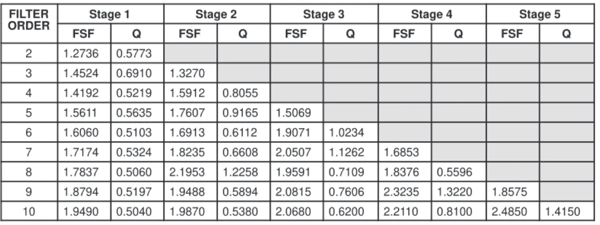
Table 2. Bessel Filter Table
FILTER
ORDER Stage 1 Stage 2 Stage 3 Stage 4 Stage 5 ORDER
FSF Q FSF Q FSF Q FSF Q FSF Q
2 1.2736 0.5773
3 1.4524 0.6910 1.3270
4 1.4192 0.5219 1.5912 0.8055
5 1.5611 0.5635 1.7607 0.9165 1.5069
6 1.6060 0.5103 1.6913 0.6112 1.9071 1.0234
7 1.7174 0.5324 1.8235 0.6608 2.0507 1.1262 1.6853
8 1.7837 0.5060 2.1953 1.2258 1.9591 0.7109 1.8376 0.5596
9 1.8794 0.5197 1.9488 0.5894 2.0815 0.7606 2.3235 1.3220 1.8575
Table 3. 1-dB Chebyshev Filter Table
FILTER
ORDER Stage 1 Stage 2 Stage 3 Stage 4 Stage 5 ORDER
FSF Q FSF Q FSF Q FSF Q FSF Q
2 1.0500 0.9565
3 0.9971 2.0176 0.4942
4 0.9932 0.7845 0.5286 3.5600
5 0.9941 1.3988 0.6552 5.5538 0.2895
6 0.9953 0.7608 0.7468 2.1977 0.3532 8.0012
7 0.9963 1.2967 0.8084 3.1554 0.4800 10.9010 0.2054
8 0.9971 0.7530 0.5538 1.9564 0.5838 2.7776 0.2651 14.2445 9 0.9976 1.1964 0.8805 2.7119 0.6623 5.5239 0.3812 18.0069 0.1593
10 0.9981 0.7495 0.7214 1.8639 0.9024 3.5609 0.4760 6.9419 0.2121 22.2779
Table 4. 3-dB Chebyshev Filter Table
FILTER
ORDER Stage 1 Stage 2 Stage 3 Stage 4 Stage 5 ORDER
FSF Q FSF Q FSF Q FSF Q FSF Q
2 0.8414 1.3049
3 0.9160 3.0678 0.2986
4 0.9503 1.0765 0.4426 5.5770
5 0.9675 2.1380 0.6140 8.8111 0.1775
6 0.9771 1.0441 0.7224 3.4597 0.2980 12.7899
7 0.9831 1.9821 0.7920 5.0193 0.4519 17.4929 0.1265
8 0.9870 1.0558 0.8388 3.0789 0.5665 6.8302 0.2228 22.8481 9 0.9897 1.9278 0.8716 4.3179 0.6503 8.8756 0.3559 28.9400 0.0983
10
Example-Circuit Test Results
To further show how to use the above information and see actual circuit performance, component values are calculated and the filter circuits are built and tested.
Figures 5 and 6 show typical component values computed for the three different filters discussed using the Sallen-Key architecture and the MFB architecture. The equivalent simplification (see Appendix A) is used for each circuit: setting the filter components as ratios and the gain equal to 1 for the Sallen-Key, and the gain equal to –1 for the MFB. The circuits and simplifications are shown for convenience. A corner frequency of 1 kHz is chosen. The values used for m and n are shown. C1 and C2 are chosen to be standard values. The values shown for R1 and R2 are the nearest standard values to those computed by using the formulas given.
– + C2
R2
C1 VO
R1 VI
Unity-Gain Sallen-Key
R1=mR, R2=R, C1=C, C2=nC, and K=1 result in: FSF×fc+ 1
2pRC mnǸ , and Q+ mn
Ǹ
m)1
FILTER TYPE n m C1 C2 R1 R2
Butterworth 3.3 0.229 0.01 µF 0.033 µF 4.22 kΩ 18.2 kΩ Bessel 1.5 0.42 0.01 µF 0.015 µF 7.15 kΩ 14.3 kΩ 3-dB Chebyshev 6.8 1.0 0.01 µF 0.068 µF 7.32 kΩ 7.32 kΩ
Figure 5. Sallen-Key Circuit and Component Values – fc = 1 kHz
R2=R, R3=mR, C1=C, C2=nC, and K=1 results in: FSF×fc+ 1
2pRC mnǸ , andQ+ mn
Ǹ
1)2m
FILTER TYPE n m C1 C2 R1 & R2 R2
Butterworth 4.7 0.222 0.01 µF 0.047 µF 15.4 kΩ 3.48 kΩ Bessel 3.3 0.195 0.01 µF 0.033 µF 15.4 kΩ 3.01 kΩ 3-dB Chebyshev 15 10.268 0.01 µF 0.15 µF 9.53 kΩ 2.55 kΩ
Figure 6. MFB Circuit and Component Values – fc = 1 kHz
The circuits are built using a TLV2772 operational amplifier, 1%-tolerance resistors, and
Figure 7 compares the frequency response of Sallen-Key and MFB second-order Butterworth filters. The frequency response of the filters is almost identical from 10 Hz to about 40 kHz. Above this, the MFB shows better performance. This will be examined latter.
f – Frequency – Hz –100
–90 –80 –70 –60 –50 –40 –30 –20 –10 0 10
GAIN vs FREQUENCY
10 100 1k 10k 100k 1M 10M
MFB Sallen-Key
Gain – dB
Figure 7. Second-Order Butterworth Filter Frequency Response
Figure 8 compares the frequency response of Sallen-Key and MFB second-order Bessel filters. The frequency response of the filters is almost identical from 10 Hz to about 50 kHz. Above this, the MFB has superior performance. This will be examined latter.
f – Frequency – Hz –100
–90 –80 –70 –60 –50 –40 –30 –20 –10 0 10
GAIN vs FREQUENCY
10 100 1k 10k 100k 1M 10M
MFB Sallen-Key
Gain – dB
Figure 9 compares the frequency response of Sallen-Key and MFB second-order 3-dB
Chebyshev filters. The frequency response of the filters is almost identical from 10 Hz to about 50 kHz. Above this, the MFB shows better performance. This will be examined shortly.
f – Frequency – Hz –100
–90 –80 –70 –60 –50 –40 –30 –20 –10 0 10
GAIN vs FREQUENCY
10 100 1k 10k 100k 1M 10M
MFB Sallen-Key
Gain – dB
Figure 9. Second-Order 3-dB Chebyshev Filter Frequency Response
Figure 10 is an expanded view of the frequency response of the three filters in the MFB topology, near fc (the Sallen-Key circuits are almost identical). It clearly shows the increased rate of attenuation near the cutoff frequency, going from the Bessel to the 3-dB Chebyshev.
–15 –10 –5 0 5
GAIN vs FREQUENCY
3-dB Chebyshev
Butterworth Bessel
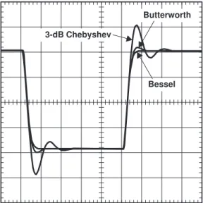
Figure 11 shows the transient response of the three filters using MFB architecture to a pulse input (the Sallen-Key circuits are almost identical). It clearly shows the increased overshoot going from the Bessel to the 3-dB Chebyshev.
3-dB Chebyshev
Butterworth
Bessel
Figure 11. Transient Response of the Three Filters
11
Nonideal Circuit Operation
Up to now we have not discussed nonideal operation of the circuits. The test results shown in Figures 7 through 9 show that at high frequency, where you expect the response to keep
attenuating at –40 dB/dec, the filters actually turn around and start passing signals at increasing amplitudes. We will now examine why this happens.
11.1 Nonideal Circuit Operation – Sallen-Key
At frequencies well above cutoff, simplified high-frequency models help show the expected behavior of the circuits. Figure 12 is used to show the expected circuit operation for a second-order low-pass Sallen-Key circuit at high frequency. The assumption made here is that C1 and C2 are effective shorts when compared to the impedance of R1 and R2 so that the amplifier’s input is at ac ground. In response, the amplifier generates an ac ground at its output, limited only by its output impedance Zo. The formula shows the transfer function of this model.
R2
VO R1
VI
Zo
VO VI+
1 R1 R2)
R1 Zo)1
VO VI[
Zo
R1Tfå )20 dBńdec Assuming Zo << R1
Zo is the closed-loop output impedance. It depends on the loop transmission and the open-loop output impedance zo: Zo+ zo
1)a(f)b , where a(f)β is the loop transmission. β is the feedback factor set by resistors R3 and R4 and is constant over frequency, but the open loop gain a(f) is dependant on frequency. With dominant-pole compensation, the open-loop gain of the amplifier decreases at –20 dB/dec over the usable frequencies of operation. Assuming that zo is mainly resistive (usually a valid assumption up to 100 MHz), Zo increases at a rate of 20 dB/dec. At high frequencies the circuit is no longer able to attenuate the input and begins to pass the signal at a 20-dB/dec rate, as the test results show.
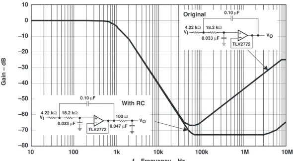
Placing a low-pass RC filter at the output of the amplifier can help nullify the feed-through of high-frequency signals. Figure 13 shows a comparison between the original Sallen-Key Butterworth filter and one using an RC filter on the output. A 100-Ω resistor is placed in series with the output, and a 0.047-µF capacitor is connected from the output to ground This places a passive pole in the transfer function at about 40 kHz that improves the high-frequency response.
f – Frequency – Hz –80
–70 –60 –50 –40 –30 –20 –10 0 10
GAIN vs FREQUENCY
10 100 1k 10k 100k 1M 10M
– + 0.10 µF
0.033 µF VO 4.22 kΩ
VI 18.2 kΩ 100 Ω
0.047 µF TLV2772
– + 0.10 µF
0.033 µF VO 4.22 kΩ
VI
18.2 kΩ
TLV2772
With RC
Original
Gain – dB
11.2 Nonideal Circuit Operation – MFB
The high-frequency analysis of the MFB is very similar to the Sallen-Key. Figure 14 is used to show the expected circuit operation for a second-order low-pass MFB circuit at high frequency. The assumption made here is that C1 and C2 are effective shorts when compared to the impedance of R1, R2, and R3. Again, the amplifier’s input is at ac ground, and generates an ac ground at its output limited only by its output impedance Zo. Capacitor Cp represents the parasitic capacitance from VI to VO. The ability of the circuit to attenuate high-frequency signals is dependent on Cp and Zo. The impedance of Cp decreases at –20 dB/dec and Zo increases at 20 dB/dec. The overall transfer function turns around at high frequency to
40 dB/dec as seen in the laboratory data. Spice simulation shows that as little as 0.4 pF will produce the high-frequency feed through observed.
VO Cp
VI
Zo
VO VI[
Zo 1 2pfCp)Zo
Tf2å )40 dBńdec
Figure 14. Second-Order Low-Pass MFB High-Frequency Model
Care should be taken when routing the input and output signals to keep capacitive coupling to a minimum.
Placing a low-pass RC filter at the output of the amplifier can help nullify the feed through of high-frequency signals. Figure 15 below shows a comparison between the original MFB Butterworth filter with one using an RC filter on the output. A 100-Ω resistor is placed in series with the output, and a 0.047-µF capacitor is connected from the output to ground. This places a passive pole in the transfer function at about 40 kHz that improves the high-frequency response.
f – Frequency – Hz –110 –100 –90 –80 –70 –60 –50 –40 –30 –20 –10 0 10 GAIN vs FREQUENCY
10 100 1k 10k 100k 1M 10M
VO VI
15.5 kΩ 3.48 kΩ
0.01 µF 15.5 kΩ
0.047 µF
100 Ω
0.047 µF
TLV2772
VO VI
15.5 kΩ
+ – 3.48 kΩ
0.01 µF 15.5 kΩ
0.047 µF
TLV2772
+ –
Original
With RC
Gain – dB
12
Comments About Component Selection
Theoretically, any values of R and C which satisfy the equations might be used, but practical considerations call for certain guidelines to be followed.
Given a specific corner frequency, the values of R and C are inversely proportional to each other. By making C larger R becomes smaller, and vice versa.
Making R large may make C so small that parasitic capacitors cause errors. This makes smaller resistor values preferred over larger resistor values.
The best choice of component values depends on the particulars of your circuit and the tradeoffs your are willing to make. Adhering to the following general recommendations will help reduce errors:
•
Capacitors– Avoid values less than 10 pF – Use NPO or COG dielectrics – Use 1%-tolerance components – Surface mount is preferred.
•
Resistors– Values in the range of a few-hundred ohms to a few-thousand ohms are best. – Use metal film with low-temperature coefficients.
– Use 1% tolerance (or better). – Surface mount is preferred.
13
Conclusion
We have investigated building second-order low-pass Butterworth, Bessel, and 3-dB Chebyshev filters using the Sallen-Key and MFB architectures. The same techniques are extended to higher-order filters by cascading second-order stages for even order, and adding a first-order stage for odd order.
The advantages of each filter type come at the expense of other characteristics. The Butterworth is considered by a lot of people to offer the best all-around filter response. It has maximum flatness in the pass-band with moderate rolloff past cutoff, and shows only slight overshoot in response to a pulse input.
The Bessel is important when signal-conditioning square-wave signals. The constant-group delay means that the square-wave signal is passed with minimum distortion (overshoot). This comes at the expense of a slower rate of attenuation above cutoff.
Tables 5 and 6 give a brief summary of the previous trade-offs.
Table 5. Summary of Filter Type Trade-Offs
FILTER TYPE ADVANTAGE(s) DISADVANTAGE(s)
Butterworth Maximum pass-band flatness Slight overshoot in response to pulse input and moderate rate of attenuation above fc
Bessel Constant group delay – no overshoot with pulse input Slow rate of attenuation above fc
3-dB Chebyshev Fast rate of attenuation above fc Large overshoot and ringing in response to pulse input
Table 6. Summary of Architecture Trade-Offs
ARCHITECTURE ADVANTAGE(s) DISADVANTAGE(s)
Sallen-Key Not sensitive to component variation at unity gain High-frequency response limited by the frequency response of the amplifier
MFB Less sensitive to component variations and superior high-frequency response
Appendix A
Filter-Design Specifications
A.1
Sallen-Key Design Simplifications
Depending upon how you go about working the equations which describe the Sallen-Key
transfer function, filter design can be simple or tedious. The following simplifications can be used to ease design, but note that the easier the design becomes, the more it limits the design
freedom.
A.1.1
S-K Simplification 1: Set Filter Components as Ratios
Letting R1=mR, R2=R, C1=C, and C2=nC, results in: FSF fc+ 1
2pRC mnǸ and
Q+ Ǹmn
m)1)mn(1–K). This is the most rudimentary of simplifications. Design should start by determining the ratios m and n required for the gain and Q of the filter, and then selecting C and calculating R to set fc.
A.1.2
S-K Simplification 2: Set Filter Components as Ratios and Gain = 1
Letting R1=mR, R2=R, C1=C, C2=nC, and K=1 results in: FSF fc+ 1
2pRC mnǸ and Q+ Ǹmn
m)1. This sets the gain = 0 dB in the pass band. Design should start by determining the ratios m and n for the required Q of the filter, and then selecting C and calculating R to set fc.
A.1.3
S-K Simplification 3: Set Resistors as Ratios and Capacitors Equal
Letting R1=mR, R2=R, and C1=C2=C, results in: FSF fc+ 1
2pRC mǸ and Q+
m
Ǹ
1)m (2–K). The main motivation behind setting the capacitors equal is the limited selection of values in comparison to resistors.
There is interaction between setting fc and Q. Design should start with choosing m and K to set the gain and Q of the circuit, and then choosing C and calculating R to set fc.
A.1.4
S-K Simplification 4: Set Filter Components Equal
Letting R1=R2=R and C1=C2=C results in: FSF fc+ 1
2pRC and Q+ 1
A.2.1
MFB Simplification 1: Set Filter Components as Ratios
Letting R2=R, R3=mR, C1=C, and C2=nC, results in: FSF fc+ 1
2pRC mnǸ and
Q+ Ǹmn
1)m (1–K). This is the most rudimentary of simplifications. Design should start by determining the ratios m and n required for the gain and Q of the filter, and then selecting C and calculating R to set fc.
A.2.2
MFB Simplification 2: Set Filter Components as Ratios and Gain = –1
Letting R2=R, R3=mR, C1=C, C2=nC and K= –1 results in: FSF fc+ 1
2pRC mnǸ and Q+ Ǹmn
Appendix B
Higher-Order Filters
B.1
Higher Order Filters
It was stated earlier that higher order filters can be constructed by cascading second-order stages for even-order, and adding a first-order stage for odd-order. To show how this is accomplished we will consider two examples: constructing a fifth-order Butterworth filter, and then a sixth-order Bessel filer.
By breaking higher than second-order filters into complex-conjugate-zero pairs, second-order stages are constructed that, when cascaded, realize the overall polynomial. For example, a sixth-order filter will have three complex-zero pairs and can be written as:
P6th(s) = (s2+ z1)(s + z1*)(s + z2)(s +z2*)(s +z3)(s +z3*). Each of the complex-conjugate-zero pairs can be multiplied out and written as:
(s + z1)(s + z1*) = s2 + a11s + a01 (s + z2)(s + z2*) = s2 + a12s + a02 (s + z3)(s + z3*) = s2 + a13s + a03
The overall polynomial is then reconstructed in the following form: P6th(s) = (s2 + a11s + a01)(s2 + a12s + a02)(s2 + a13s + a03)
B.1.1
Fifth-Order Low-Pass Butterworth Filter
Referring to Table 1, for a fifth-order Butterworth filter we can write the required circuit transfer function as:
HLP(f)+ K
ǒ
jffc)1
Ǔ
ǒ
–ǒ
fcfǓ
2
)0.61801 fcjf )1
Ǔǒ
–ǒ
f fcǓ
2
)0.61801 fcjf )1
Ǔ
Figure B–1 shows a Sallen-Key circuit implementation and the required component values. fc is the –3-dB point. The overall gain of the circuit in the pass band is K = Ka × Kb.
– + C2a
R2a
C1a
R4a R3a R1a
– + C2b
R2b
C1b
R4b R3b
VO R1b
– + R
VI
Stage 1 (See Table)
Stage 2 (See Table)
Stage 3 (See Table)
C
STAGE fc Q K
1 1
2pRC NA 1
2 1
2pǸR1aR2aC1aC2a
R1aR2aC1aC2a
Ǹ
R1aC1a)R2aC1a)R1aC2a(1–Ka)+0.618 Ka+
R3a)R4a R3a
3 1
2pǸR1bR2bC1bC2b
R1bR2bC1bC2b
Ǹ
R1bC1b)R2bC1b)R1bC2b(1–Kb)+1.618 Kb+
R3b)R4b R3b
B.1.2
Sixth-Order Low-Pass Bessel Filter
Referring to Table 2 for a sixth-order Bessel filter, we can write the required circuit transfer function as:
HLP(f)+ K
ǒ
–ǒ
f 1.6060fcǓ
2
)1.2202 jf
fc)1
Ǔǒ
–ǒ
f 1.6913fcǓ
2
)0.9674 jf
fc)1
Ǔǒ
–ǒ
f 1.9071fcǓ
2
)0.5124 jf fc)1
Ǔ
Figure B–2 shows a MFB circuit implementation and the required component values. fc is the –3-dB point. The overall gain of the circuit in the pass band is K = Ka × Kb × Kc.
+ – C1a C2a R1a Vin R3a R2a + – C1b C2b R1b R3b R2b + – C1c C2c R1c R3c R2c Vout Stage 2 (See Table) Stage 1 (See Table) Stage 3 (See Table)
STAGE fc Q K
1 1
1.6060 2pǸR2aR3aC1aC2a
R2aR3aC1aC2a
Ǹ
R3aC1a)R2aC1a)R3aC1a(–Ka)+0.5103 Ka+ –R2a
R1a
2 1
1.6913 2pǸR2bR3bC1bC2b
R2bR3bC1bC2b
Ǹ
R3bC1b)R2bC1b)R3bC1b(–Kb)+0.6112 Ka+ –R2b
R1b
3 1
1.9071 2pǸR2cR3cC1cC2c
R2cR3cC1cC2c
Ǹ
R3cC1c)R2cC1c)R3cC1c(–Kc)+1.0234 Kb+ –R2c
R1c
Texas Instruments and its subsidiaries (TI) reserve the right to make changes to their products or to discontinue any product or service without notice, and advise customers to obtain the latest version of relevant information to verify, before placing orders, that information being relied on is current and complete. All products are sold subject to the terms and conditions of sale supplied at the time of order acknowledgment, including those pertaining to warranty, patent infringement, and limitation of liability.
TI warrants performance of its semiconductor products to the specifications applicable at the time of sale in accordance with TI’s standard warranty. Testing and other quality control techniques are utilized to the extent TI deems necessary to support this warranty. Specific testing of all parameters of each device is not necessarily performed, except those mandated by government requirements.
Customers are responsible for their applications using TI components.
In order to minimize risks associated with the customer’s applications, adequate design and operating safeguards must be provided by the customer to minimize inherent or procedural hazards.
TI assumes no liability for applications assistance or customer product design. TI does not warrant or represent that any license, either express or implied, is granted under any patent right, copyright, mask work right, or other intellectual property right of TI covering or relating to any combination, machine, or process in which such semiconductor products or services might be or are used. TI’s publication of information regarding any third party’s products or services does not constitute TI’s approval, warranty or endorsement thereof.