Maria Inês Gonçalves Monteiro
Licenciatura em Ciências da Engenharia Química e Bioquímica
Forward osmosis membranes tailored by hydrogel
coatings
Dissertação para obtenção do Grau de Mestre
em Engenharia Química e Bioquímica
Orientador:
Professor Andrew Livingston e Professora Isabel Coelhoso
Co-orientador:
Ruslan Kochanov
Júri:
Presidente: Professora Doutora Maria Ascensão C. F. Miranda Reis Arguente: Doutor Svetlozar Gueorguiev Velizarov
Maria Inês Gonçalves Monteiro
Forward osmosis membranes tailored by hydrogel
coatings
Dissertação para obtenção do Grau de Mestre
em Engenharia Química e Bioquímica
Copyright Maria Inês Gonçalves Monteiro, FCT-UNL, UNL
Acknowledgements
I would like to express my deep gratitude to Professor Andrew
Livingston (Imperial College, London) and Professor Isabel
Coelhoso (Faculdade de Ciências e Tecnologia, Universidade
Nova de Lisboa), for all their useful and constructive
recommendations on this project. I also would like to thank,
Ruslan Kochanov (Imperial College, London), for his guidance,
patience and useful elucidations.
I would also like to thank Andrew’s group for their support and
III
ABSTRACT
Forward osmosis (FO) is a promising process to substitute reverse osmosis (RO), as a lower
cost and more environmentally friendly desalination process. However, FO still presents some
drawbacks, in particular the several internal concentration polarization (CP) effects and
insufficient salt selectivity. In order to overcome these disadvantages, this study focuses on the
use of hydrogel surface-coated FO membranes to minimize internal CP effect in water
purification, and also to improve membrane salt rejection. For this, a series of crosslinked
poly(ethylene glycol) (PEG)-based hydrogels were synthesized, by the photopolymerization of
poly(ethylene glycol) diacrylate (PEGDA) and the monomer (PEG) in the presence of a
photoinitiator. The water uptake and salt permeability of the resulting films were controlled by
manipulating the composition ratio of PEGDA and the monomer PEG, by varying the water
content in the prepolymerization mixture and the UV-exposure time. High water uptake and low
salt permeability values were observed for the films prepared with 50wt% of water content
(50%PEGDA). The hydrogels were applied using different techniques (pressure, soaking and
coating) to a cellulose acetate (CA) membrane prepared by phase inversion. However, only one
technique was effective, surface coating. The CA membranes coated with these hydrogels
materials showed an improvement in NaCl rejection (≅100%) and in some cases an
enhancement of 100 and 120% of the original water flux (50% PEGDA coating on the active
layer and on the porous support, respectively; in PRO mode). The 50%PEGDA coated
membrane (with a coating on the porous support) has also shown reduction of the internal CP
effects.
IV
RESUMO
A osmose direta (OD) é um processo promissor para substituição da osmose inversa no
processo de dessalinização, já que é mais económico e menos prejudicial para o meio
ambiente. No entanto, a OD ainda apresenta alguns inconvenientes, nomeadamente o efeito
de polarização da concentração (PC) interna e baixa seletividade. De forma a contornar estes
problemas, o presente estudo tem como objetivo a preparação de membranas de OD
revestidas por um hidrogel, a fim de minimizar o efeito de PC interna e também melhorar a
rejeição da membrana aos sais. Para tal, diferentes hidrogéis de polietileno glicol (PEG) foram
preparados através da fotopolimerização de diacrilado de polietileno glicol (PEGDA) e do
monómero PEG, na presença de um fotoiniciador. A absorção de água e a permeabilidade ao
sal dos filmes preparados foram controlados pela variação das razões de PEGDA e do
monómero PEG, pela variação do teor de água na mistura de prepolimerização e pela variação
do tempo de exposição à luz UV. Os filmes preparados com 50% de teor em água
(50%PEGDA) obtiveram elevados valores de absorção de água e baixos valores de
permeabilidade ao sal. Os hidrogéis foram aplicados através de diferentes técnicas (pressão,
imersão e revestimento) a uma membrana de acetato de celulose (AC), preparada pela técnica
de inversão de fase. Porém, apenas uma das técnicas resultou, o revestimento de superfície.
Assim, as membranas AC revestidas com hidrogel apresentaram uma rejeição ao NaCl
superior (≅100%) e, em alguns casos, uma melhoria de 100 e 120% do fluxo de água original
(para as membranas com revestimento de 50%PEGDA na camada activa e suporte poroso,
respectivamente; no modo PRO). Igualmente, a membrana revestida com 50%PEGDA
(revestimento sobre o suporte poroso) apresentou uma redução do efeito de PC interna.
V
INDEX
1. INTRODUCTION ... 1
2. FORWARD OSMOSIS PROCESS ... 2
2.1. Overall advantages of Forward Osmosis ... 5
2.2. System thermodynamics ... 6
2.3. Concentration polarization and fouling in osmotic processes ... 13
a. External concentration polarization ... 14
b. Internal concentration polarization ... 16
c. Membrane fouling ... 20
2.4. Reverse solute diffusion ... 21
2.5. Draw solutions ... 22
a. Permeate recovery ... 25
2.6. Membrane types ... 26
2.7. Membranes modules and devices ... 32
a. Plate-and-frame ... 33
b. Spiral wound ... 34
c. Tubular ... 35
d. Hydration bags ... 36
2.8. Applications of forward osmosis ... 36
a. Waste water treatment ... 37
b. Hydration bags ... 43
c. Seawater desalination ... 44
d. Power generation ... 45
e. Food processing ... 47
VI
g. Other applications ... 49
3. MOTIVATION AND OBJECTIVES ... 52
4. MATERIALS AND METHODS ... 56
4.1. Materials ... 56
4.2. Membrane preparation ... 56
4.3. Hydrogel synthesis and characterization ... 57
4.4. Hydrogel films characterization ... 59
a. Water transport properties ... 59
b. Salt transport properties ... 60
4.5. Membrane characterization ... 61
a. Membrane porosity, ... 61
b. Thickness, ... 62
c. Water uptake ... 62
d. Scanning electron microscopy (SEM) ... 62
e. Digital microscope ... 62
f. Thermogravimetric analysis (TGA) ... 62
g. Water contact angle ... 63
4.6. Membrane performance in FO ... 63
4.7. The influence of hydrogel thickness in water flux ... 65
4.8. Determination of external mass transfer coefficients in the FO cell ... 65
5. RESULTS AND DISCUSSION ... 68
5.1. Determination of external mass transfer coefficients in the FO cell ... 68
5.2. The effect of solvent/co-solvent ratio on membrane performance ... 69
a. Membranes morphology ... 69
VII
c. Membrane parameters ... 71
5.3. Cellulose acetate membrane performance ... 72
5.4. The effect of the porous support on the membrane performance ... 73
a. Membrane performance ... 74
b. Membrane parameters ... 75
5.5. PEG-based hydrogel free-standing films characterization ... 75
5.6. The influence of PEG-based hydrogel coatings on membrane performance . 79 a. Membrane morphology observations ... 79
b. The influence of the hydrogel thickness in water flux ... 83
c. Thermogravimetric analisys ... 84
d. Coated membranes performance ... 85
e. Coated membranes water transport properties ... 94
f. Coated membranes parameters ... 95
6. CONCLUSIONS ... 98
7. FUTURE WORK ... 98
8. BIBLIOGRAPHY ... 100
Appendixes ... 116
Appendix 1 - Techniques for membrane preparation ... 116
a. Phase inversion method ... 117
b. Factors affecting membrane structure ... 120
Appendix 2 - Membrane surface modification ... 122
a. Physical method ... 123
IX
FIGURES CAPTION
Figure 1 – Schematic illustration of osmosis and osmotic pressure (Rogers, et al., 2000) ... 2
Figure 2- Solvent flows in FO and RO. For FO, ∆P is approximately zero and water diffuses
to the more saline side of the membrane. For RO, water diffuses to the less saline side due to
hydraulic pressure (∆P>∆π) (Cath, et al., 2006). ... 4
Figure 3- Molecular transport through membranes can be described by a flow through
permanent pores (a) or by the solution-diffusion mechanism (b) (Baker, 2000) ... 7
Figure 4- Pressure driven permeation of one-component solution through a membrane
according to the solution-diffusion transport model, where = (Baker, 2000) ... 8
Figure 5 - Chemical potential, pressure, and solvent activity profiles through an osmotic
membrane following the solution-diffusion model. The pressure in the membrane is uniform and
equal to the high-pressure value, so the chemical potential gradient within the membrane is
expressed as concentration gradient (where = ) (Baker, 2000) ... 9
Figure 6- Flux decrease as function of time due to the combined effect of fouling and
concentration polarization (Crespo, et al., 2005) ... 14
Figure 7 – Illustrations of driving forces profiles, expressed as water chemical potential, ,
for osmosis several membrane types and orientations. (a) A symmetric dense membrane. (b)
An asymmetric membrane with the porous support layer against the feed solution; the profile
illustrates concentrative internal CP. (c) An asymmetric membrane with the dense layer against
the feed solution; the profile illustrates dilutive internal CP. The actual (effective) driving force is
represented by ∆ . External CP effects on the driving force are assumed to be negligible in
this figure (McCutvheon, et al., 2006). ... 17
Figure 8- Illustration of osmotic driving force profiles for osmosis through several membrane
types and orientations, incorporating both internal CP and external CP. (a) Symmetric dense
membrane; the profile illustrates concentrative and dilutive external CP. (b) An asymmetric
membrane with the dense active layer against the draw solution (PRO mode); (c) An
asymmetric membrane with the porous support layer against the draw solution (FO mode); the
profile illustrates dilutive internal CP and concentrative internal CP. Key: , is the bulk draw
X the bulk feed osmotic pressure, , is the membrane surface osmotic pressure on the feed
side, , is the effective osmotic pressure of the feed in PRO mode, , is the effective
osmotic pressure of the draw solution in FO mode, ∆ is the osmotic pressure difference
across the membrane, and ∆ is the effective osmotic driving force (McCutcheon, et al.,
2006) ... 18
Figure 9 – A conceptual illustration of the effect of draw solute reverse diffusion on
cake-enhanced osmotic pressure (CEOP) in FO for different draw solutions: a) NaCl and B) dextrose
(Lee, et al., 2010) ... 21
Figure 10- Daily requirement of draw solute replenishment (kg/d) as function of water
production (m3/d) derived based on equation (25) for the three scenarios: (A) =0.01 g.L-1;
(B) =0.1 g.L-1; and (C) =1 g.L-1 (Qin, et al., 2012) ... 23
Figure 11 - Osmotic pressures as a function of solution concentration at 25º C for various
potential draw solutions. Data were calculated using OLI Stream Analyzer 2.0 (Cath, et al.,
2006) ... 25
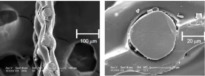
Figure 12 – SEM photographs of cross sections of forward osmosis (CTA) membrane of
HTI’s FO membrane. A polyester mesh is embedded between the polymer material for
mechanical support. The membrane thickness is less than 50 µm, much thinner than the RO
membranes used (McCutcheon, et al., 2005). ... 28
Figure 13 – Flows in FO and PRO processes. Feed water flows on the active side of the
membrane and draw solution flows counter-currently on the support side of the membrane. In
PRO, the draw solution is pressurized and is released in a turbine to produce electricity (Cath,
et al., 2006) ... 32
Figure 14 – Cross-section of plate-and-frame module, (⊙) Flow of the draw in one direction;
(⊗) Flow of draw in the other direction; gray area – flow of the feed; Cross-hatched area –
polycarbonate areas (Cath, et al., 2005) ... 34
Figure 15- Schematic representation of a RO spiral-wound module ... 34
Figure 16- Flow patterns in a spiral-wound module modified for FO. The feed solution flows
through the central tube into the inner side of the membrane envelope and the draw solution
flows in the space between the rolled envelopes (Cath, et al., 2006; Mehta, 1982). ... 35
XI Figure 18 - water flux as a function of draw solution (DS) concentration during FO
concentration of (a) pretreated centrate and (b) non-treated centrate. Flux decline between trials
is due to organic and suspended solids fouling (Holloway, et al., 2007) ... 42
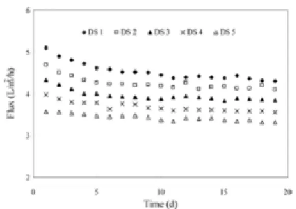
Figure 19 - Variation in water flux with the operation time under different DS concentrations ... 43
Figure 20 – Illustration of water purification hydration bag (Cath, et al., 2006) ... 44
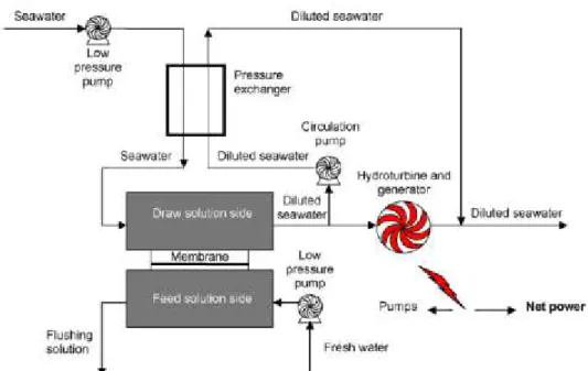
Figure 21- Schematic of a pressure-retarded osmosis (PRO) power plant (Achilli, et al., 2009) ... 46
Figure 22- Schematic representation of FO applications for osmotic drug delivery systems. A) Schematic view of the asymmetric membrane capsule (Thombre, et al., 1999); B) Principle of the three-chamber Rose-Nelson osmotic pump first described (Santus, et al., 1995) ... 49
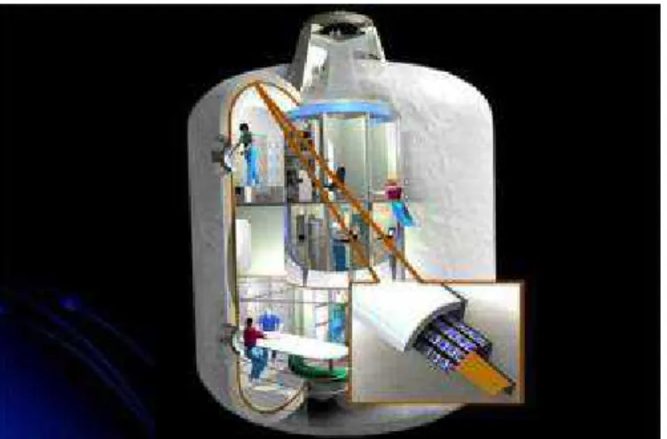
Figure 23- Schematic of the Offshore Membrane Enclosure for Growing Algae (OMEGA) system. Inset shows the permeation through and rejection by FO membrane in contact with the seawater. The top of the enclosure, which is in contact with atmosphere, contains specialized membranes that allow the passage of sunlight and the exchange of CO2/O2 to facilitate the algae photosynthesis (Hoover, et al., 2011) ... 50
Figure 24- Chemical structure of hydrogel components; PEG- poly(ethylene glycol) monomer, PEGDA-poly(ethylene glycol) diacrylate ... 53
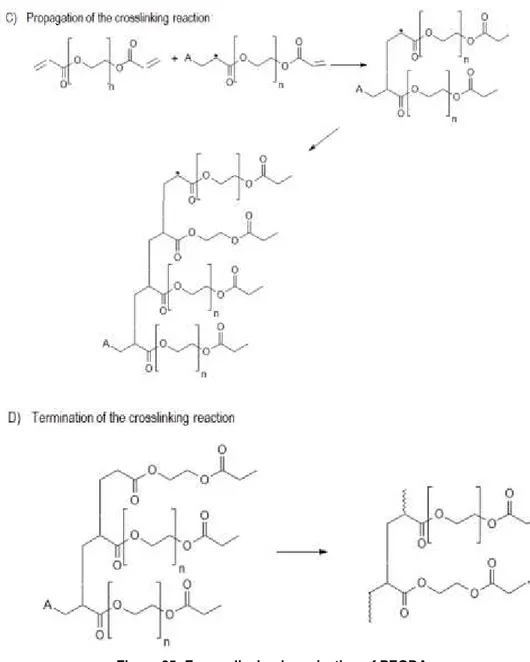
Figure 25- Free radical polymerization of PEGDA ... 54
Figure 26- Illustration of the expected hydrogel treatment effect on the membranes ... 54
Figure 27 - Schematic illustration of membrane treatments used ... 59
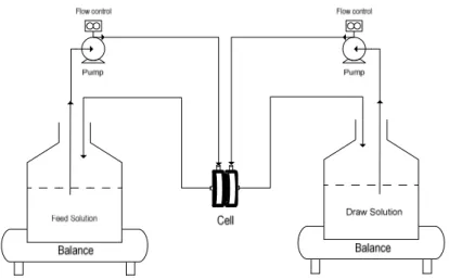
Figure 28- Schematic diagram of the lab-scale FO experimental set-up... 63
Figure 29- SEM image of membrane cross-section: A) Membrane A; B) Membrane B; C) Membrane C and D) Membrane D ... 69
Figure 30- Base membrane water flux over a range of osmotic pressure differences; PRO mode. The theoretical line was illustrated by considering Aw constant ... 73
Figure 31 – Performance of the CA membranes prepared with different porous supports, test in PRO mode ... 74
XII Figure 33 – Digital microscope images of top surface morphology, at 200x, of the A)
untreated membrane; B) membrane with one PEDGA (prepolymerization mixture of 50wt%
PEGDA ) top coating; C) membrane soaked for 2 hours on a PEGDA solution; D) membrane
with one top coat (prepolymerization mixture of PEG35000/PEGDA) ... 79
Figure 34 - Digital microscope images of bottom surface morphology, at 200x, of the A)
untreated membrane; B) membrane with one PEDGA (prepolymerization mixture of 50wt%
PEGDA ) bottom coating; C) membrane soaked for 2 hours on a PEGDA solution; D)
membrane with one bottom coat (prepolymerization mixture of PEG35000/PEGDA) ... 80
Figure 35- Top surface image of: A) untreated membrane, B) Membrane with a top coat of
50% PEGDA, C) Membrane with a top coat of PEG3000/PEGDA, D) Membrane with a top coat
of PEG35000/PEGDA ... 81
Figure 36 - Cross-section image of: A) untreated membrane, B) Membrane with a top coat of
50% PEGDA, C) Membrane with 3 top coatings of 50% PEGDA D) Membrane with a top coat of
PEG3000/PEGDA, E) Membrane with a top coat of PEG35000/PEGDA... 82
Figure 37 – Bottom surface image of: A) untreated membrane, B) Membrane with a bottom
coat of 50% PEGDA, C) Membrane with a bottom coat of PEG35000/PEGDA ... 83
Figure 38 - The influence of hydrogel thickness in water flux ... 84
Figure 39- TGA curves of the individual membrane components ... 84
Figure 40 – TGA curves of the untreated membrane and the membranes prepared with
different hydrogels impregnations techniques (coating and soaking) ... 85
Figure 41- Effect of the hydrogel top coating on the membrane flux; left side PRO mode and
right side FO mode ... 87
Figure 42 - Effect of the hydrogel bottom coating on the membrane flux; left side PRO mode
and right side FO mode ... 89
Figure 43- Effect of the 3 coatings of hydrogel on the membrane flux; left side PRO mode
and right side FO mode ... 91
Figure 44 – 50% Coated and base membrane performance over a range of osmotic pressure
differences; PRO mode ... 92
Figure 45 – Draw solution salt concentration over time; performance of 50% coated
XIII Figure 46- Scanning electron micrographs of membrane cross sections with typical
structures: a) Asymmetric membrane with uniform-pore substructure; b) Asymmetric membrane
with a graded-pore substructure; c) Asymmetric membrane with a finger-pore substructure; d)
Symmetric microporous membrane without a skin (Kock, et al., 1977). ... 117
Figure 47-Schematic phase diagram of the system polymer-solvent-precipitant showing the
precipitation pathway of the casting solution during membrane formation (Kock, et al., 1977).
... 119
Figure 48 – Schematic diagrams of antifouling mechanisms: (a) pure water layer; (b)
XIV
TABLES CAPTION
Table 1 - Summary of the main properties of the osmotically-driven separation processes
(Khayet, et al., 2011; Achilli, et al., 2009; Qin, et al., 2012; Gostoli, 1999) ... 4
Table 2- The Comparisons between RO and FO (Liu, et al., 2009) ... 5
Table 3 – Additional operating costs to a FO desalination plant for replenishment of lost draw solutes(Qin, et al., 2012) ... 24
Table 4 – FO performance of CTA-FO membrane from HTI ... 28
Table 5- Recent FO membranes developed ... 30
Table 6- Nomenclature of membranes used to test the effect of solvent/co-solvent ratio on membrane performance ... 57
Table 7 – Composition of the hydrogels prepared ... 58
Table 8- Mass-transfer coefficients of the FO test solutes obtain form the benzoic acid dissolution experiments ... 68
Table 9 - Performance of the CA membranes in the FO system ... 70
Table 10- Parameters of the CA membranes ... 72
Table 11- Characteristics of the base CA membrane, with different porous support ... 74
Table 12- Parameters of the base CA membrane, with different porous supports. ... 75
Table 13 – Water transport properties of free-standing hydrogel films ... 76
Table 14 - Salt transport properties of free-standing hydrogel films ... 77
Table 15- Performance of CA membrane, untreated and prepared with 1 coating on the top of the active layer. ... 86
Table 16 - Performance of CA membrane, untreated and prepared with 1 coating on the top of the porous support layer. ... 88
Table 17- Performance of CA membrane, untreated and prepared with 3 coating on the top/bottom ... 90
Table 18- Performance of CA membrane, untreated and prepared by soaking ... 91
Table 19- Water flux and NaCl rejection results for the FO runs carried out under settled feed solution concentration and increasing draw solution concentration (PRO mode) ... 92
XV Table 21 – Membrane water uptakes... 94
Table 22 - Membrane parameters. ... 95
XVII
ABREVIATIONS
AA - Acrylic acid
AMPS - 2-acrylamido-2-methylpropane-sulfonic acid
CA - Cellulose Acetate
CEOP - Cake-enhanced osmotic pressure
CP - Concentration polarization
CTA - Cellulose triacetate DIW - Deionized water
FO - Forward Osmosis
HTI - Hydration Technologies Inc
ICP - Internal concentration polarization
iCVD - Initiated chemical vapour deposition
MA - Methacrylic acid
MD - Membrane distillation
Mw - Molecular weight
NF - Nanofiltration
OMBR - Osmotic membrane bioreactor
OMD - Osmotic membrane distillation
PEGDA - Poly(ethylene glycol) diacrylate
PEGDE - Poly(ethylene glycol) diglycidyl ether
PEGMA - Poly(ethylene glycol) methacrylate
PRO - Pressure retarded osmosis
RO - Reverse osmosis
SPM - 3- sulfopropylmethacrylate
TGA - Thermogravimetric analysis
TFC - Thin film composite
UF - Ultrafiltration
XIX
NOMENCLATURE
∗ - Solubility of benzoic acid in water (mol.m-3
)
- Concentration of benzoic acid in water (mol.m-3)
- Hydraulic diameter (m)
- Mass transfer cefficient (m.s-1)
- Thickness (µm)
!" - Mass of the dry hydrogel film (g) #$% - Mass of the wet hydrogel film (g)
& - Time (h)
' - Membrane water permeability (L.m-2.h-1.bar-1)
'( - Membrane surface area (m2)
) - Membrane salt permeability (L.m-2.h-1.bar-1)
*+ - Salt diffusivity coefficient (m2.s-1)
,- - Flux of component i (L.m-2.h-1)
,. - Water flux (L.m-2.h-1)
,/ - Salt flux (g.m-2.h-1)
0+ - Salt permeability coefficient (m2.s-1)
1+ - Salt partition coefficient
R - Ideal gas constant (J. K-1.mol-1)
2 - Solute rejection (%)
T - Temperature (K)
Re - Reynolds number
+ - Structural parameter (mm)
Sc - Schmidt number
XXI
GREEK SYMBOLS
3# - Water uptake (%)
4* - Osmotic pressure of the draw solution (bar)
45 - Osmotic pressure of the feed solution (bar)
∆4 - Osmotic pressure difference (bar)
∆4677 - Effective osmotic pressure difference driving force (bar)
∆4( - Osmotic pressure difference across the membrane (bar)
8 - Osmotic coefficient (bar.dm3.g-1)
∆0 - Pressure difference (bar)
∆9:;< - Water volume variation in the draw/feed solution (dm
3
)
=. - Mass density of water (g.dm-3)
=> - Mass density of polymer (g.dm-3) - Porosity (%)
? - Tortuosity
@ - Chemical potential (energy/mole)
1
1. INTRODUCTION
Water scarcity and the lack of drinking water are the most serious challenges of the
twenty-first century. Currently, one third of the world’s population lives in water-stressed countries and,
by 2025, this figure is expected to rise to two-thirds (Elimelech, 2006). Increasing population
growth and a warming global climate have created even greater disparities between the
supplies of, and demands for, reliable fresh water sources. In several cases, conflicts over
shared water have exacerbated already significant tensions between neighbouring states
(McGinnis, et al., 2010). The need to alleviate water scarcity and ensure good water quality is a
major challenge.
In highly industrialized countries, there are growing problems of providing adequate water
supply and properly disposal of municipal and industrial used water. In developing countries,
particularly those in arid parts of the world, there is a need to develop low-cost methods of
acquiring new water supply while protecting existing water sources from pollution.
Under the threats of fresh water shortage, many engineers and researchers have been
dealing with reclaiming polluted water, while others try to find other alternative sources. To
overcome this problem, the desalination of seawater and other water sources, is becoming a
more and more attractive method to produce high quality water for both industrial and domestic
usage. Seawater and brackish water desalination technologies hold great promise to reduce
water scarcity in arid and densely populated regions of the world. In pursuit of these goals,
some techniques have already been developed, as multi-effect distillation, multistage flash,
vapor compression, and the most popular reverse osmosis (RO) (Karagiannis, et al., 2008).
The reverse osmosis (RO) is a membrane separation process, which its main application is
water treatment (seawater desalination, wastewater treatment, brackish water and water
purification) (Cath, et al., 2006; Kim, et al., 2008; Peñate, et al., 2012). In this process, the water
is forced to move across a selective permeable membrane against a concentration gradient, by
applying pressure (greater than the osmotic pressure) (Cath, et al., 2006). Nevertheless, the RO
process has some unavoidable disadvantages the energy costs of seawater and brackish water
by RO desalination is too high for economic widespread use; it has also large brine discharge
2 cost (McGinnis, et al., 2010; Lee, et al., 2010). So, is important to find an alternative method for
water purification and desalination, which lead to a process less expensive and easy to operate.
In order to address some of the challenges still facing current seawater and brackish water
desalination technologies, forward osmosis (FO) has gained attention as a possible solution.
2. FORWARD OSMOSIS PROCESS
Lately there has been an increase interest, of using the osmosis phenomenon or forward
osmosis (FO) for water treatment instead of the RO process. The osmosis phenomenon was
discovered by Nollet in 1748 (Nollet, et al., 1748), although few studies were conducted before
the progress of membrane technology. Only in the past years the interests in osmotically driven
processes has increased.
In osmotically driven membrane processes two solutions with different salt concentration are
separated by a semipermeable membrane, which only allows small molecules (like
water-molecules) pass. The difference of concentration between the two solutions creates a gradient
that drives water across the membrane from the side of low salt concentration to the side of
high salt concentration. An osmotic pressure ( ) arises due to this concentration difference (see
Figure 1), which is the pressure that applied to the more concentrated solution would prevent
transport of water across the membrane.
3 The solute concentration (BC) and the osmotic pressure ( ) can be related by the van’t Hoff
equation, which is:
=DEFG
HI (1)
Where J is the universal gas constant, K is the temperature and LM is the molecular weight.
It can be seen, in equation (1), that the osmotic pressure is proportional to the concentration
and inversely proportional to the molecular weight (LM). If the solute dissociates (as for instance
salts) or associates, equation (1) must be modified. When dissociation occurs the number of
moles increases and hence the osmotic pressure increases proportionally, whereas in the case
of association the number of moles decreases as does the osmotic pressure. Substantial
deviations from the van’t Hoff law occur at high concentrations and with macromolecular
solutions (Mulder, 1996).
For salt solutions the following van’t Hoff equation is used:
= . O. BC. J. K (2)
Where, is the number of ions and O is the osmotic coefficient.
Osmotically-driven membrane processes can be classified as forward osmosis (FO),
pressure retarded osmosis (PRO, see section 2.8 d) and osmotic membrane distillation (OMD).
This latter process, unlike FO and PRO, uses a porous hydrophobic membrane to separate two
solutions (feed and osmotic solution) with different solute concentrations. The water passes
through the membrane in the form of vapour, from the surface of the solution with higher vapor
pressure (feed) to the surface of the solution with lower vapor pressure (osmotic agent),
condensing. This migration of water in the form of vapor results in the concentration of the feed
and dilution of the osmotic agent solution (Babu, et al., 2006).
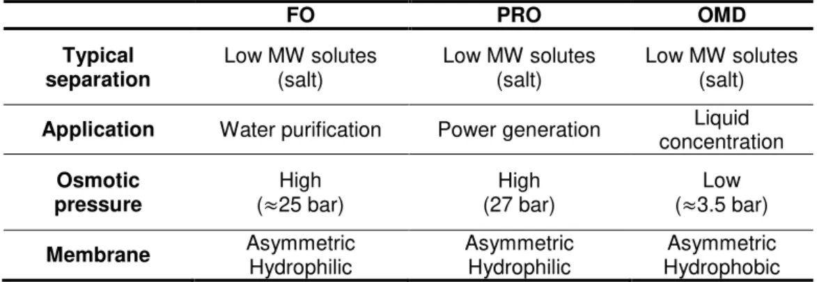
4 Table 1 - Summary of the main properties of the osmotically-driven separation processes (Khayet,
et al., 2011; Achilli, et al., 2009; Qin, et al., 2012; Gostoli, 1999)
FO PRO OMD
Typical
separation Low MW solutes (salt)
Low MW solutes (salt)
Low MW solutes (salt)
Application Water purification Power generation Liquid concentration
Osmotic
pressure (≈25 bar) High
High (27 bar)
Low (≈3.5 bar)
Membrane Asymmetric
Hydrophilic
Asymmetric Hydrophilic
Asymmetric Hydrophobic
In the FO process is not necessary to apply pressure to the system, the water will flow to the
permeate side due to an osmotic pressure differential (∆π) across the membrane, caused by
the concentrated solution in the permeate side (see Figure 2). Different names are used to
name this solution; in this work the term draw solution will be used. So in this process the water
will flow across the semi-permeable membrane from a saline stream into the highly
concentrated draw solution, diluting it, thus it is possible to effectively separate the water from
the saline feed water stream. The water is subsequently extracted from the dilute draw solution
by removing the solute. In order to achieve an effective FO desalination, the draw solute must
have a high osmotic efficiency (namely high solubility in water and low molecular weight), as to
be easy and inexpensively separated to yield potable water, without being consumed in the
process (Cath, et al., 2006; Chay; McCutvheon, et al., 2006).
Figure 2- Solvent flows in FO and RO. For FO, ∆P is approximately zero and water diffuses to the
more saline side of the membrane. For RO, water diffuses to the less saline side due to hydraulic pressure (∆P>∆π) (Cath, et al., 2006).
5 Table 2- The Comparisons between RO and FO (Liu, et al., 2009)
Sort Reverse Osmosis Forward Osmosis
Driven
pressure High hydraulic pressure Osmotic pressure difference
Water
recovery 30%~50% At least ~75%
Environment effect
Harmfully
(concentrated brine) Friendly
Membrane
fouling Seriously Hardly
Modules Compression resistance Without particular desire
Application Normal separation system
Temperature-sensitive system; Pressure sensitive
system; Renew energy; Control release of drug
Energy Consumption
High energy expenditure (1.6 - 3.02 kW.h.m-3) (Triwahyudi,
2007; Avlontis, et al., 2003)
Low energy demand (0.24 kW.h.m-3, low temperature, 1.5M Feed)
(Triwahyudi, 2007)
Equipments
High-pressure pumps; Energy recovery unit; Resistant high pressure
pipelines; High investment in equipments
Low investment equipment
2.1. Overall advantages of Forward Osmosis
FO has a range of potential benefits, mainly due to the low hydraulic pressure required,
holding a promise of low energy consumption, and so a decrease in operation costs. This is one
of the most attractive points of FO, especially under the growing energy crises. However, this
aim can only be achieve by choosing the appropriate draw solution and its regeneration method
(Zhao, et al., 2012; Elimelech, et al., 2011; Qin, et al., 2012; Elimelech, 2006).
Recent studies have demonstrated that membrane fouling in FO is relatively low (Achilli, et
al., 2009), more reversible (Mi, et al., 2010) and can be minimized by optimizing the
hydrodynamics (Lee, et al., 2010). Therefore, avoiding the additional costs required to clean the
membrane by chemical cleaning agents (unlike RO) (Lee, et al., 2010). Additionally, a variety of
contaminants can be effectively rejected via the FO process (Cartinella, et al., 2006; Cath, et al.,
6 FO also has the potential to help achieve high water flux and high water recovery due to the
high osmotic pressure gradient across the membrane. High water recoveries could help reduce
the volume of desalination brine, which is a major environmental concern for current
desalination plants, particularly for inland desalination (Zhao, et al., 2012).
Furthermore, in the fields of liquid food and pharmaceutical processing, FO has the
advantage of maintaining the physical properties (e.g. colour, taste and aroma) of the feed
without deteriorating its quality since the feed is not pressurized or heated (Jiao, et al., 2004;
Yang, et al., 2009). For medical applications, FO can assist in the release of drugs with low oral
bioavailability (e.g. poor solubility) in a controlled manner by osmotic pumps (Shokri, et al.,
2008). Due to having such a diverse range of potential benefits, FO has been proposed for use
and investigated in a variety of applications.
2.2. System thermodynamics
The mathematical description of permeation in membranes is based in thermodynamics, that
the driving forces of pressure, temperature, concentration, and electromotive force are
interrelated and that the overall driving force producing movement of a permeant is the gradient
in its chemical potential. So the flux, Q, of component i, is described by
Q= −SQ.TUTWV (3)
Where X QZXY the gradient in chemical potential of component i and SQ is a coefficient of
proportionality linking this chemical potential driving force with flux (Baker, 2000; Wijmans, et al.,
1995). Restricting the chemical potential into driving forces generated only by concentration and
pressure gradients, the chemical potential can be written as
7 Where Q is the molar concentration (mol.dml-3) of component i, ]Q is the activity coefficient
linking concentration with activity, p is the pressure, and `Q is the molar volume of component i.
In incompressible phases, such as a liquid or a solid membrane, volume does not change with
pressure. So equation (4) can be integrated with respect to concentration and pressure, giving
Q= Q°+ JK [ \]Q Q^ + bQ\a − aQ°^ (5)
Where Q°is the chemical potential of pure at reference pressure, aQ° (Wijmans, et al., 1995).
In general the reference pressure, aQ° is defined as the saturation vapor pressure of , aQdef.
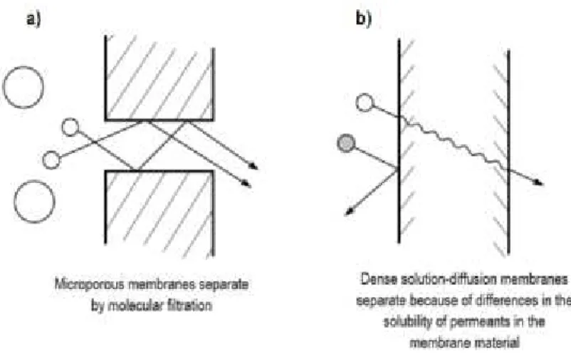
To better describe the mechanism of permeation there are two models, the solution-diffusion
model and the pore-flow model, which are illustrated in Figure 3. In the first model, the
permeants dissolve in the membrane material and then diffuse through the membrane down a
concentration gradient. The permeants are separated because of the differences in solubilities
of the materials in the membrane and the differences in the rates at which the materials diffuse
through the membrane. And in the second model, the permeants are transported by
pressure-driven convective flow through tiny pores. Separation occurs because one of the permeants is
excluded (filtered) from some of the pores in the membranes through which other permeants
move (Baker, 2000; Wijmans, et al., 1995).
Figure 3- Molecular transport through membranes can be described by a flow through permanent pores (a) or by the solution-diffusion mechanism (b) (Baker, 2000)
These two models differ in the way the chemical potential gradient in the membrane phase is
8 membrane is uniform and that the chemical potential gradient across the membrane is
expressed only as a concentration gradient. And in the case of the pore-flow model, the
concentration of solvent and solute within the membrane are uniform and that the chemical
potential gradient across the membrane is expressed only as pressure gradient (Wijmans, et al.,
1995).
The solution-diffusion model was previously proven to have a good agreement between
theory and experiment to describe the water transport in FO and RO (Wijmans, et al., 1995). To
define this model, two assumptions have to be made. The first one is that the fluids on either
side of the membrane are in equilibrium with the membrane material at the interface. The
second assumption is that the pressure within the membrane is uniform (at a high pressure
value, ag) and the chemical potential gradient across the membrane is expressed only as a
smooth gradient in solvent activity ]Q Q (as shown in Figure 4).
Figure 4- Pressure driven permeation of one-component solution through a membrane according to the solution-diffusion transport model, where -= (-=h- (Baker, 2000)
Therefore, because no pressure gradient exists within the membrane, the water flux in the
FO and RO processes can be described in terms of chemical potential by forces only generated
9 Figure 5 - Chemical potential, pressure, and solvent activity profiles through an osmotic membrane following the solution-diffusion model. The pressure in the membrane is uniform and equal to the
high-pressure value, so the chemical potential gradient within the membrane is expressed as concentration gradient (where -= (-=h-) (Baker, 2000)
So the flux of component i (Q)can be described by the following equation:
Q= −FGijVV.TjTWV (6)
Where, J is the ideal gas constant, K is the temperature, and SQ is a coefficient of
proportionality linking this chemical potential driving force. Equation (6) has the same form as
Fick’s Law, in which the term JKSQ⁄ Q can be replaced by the diffusion coefficient, Q. So
10
Q=
lV\jVm\n^ojVp\n^^
q (7)
In order, to achieve a general equation describing the water transport in the RO and FO
processes, from the definition of chemical potential, it is assumed that the fluids on either side of
the membrane are in equilibrium with the membrane material at the interface. Thus, equating
the chemical potential in the solution and membrane phase at the feed-side interface of the
membrane, gives
Qr = Qr\n^ (8)
Substituting the expression for the chemical potential, from equation (5), gives
Q°+ JK lnu]Qir Qrv + bQuag− aQdefv = Q°+ JK ln w]Qr\n^ Q\n^x + bQr\n^uag− aQdefv (9)
Which leads to
lnu]Qir Qrv = ln w]Qr\n^ Q\n^x (10)
And thus
Qr\n^ =
yVr\n^z
yVr\n^ Qr (11)
Hence, defining a sorption coefficient {Qi as
{Qi=yyVr
Vr\n^ (12)
11
Qr\n^= {Qi. Qr (13)
In the RO process, a pressure difference exists at the permeate interface from ag within the
membrane to aq in the permeate solution. Thus, equating the chemical potentials across this
interface obtains
Qp = Qp\n^ (14)
Substituting as before, for the chemical potential of an incompressible fluid, it leads to
lnu]Qip Qpv = ln w]Qip\n^ Qp\n^x +|V\}FGro}p^ (15)
Rearranging and substituting for the sorption coefficient, {Qi, gives the expression
Qp\n^= {Qi. Qp. Ya ~
o|V\}ro}p^
FG • (16)
The expressions for the concentrations within the membrane at the interface in equations
(13) and (16) can now be substituted into the Fick’s Law expression, equation (7), to yield
Q=lV€V
z
q • Qr− Qp Ya ~o|V\}FGro}p^•‚ (17)
This equation can be simplified assuming that the membrane as high permeability, so
Q. {Qq⁄ ≫[ „. {„q⁄[ (… refers to the salt component). Consider first, the water flux at the point
which the applied hydrostatic pressure balances the water activity gradient (osmotic equilibrium,
Figure 5 C) the flux of water across the membrane is zero. So equation (17) becomes
Q=lV€V
z
q • Qr− Qp Ya ~
o|V\}ro}p^
FG •‚ (18)
12
Qp = Qr Ya ~|VFG\∆†^• (19)
At hydrostatic pressures higher than ∆ , equations (17) and (19) can be combined to yield
Q=lV€V
zj Vr
q •1 − Ya ~
o|V\∆}o∆†^
FG •‚ (20)
A trial calculation shows that the term −bQ\∆a − ∆ ^ JK⁄ is small under the normal RO
conditions. So it can be used the simplification 1 − exp \Y^ → Y as Y → 0 and the equation (20)
becomes
Q=lV€V
zj
Vr|V\∆}o∆†^
qFG (21)
This equation can be simplified, giving the general equation that describes the water
transport in FO and RO:
M= •. \∆Ž − ∆ ^ (22)
Where M is the water flux, • the water permeability constant of the membrane and ∆Ž is the
applied pressure. But, in the case of FO, ∆Ž is zero, and the driving force only depends on ∆ .
So for the FO process, the water flux is defined by
M= •. ∆ (23)
The water permeability constant (A) is dependent on the semipermeable membrane
thickness, solubility of water into the membrane and diffusivity of water within the membrane
(Kim, et al., 2008).
A simplified equation for the salt flux, •, through the membrane also, can be derived, starting
13
C= •. \B•g− B•q^ (24)
Where • is the salt permeability constant (• =ldq€dz).
From equations (23) and (24), the ratio between • M⁄ can be derived to give the following
relationship (where ∆ = . O. J. K) (Xiao, et al., 2011):
‘d
‘I=
’ “.
”
•.–.F.G (25)
This relationship demonstrates that the • M⁄ ratio is directly dependent on the membrane
separation characteristics (• •⁄ ) for a given operating condition ( . O. J. K~ constant).
From this application of the solution-diffusion model, it can be obtained a measure of the
ability of the membrane to separate the salt form the feed solution, the rejection coefficient, J,
which is defined as
J = ˜1 −jdp
jdr™ . 100% (26)
2.3. Concentration polarization and fouling in osmotic processes
The main problem in membrane processes is the decline of flux as a function of filtration time
due, most importantly, to concentration polarization (remaining constant once established) and
membrane fouling (worsening as a function of time). They cause extra resistances on top of the
membrane resistance and thus slow down the transport. These phenomena’s are illustrated on
Figure 6. Fouling refers to the accumulation of retained molecules or particles in the pores of
the membrane or at the membrane surface. Concentration polarization (CP) refers to the effect
of the build up of solute on the membrane surface (on the feed side) causing a diffusive solute
flux from the membrane surface towards the feed, forming a kind of “dynamic” membrane,
14 Figure 6- Flux decrease as function of time due to the combined effect of fouling and
concentration polarization (Crespo, et al., 2005)
In the FO process, problems can occur on both sides of the membrane due to CP, so it is
required special membranes for these processes. Consequently membranes with a
conventional asymmetric structure (active layer on a porous support layer), can suffer from two
types of CP phenomena, external CP and internal CP. Both of them can be manifested as a
dilutive or concentrative CP (Cath, et al., 2006; Chou, 2010). Generally, external CP occurs at
the surface of the active layer of the membrane and internal CP occurs within the porous
support layer of the membrane (Zhao, et al., 2012).
a. External concentration polarization
As in pressure-driven membrane processes, external CP in FO occurs at the surface of the
membrane active layer. The difference is that only concentrative external CP can take place in a
pressure-driven membrane process (e.g. RO), while both concentrative and dilutive external CP
may occur in an osmotically driven membrane process depending on the membrane orientation.
The solute build up on the membrane active layer surface, due to the feed solution, is called
concentrative external CP. Simultaneously, the draw solution in contact with the permeate side
of the membrane is being diluted at the permeate-membrane interface by the permeating water.
This is called dilutive external CP. Both of the phenomena reduce the effective osmotic driving
force and the water flux. The undesirable effect of external CP can be minimized by increasing
flow velocity and turbulence at the membrane surface (Cath, et al., 2006; Liu, et al., 2009;
15 Knowing the overall effective osmotic driving force is important to determine the flux
performance in FO. Therefore is important to determine the concentration of the feed/draw on
the membrane surface. In the case of concentrative external CP is necessary to quantify the
feed at the active layer surface. This is not an easily measurable quantity, though it can be
calculated from experimental data using boundary layer film theory (McCutcheon, et al., 2006).
Determining the membrane surface concentration begins with the calculation of the Sherwood
number for the appropriate flow regime. In general, the Sherwood (›ℎ ) number is related to the
Schmidt (› ) and Reynolds (J ) numbers as follows (McCutcheon, et al., 2006; McCutvheon, et
al., 2006; Baker, 2000; Mulder, 1996; Cath, et al., 2012):
›ℎ = •. J ž› j. wTŸ
ix T
(27)
Where, X is the hydraulic diameter (depends on the geometry of the system) and S is the
length of the channel. The values •, , , X depend on the system geometry, type of fluid
(Newtonian and non-Newtonian) and flow regime. The mass transfer coefficient, ¡, is related to
›ℎ by
¡ =C .ld
TŸ (28)
Where • is the solute diffusion coefficient. The mass transfer coefficient is then used to
calculate what is called the concentrative external CP modulus:
†¢,n
†¢,£ = Ya w
‘I
¤¢x (29)
Where M is the experimental permeate water flux, ¡¥ is the mass transfer coefficient on the
feed side, and ¥,¦ and ¥,ž are the osmotic pressures of the feed solution at the membrane
surface and in the bulk, respectively.
In the case of dilutive external CP, the modulus can be defined as above, except that in this
16
†§,n
†§,£ = Ya w−
‘I
¤§x (30)
Here, l,¦ and l,ž are the osmotic pressures of the draw solution at the membrane surface
and in the bulk, respectively.
To model the flux performance of the FO process in the presence of external CP, some
corrections has to be made to M= •. \∆Ž − ∆ ^ (22equation (23). This equation predicts flux as
a function of driving force, without taking into account the concentrative or dilutive external CP,
which may be valid only if the permeate flux is very low. When flux rates are higher, this
equation must be modified to include both the concentrative and dilutive external CP
(McCutcheon, et al., 2006):
M= • ~ l,ž. exp w−¤‘I§x − ¥,ž. Ya w‘¤I¢x• (31)
However, no dense symmetric membranes are in use today for osmotic processes, due to
the low hydraulic pressure used in FO. So, membrane fouling caused by external CP, has
milder effects on water flux, comparing with the effects on pressure-driven membrane
processes (Cath, et al., 2006; Gray, et al., 2006; McCutvheon, et al., 2006). Therefore the
usefulness of this particular flux model is limited.
b. Internal concentration polarization
When a composite or asymmetric membrane consisting of a dense separating layer and a
porous support is used in FO, two phenomena can occur depending on the membrane
orientation. If the porous support layer of the asymmetric membrane faces the feed solution, a
polarized layer is established along the inside of the dense active layer as water and solute
propagate the porous support layer. This phenomenon, referred to as concentrative internal
concentration polarization (illustrated in Figure 7 (b)), is similar to concentrative external CP,
except that takes place within the porous layer. If the membrane is run in the opposite
17 facing the draw solution), when the water permeates the active layer, the draw solution within
the porous substructure becomes diluted. This phenomenon is called dilutive internal CP
(illustrated in Figure 7 (c)). These phenomena cannot be controlled by cross-flow since they
occur within the membrane structure (McCutvheon, et al., 2006).
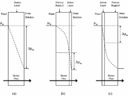
Figure 7 – Illustrations of driving forces profiles, expressed as water chemical potential,
@., for osmosis several membrane types and orientations. (a) A symmetric dense membrane. (b)
An asymmetric membrane with the porous support layer against the feed solution; the profile illustrates concentrative internal CP. (c) An asymmetric membrane with the dense layer against the
feed solution; the profile illustrates dilutive internal CP. The actual (effective) driving force is represented by ∆@.. External CP effects on the driving force are assumed to be negligible in this
figure (McCutvheon, et al., 2006).
From Figure 8, it can be seen that the osmotic pressure difference between the bulk feed
and bulk draw solution (∆ ž¨q¤) is higher than the osmotic pressure difference across the
membrane (∆ ¦) due to external CP and that the effective osmotic pressure driving force
18 Figure 8- Illustration of osmotic driving force profiles for osmosis through several membrane types and orientations, incorporating both internal CP and external CP. (a) Symmetric dense membrane; the profile illustrates concentrative and dilutive external CP. (b) An asymmetric membrane with the dense active layer against the draw solution (PRO mode); (c) An asymmetric
membrane with the porous support layer against the draw solution (FO mode); the profile illustrates dilutive internal CP and concentrative internal CP. Key: 4*, is the bulk draw osmotic pressure, 4*,( is the membrane surface osmotic pressure on the draw side, 45, is the bulk feed osmotic pressure, 45,( is the membrane surface osmotic pressure on the feed side, 45,- is the effective osmotic pressure of the feed in PRO mode, 4*,- is the effective osmotic pressure of the
draw solution in FO mode, ∆4( is the osmotic pressure difference across the membrane, and ∆4677
is the effective osmotic driving force (McCutcheon, et al., 2006)
The water and solute flux in a FO process can be modelled by coupling the solution-diffusion
model with the diffusion-convection transport in the membrane support layer (Tang, et al., 2010;
McCutcheon, et al., 2006). So, considering the PRO configuration, and applying the
solution-diffusion model to the active layer, gives equation (23)M= •. \∆Ž − ∆ ^ (22) for the water flux
(M), and equation (24) for the salt flux. Both equations considered the difference in
concentration/osmotic pressure between the draw solution and the interface of FO support layer
and active layer. For the solute transport in the support layer, the transport of solute into the
support by convection (MB) and that due to the solute back-transport through the rejection layer
(•) have to be balanced by the solute diffusion away from the support:
MB + •= ©ªªTDTW (32)
Where B is the solute concentration in the porous support layer at a distance Y away from
19 coefficient of solute. In a porous support layer with a porosity of «, ©ªª is related to the solute
diffusion coefficient by ©ªª= «. The boundary conditions for equation (32) are:
• Y = 0, B = B•¨}}¬-®
• Y = [©ªª= [¯
Where [ is the actual thickness of the FO support layer, [©ªª is the effective thickness of the
support layer, and ¯ is the tortuosity of the support layer. Solving equation (32), substituting M
and • with the equations obtained from the solution-diffusion model, gives:
ln ˜Dd°±±m²f³’\D´²eIoDd°±±m²f^ “\†⁄ ´²eIo†d°±±m²f^
Dµ¶¶´³’\D´²eIoDd°±±m²f^ “\†⁄ ´²eIo†d°±±m²f^ ™ =
‘I
¤n (33)
Where ¡¦ is the effective mass transfer coefficient, which takes into account the impact that
the porous support layer has on mass transfer, and it is given by
¡¦=lq¶µµ¶µµ=·q ¸lZ =lC (34)
Where › is the structural parameter, analogous to the boundary layer thickness for external
CP in a typical reverse osmosis process, which is given by
› =·q¸ (35)
Assuming that the osmotic pressure of a solution is proportional to its concentration,
equation (33) can be simplified to:
ln ¹†d°±±m²f³’ “Z
†µ¶¶´³’ “Z º =
‘I
¤n (36)
20
M= ¡¦ln ˜“†“†´²eIµ¶¶´o‘³’I³’™ (37)
For the FO configuration, the flux equation can be similarly derived, giving:
M= ¡¦ln ˜“†“†µ¶¶´´²eI³‘³’I³’™ (38)
c. Membrane fouling
Like CP, membrane fouling is also an important and inevitable phenomenon in all membrane
processes. Lower membrane fouling implies more product water, less cleaning and longer
membrane life, thereby reducing operational and capital costs. However, membrane fouling in
osmotically driven membrane processes is different from that in pressure-driven membrane
processes due to low hydraulic pressure being employed in the former processes.
Membrane fouling in FO was primarily studied by Cath et al. (Cath, et al., 2005; Cath, et al.,
2005), which reported that FO might have the potential of low membrane fouling since no sign
of flux reduction due to fouling was observed in their studies. Lately FO has been used in
OMBR for wastewater treatment mainly due to its low fouling and low energy consumption
(Achilli, et al., 2009), which are the two major problems of membrane bioreactors. Achilli et al.
(Achilli, et al., 2009) tested a submerged OMBR to treat domestic wastewater, with long-term
(up to 28 days) experiments, the results showed that the water flux decline was mainly caused
by membrane fouling. However, the flux could be recovered to approximately 90% of the initial
value though osmotic backwashing. This indicates that membrane fouling does exist in FO,
becoming obvious in long-term operation.
Furthermore, membrane fouling in FO and RO has been compared and is thought to be
quite different from one another in terms of reversibility and water cleaning efficiency (Zhao, et
al., 2012). Lee et al. (Lee, et al., 2010) observed that membrane fouling in FO is almost
completely reversible while it is irreversible in RO. However, they attributed FO fouling to the
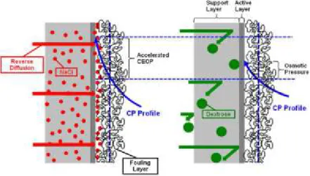
21 draw solution (illustrated in Figure 9). When the draw solution is facing the membrane support
layer, the draw solute accumulates at the surface of the active layer through reverse diffusion,
enhancing the CP layer and reducing the net osmotic driving force. A draw solute with a smaller
hydrated radius (e.g. NaCl) is more readily to cause CEOP compared with one with larger
hydrated radius (e.g. dextrose) (Zhao, et al., 2012). Also, it was reported that FO fouling can be
significantly minimized by increasing the cross flow velocity (Lee, et al., 2010).
Figure 9 – A conceptual illustration of the effect of draw solute reverse diffusion on cake-enhanced osmotic pressure (CEOP) in FO for different draw solutions: a) NaCl and B) dextrose (Lee, et al.,
2010)
Both, CP and membrane fouling are critical inevitable phenomena in FO processes because
they increase the extra resistance of the membrane and thus reduce the overall membrane
permeability. So to improve FO performance, it is necessary to understand these mechanisms.
2.4. Reverse solute diffusion
The reverse diffusion of solute from the draw solution through the membrane to the feed
solution is also inevitable in osmotically driven membrane processes, due to the concentration
differences. Hancok and Cath (Hancock, et al., 2009) suggested that the reverse diffusion of the
draw solute have significant implications on the performance and sustainability of the FO
process. Recent studies have correlated the reverse diffusion of the draw solute to membrane
22 CEOP and increase the fouling layer resistance. Therefore, multivalent ion solutions with lower
diffusions coefficients may be preferable in some specific applications in which high rejection is
desired (Zhao, et al., 2012). However, some multivalent ions (e.g. Ca2+ and Mg 2+) may interfere
with the foulants in the feed solution after reverse diffusion, which is likely to aggravate
membrane fouling (Zou, et al., 2011). Also, multivalent ion solutions may also introduce more
severe internal CP because of their large ion sizes and lower solution diffusion coefficients
(Zhap, et al., 2011). This solute transport is determined by the selectivity of the membrane
active layer, but is independent of the draw solution concentration and the structure of the
membrane support layer (Philip, et al., 2010). This finding has significant implications as it
poses another criterion for the development of a new membrane: high selectivity of the
membrane active layer. Furthermore, employing a multivalent ion solution as the draw solution
may minimize the reverse solute diffusion and thus reduce membrane fouling, but the resultant
higher internal CP and the potentially increased risk of fouling must be considered carefully.
Overall, reverse solute diffusion has been one of the challenges in osmotically driven
membrane processes and it should be fully considered and minimized in the
developments/design of both FO membranes and draw solute (Zhao, et al., 2012).
2.5. Draw solutions
The osmotic pressure difference is the driving force in the FO process. So, the selection of
optimal osmotic agents is one of the key factors for a higher water flux. The main criterions to
select a suitable draw solution are as follows: the solute must have a high osmotic efficiency,
namely high solubility in water and relatively low molecular weight, which can lead to high
osmotic pressures; osmotic agents should ideally be inert, stable, neutral or near neutral pH,
and non-toxic; solute must also be easily and inexpensively separated to yield potable water,
without being consumed in the process (i.e., minimal reverse draw solute diffusion) which may
lower the replenishing cost. Moreover, the draw solutions should not degrade the membrane
23 are crucial for the viability of the process at the municipal scale, and have direct consequence
on the operating costs of a FO plant (Qin, et al., 2012).
Figure 10 shows the daily amount of draw solute that needs to be replenished for a FO
process due to loss through the membrane for three different • M⁄ scenarios. Current FO
membranes could achieve • M⁄ down to around 0.1 g.L-1 for NaCl (Scenario B), which means
that a municipal scale FO plant with the capacity of 100000 m3.d-1 will lose 10000 kg of NaCl on
a per day basis, which need replenishment. From a logistics point of view, Scenario C needs no
further consideration for a municipal scale FO plant, whereas Scenario A is technically not yet
achievable with current FO membranes and for NaCl as the draw solute (Qin, et al., 2012).
Figure 10- Daily requirement of draw solute replenishment (kg/d) as function of water production (m3/d) derived based on equation (25) for the three scenarios: (A) ,/⁄,.=0.01 g.L-1; (B) ,/⁄,.=0.1
g.L-1; and (C) ,/⁄,.=1 g.L-1(Qin, et al., 2012)
Another way of evaluation is to consider the additional operating costs to a FO desalination
plant due to the replenishment for the lost draw solutes for scenarios of various draw solute cost
and • M⁄ Table 3 show different scenarios, with a range of draw solutes prices and a range of
• M⁄ ratios. Typically, costs for various types of draw solutes range between $10.kg-1 and
$100.kg-1 (Lee, et al., 2010), such that commonly available chemicals such as NaCl may be
represented by the $10 per kg cost range, whereas other more specialized chemicals may be
represented by the $100 per kg costs range. It is also assumed that specific low cost draw
24 Table 3 – Additional operating costs to a FO desalination plant for replenishment of lost
draw solutes(Qin, et al., 2012)
Draw solute cost ,/⁄,. (A) ,/⁄,.=0.01 g.L-1 (B)
,/⁄,.=0.1 g.L-1 (C) ,/⁄,.=1 g.L-1
1. 1$.kg-1 0.01 $.m-3 0.1 $.m-3 1 $.m-3
2. 10 $.kg-1 0.1 $.m-3 1 $.m-3 10 $.m-3
3. 100$.kg-1 1 $.m-3 10 $.m-3 100 $.m-3
The range of desalination cost for a municipal scale plant (size > 60000 m3.d-1) is typically
0.5-1$ per m3 of water produced (Karagiannis, et al., 2008). On the basis that the additional
operating cost due to replenishment for lost draw solutes should not exceed 10-20% of the
desalination cost for a municipal scale FO plant, a practical cost limit for draw solute
replenishment may be set as 0.1$.m-3 (i.e. scenario I-(A), I-(B) and II-(A)) (Qin, et al., 2012). Can
be concluded that the economical viability of a municipal scale FO desalination plant it is not
achieved by using expensive draw solute with very low • M⁄ (i.e. scenario III-(A)); neither with a
low-cost draw solute with high • M⁄ (i.e. I-(C)). The discussion here makes clear that both • M⁄
and draw solute cost are crucial factors for selecting an appropriate draw solution for FO
application.
The draw solutions can be composed of different types of solutions and mixtures, like salt
solutions with different concentrations (some examples are showed in Figure 11; also seawater,
Dead seawater and Salt Lake water), mixtures of water and another gas (e.g. sulphur dioxide)
or liquid (e.g. aliphatic alcohols), mixture of gases (e. g. ammonia and carbon dioxide gases)
(McGinnis, et al., 2006), 2-methylimidazole, sodium salts of polyacrylic acid (PAA-Na) (Ge, et
al., 2011), albumin, dendrimers with sodium ions attached to the surface (Adham, et al., 2007),
urea, ethylene glycol (Young, et al., 2011), dextrose (Gray, et al., 2006; Lee, et al., 2010),
ethanol, fructose solution (Kim, et al., 2011), glucose solution, and, glucose and fructose
solution (Cath, et al., 2006; Chay). More specifically for fruit juice concentration application, also
can be used as draw solution, glycerol, cane molasses and corn syrup (Jiao, et al., 2004). In a
new nanotechnological approach, naturally non-toxic magnetoferritin is tested as a naturally
non-toxic solute for draw solutions, which can be rapidly separated from aqueous streams using