doi: 10.1590/0101-7438.2018.038.01.0053
PERFORMANCE COMPARISON OF SCENARIO-GENERATION METHODS APPLIED TO A STOCHASTIC OPTIMIZATION ASSET-LIABILITY
MANAGEMENT MODEL
Alan Delgado de Oliveira*, Tiago Pascoal Filomena
and Marcelo Brutti Righi
Received May 31, 2017 / Accepted November 22, 2017
ABSTRACT.In this paper, we provide an empirical discussion of the differences among some scenario tree-generation approaches for stochastic programming. We consider the classical Monte Carlo sampling and Moment matching methods. Moreover, we test the Resampled average approximation, which is an adaptation of Monte Carlo sampling and Monte Carlo with naive allocation strategy as the benchmark. We test the empirical effects of each approach on the stability of the problem objective function and initial portfolio allocation, using a multistage stochastic chance-constrained asset-liability management (ALM) model as the application. The Moment matching and Resampled average approximation are more stable than the other two strategies.
Keywords: scenario generation, stochastic programing, multistage, ALM.
1 INTRODUCTION
Stochastic programming (SP) is a branch of optimization, in which optimal decisions are made under uncertainty (Birge & Louveaux, 2011). In general, real world problems are characterized by uncertain events modeled with random variables. We associate a collection of random events with a probability space containing a bundle of all possible events with their probabilities. From these concepts, we formalize a generic stochastic optimization problem, as denoted by Eq. (1)
G(x)=max
x∈X
F
f(x, ξ )d F(ξ ), (1)
where f is the objective function that is defined in terms of uncertainty,xis the decision variable defined over the feasible set X ⊂ RI, andξ is a random variable defined by the continuous
*Corresponding author.
cumulative distribution function F : RI → [0,1]. Furthermore,d F represents the probability measure of the probability spaceF for the underlying multivariate stochastic process.
As discussed by Pflug (2001), continuous optimization problems become easier to solve if we reduce them to discrete-state multi-period optimization problems. This logical structure may be seen as a tree model with a non-anticipative decision process, in which dependence relies uniquely on this history and on the probabilistic specification (Dupaˇcov´a et al., 2000; Escudero & Kamesam, 1995). Thus, the decision functions reduce to large decision vectors and, as L¨ohndorf (2016) points out, it may be calculated numerically by either drawing a sample from F or by approximatingF with a discrete distributionFˆ. Using Fˆ instead ofF, we have the following maximization problem:
max x∈X
ξ∈ ˆF
ˆ
φ(ξ )f(x,ξ )ˆ (2)
whereφ(ξ )ˆ is the probability of the mass point inFˆ. If we suppose a uniform distribution forφ,ˆ
the approach in Eq. (2) can be seen as sample average approximation (SAA). Stochastic approx-imation (SA) is another approach to obtain numerical convergence for stochastic optimization problems, which presents a random direction whose origin is usually an objective function’s gradient with a step-size for each iteration (Shapiro et al., 2009).
As the scenario generation methodology becomes a key part of the stochastic optimization pro-cess, the main goal of this study is to compare the performance of different scenario sampling methods, in order to highlight which of them is more appropriated for designing a representative discrete-space model for asset-liability management (ALM) problems regarding the in-sample performance. Many efforts have been made in the scenario generation direction, for instance, by having matched state-space distribution moments (Dupaˇcov´a et al., 2000; Høyland & Wallace, 2001; Høyland et al., 2003), minimizing Wassertein probability metrics (Romisch, 2003; Heitsch & Romisch, 2005; Hochreiter & Pflug, 2007), Latin hypercube sampling (McKay et al., 1979), Voronoi cell sampling (L¨ohndorf, 2016), and Resampled average approximation (de Oliveira et al., 2017), among others.
Wallace (2011) introduce copulas in the definition of moments, but they represent perspectives with essentially distinguished methodologies.
Our intent is not to exhaustively test the sampling methods for ALM, but to outline how, em-pirically, the method may have an impact and produce different outputs. Based mostly on the resulting values of the objective function, as suggested by Kaut & Wallace (2007), we can con-clude that the classical Monte Carlo sampling and Monte Carlo with naive allocation strategy are dominated by the Moment matching and the Resampled average approximation.
The paper is organized as follows. First, we introduce this study’s multistage stochastic chance-constrained ALM model in Section 2. Then, in Section 3, the scenario generation methods are described: Monte Carlo sampling (Section 3.1), the Moment matching sampling (Section 3.2), the Resampled average approximation (Section 3.3) and the benchmark Monte Carlo with naive allocation (Section 3.4). Section 4 describes the generation of the sample paths with other ex-planations on the data and the experiment. A comparison of the results considering the different approaches appears in Section 5. Concluding remarks are in the final section.
2 STOCHASTIC ASSET-LIABILITY MANAGEMENT MODEL
ALM is focused on modeling suitable sample paths for the assets and liabilities of a pension fund, bank, insurance company, or any other institution that dynamically manages and matches risks on both sides of a balance sheet (see e.g. Mulvey & Ziemba, 1998; Zenios & Ziemba, 2006; Hochreiter & Pflug, 2007; Haneveld et al., 2010; Mitra & Schwaiger, 2011; Righetto et al., 2016). In other words, the objective of ALM is to guarantee that liabilities are paid over a multi-period horizon by efficiently managing investment resources (e.g. Ziemba, 2003; Matos et al., 2014). Our study’s model is designed for the pension fund environment. Thus, the fund’s assets must be strategically managed so that the total value of all assets is greater than the fund’s liabilities with high probability, while respecting all constraints, for instance, the fund’s solvency (Bogentoft et al., 2001).
Our stochastic ALM model is based on de Oliveira et al. (2017). Suppose that there is a set of securities denoted byi =1, . . . ,N. The ALM manager has to choose from these investment opportunities, allocating the available wealth in order to afford the liabilities denoted bylt. These decisions occur repeatedly through different time periods, t = 1, . . . ,T. The utility function maximizes the final expected wealth. Thus, the model takes the form of a stochastic and inter-temporal dynamic allocation problem, due to the randomness of the asset prices and the time-dependent nature of the investment and rebalancing decisions.
The investment strategy is designed with three sets of variables. The here-and-now decisions that are taken before the information is revealed, denoted byXit s. This is the position (shares) of asset
ito hold in time periodtand scenarios. The corrective actions, which are made after information revealing, are described by bothBit sandVit swait-and-see variables. They are, respectively, the position (shares) ofi bought and sold during timetand scenarios.
The input data of the optimization model is determined by the continuous random variableξ. This stochastic variable may be discretized by ξit that defines the price of asset i at time t. Additionally, it can take a finite number,s ∈ 1, . . . ,S, of realizations denoted by Pit s. As the asset returns are simulated by stochastic process, detailed in Section 4.1, the price realization
Pit sis defined as a conditional sampling of the random variableξit. Therefore, the realizations forPit sdepend onPit−1s(Shapiro et al., 2009).
The scenario tree is comprised of scenarios ranging from the initial to the final period. A sce-nariokconsists of a set of sequential realizations,{Pi1s,Pi2s, . . . ,Pi T s} ∀s∈ S, of the random variableξit. They must be adapted to the non-anticipative constraints that drive the information unfolding process. For instance, the scenariokis a random vector, generated by aξit realization, which is described asλk(ξit)=(Pi1k, . . . ,Pit k), , ∀i ∈ N. Table 1 presents a summary of the model’s notations.
The model is a multistage stochastic programming model with chance constraints, described below:
max S
s=1 N
i=1
φT sPi T sXi T s (3)
s.t.:
Q=
N
i=1
Pi0Xi0 (4)
Xit s=Xi(t−1)s+Bit s−Vit s, ∀t ∈T,∀i∈ N,∀s∈S (5)
P
N
i=1
ξitXit ≥K(Lt−Ft)
Table 1–Notation Summary.
Sets – Indices
t time index (stage)t=0,1, . . . ,T i index of asset classesi=1, . . . ,N s index of scenarioss=1, . . . ,S
Decision variables
Xit s Number of shares of assetsito hold during timetand scenarios
Bit s Number of shares of assetsito buy during timetand scenarios
Xi0 Number of shares of assetsito hold initially (t=0)
Vit s Number of shares of assetsito sell during timetand scenarios
Random variables
ξit Random price of assetiduring timet
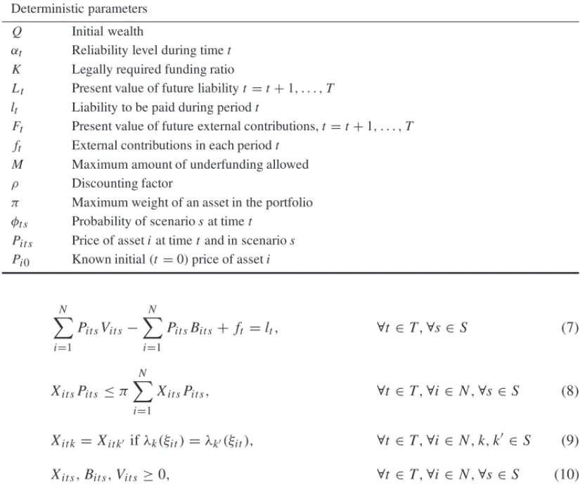
Deterministic parameters
Q Initial wealth
αt Reliability level during timet
K Legally required funding ratio
Lt Present value of future liabilityt=t+1, . . . ,T
lt Liability to be paid during periodt
Ft Present value of future external contributions,t=t+1, . . . ,T
ft External contributions in each periodt
M Maximum amount of underfunding allowed
ρ Discounting factor
π Maximum weight of an asset in the portfolio
φt s Probability of scenariosat timet
Pit s Price of assetiat timetand in scenarios
Pi0 Known initial (t=0) price of asseti
N
i=1
Pit sVit s− N
i=1
Pit sBit s+ ft =lt, ∀t ∈T,∀s∈S (7)
Xit sPit s≤π N
i=1
Xit sPit s, ∀t ∈T,∀i∈ N,∀s∈S (8)
Xit k =Xit k′ ifλk(ξit)=λk′(ξit), ∀t ∈T,∀i∈ N,k,k′∈S (9)
Xit s,Bit s,Vit s≥0, ∀t ∈T,∀i∈ N,∀s∈S (10)
known and deterministic, we can rewrite Xi0s as Xi0,∀s. The numberBi0 of shares bought is equal to the numberXi0(∀i) of shares kept at the end of the initial period. The linear equalities (5) are the share balance constraints. These specify that the number of shares Xit s of asset i during timetand scenariosis equal to the number of sharesXi(t−1)smaintained in the previous period, augmented by the number of purchased sharesBit sminus those soldVit sat timet.
The chance constraints (6) enforce the funding ratio requirements, which represent the long-term relationship between assets and liabilities. The actual funding ratioβt s of a fund during timet and scenariosis computed as:
βt s=
Ft +
N
i=1 Pit sXit s
Lt
, t =1, . . . ,T,s=1, . . . ,S, (11)
whereNi=1Pit sXit sis the current asset value of the pension fund in scenarios. Lt andFt are, respectively, the present value of the future liabilities and contributions discounted byρ:
Lt =
T
j=t
lj
(1+ρ)j−t, Ft =
T
j=t
fj
(1+ρ)j−t.
A value ofβless than 1 signals that the value of the assets may become insufficient to cover future liabilities, so the fund might run into solvency issues in the near future. The two parameters K
andαt define the asset-liability management policy’s risk-aversion. The constraints (6) can be viewed as some sort of VaR constraints, ensuring that the value of the fund is at least equal to
K(Lt−Ft)during each periodtwith a probability at least equal toαt. These maintain the fund’s long-term solvency level.
The model cash flow balance is denoted by the equalities indicated by Eq. (7). The financial inputs are represented by the sales of assets and external contributions, while the financial outputs are payments of liabilities and purchases of assets. The constraint (8) stipulates that no asset can have a weight greater than an upper boundπ. Multistage models have the so-called non-anticipativity condition. This determines that decisions are impacted only by the past, not by the future, i.e. two scenarios with a common history until thetth stage should result in the same decisions until this stage (Carøe & Schultz, 1999). Constraint (9) guarantees that scenarios with the same history present identical asset allocation. A maximum admissible underfunding value is defined through the parameter M. Constraint (10) defines the non-negativity restriction on the decision variables.
3 SCENARIO GENERATION METHODS IN ALM
3.1 ALM with classical Monte Carlo sampling
The traditional method to generate a scenario tree for ALM is through Monte Carlo sampling, with uniformly distributed pseudo-random numbers transformed appropriately into a target dis-tribution (Ubeda & Allan, 1994; Dempster et al., 2011). This approach is an efficient way to represent multi-dimensional distributions (Zenios & Ziemba, 2006). In this study, we gener-ateW1, . . . ,WI random vectors from the standard normal distribution. As Homem-de-Mello & Bayraksan (2014a) note, in this case, the vectorsW1, . . . ,WI are mutually independent; a detail that characterizes this sampling method.
As Monte Carlo is based on the volume of a set distribution for the definition of probability measure, an obvious way to deal with this problem is to increase the number of nodes in the randomly sampled event tree. However, the stochastic program might become computationally intractable due to the tree’s exponential growth rate. This hypothesis is supported, not only by the law of large numbers that guarantees the convergence to a correct value as the number of draws increase, but also by the central limit theorem that offers information about the error magnitude after a finite number of simulations. Hence, the convergence and error estimation of the outputs is directly linked with the number of draws. Indeed, one of the features of Monte Carlo is the form of the standard error, which, for a generic function f, can be defined byσf/√n, withn being the number of draws, andσf the sample standard deviation. The Monte Carlo sampling is also a good choice for integrals in high dimensions, because its convergence rate holds (O(n−1/2)) for any dimension. Glasserman (2003); Rubinstein & Kroese (2016) provide more specific features of Monte Carlo sampling.
According to Kouwenberg (2001), despite the intuitiveness of this approach, the mean and co-variance matrix may not be correctly specified in most nodes of the tree, given that the states are randomly sampled. Thus, the optimizer might choose an investment strategy from erratic or misspecified parameters.
3.2 ALM with Moment matching sampling
The Moment matching approach aims to mitigate the impact of the inconsistencies in the spec-ification, given that it is not possible to reach a full match with misspecified parameters. It also allows the decision maker to determine the output features based on the statistical distribution properties considered relevant.
Furthermore, the literature presents examples in which higher order moments are matched (Høyland et al., 2003). However, it may become very difficult to obtain a solution for non-linear constraints such as skewness and kurtosis. Kouwenberg (2001) and Zenios & Ziemba (2006) also adjust only the first two moments in their analysis. In this study, we construct an event tree that fits the mean and the covariance matrix of the underlying distribution.
In order to fit the first two moments, we use Cholesky decomposition in the same direction as in Høyland et al. (2003). The first step is to generate random vectors from the standard normal distribution, as described in Section 3.1. Then, theI random vectors are transformed to show a given covariance matrix by multiplying the vectors by a lower triangular matrixL of the covari-ance matrix,
W′j =L Wj, =L L′, j=1, . . . ,I, (12)
where we can obtain L by applying Cholesky decomposition. In other words, as Kouwenberg (2001) states, we specify that the average of the disturbances should be zero, and they should have a covariance matrix equal to. Therefore, we denote this matching in Eqs. (13) and (14):
1
S
S
s=1
Wj s=0 ∀j ∈1, ...,I, (13)
1
S−1
S
s=1
Wj sWis =i j ∀j,i∈1, ...,I. (14)
This methodology allows for the generation of different sample paths, which matches the first two moments since the disturbance compose the asset price modeling (see Equations 16 and 17). As in Kouwenberg (2001); Dempster et al. (2011) and L¨ohndorf (2016), it is possible to argue that this sampling approach outperforms other methods, such as Monte Carlo sampling, Wasser-stein distance sampling, or even Latin hypercube sampling. This methodology also enables us to capture unlikely scenarios if we consider higher order moments (Dupaˇcov´a et al., 2000; Høyland & Wallace, 2001).
Unlike Monte Carlo sampling, the Moment matching does not necessarily converge when the number of scenarios is increased. It depends mainly on how much statistical properties are be-ing matched and the distribution features, for example, the smoothness (Kaut & Wallace, 2007). Overspecification and underspecification are also an issue when dealing with the first two mo-ments (Høyland & Wallace, 2001).
3.3 ALM with the Resampled average approximation
The Resampled average approximation is a simulation of many scenario trees, with the average of the initial portfolio taken as the solution (de Oliveira et al., 2017). When we consider several trees, we account for a wide spectrum of variability inherent to the parameters in the optimiza-tion problem. This technique has some similarities to the Resampled efficient frontier method proposed by Michaud & Michaud (2008) to construct portfolios of risky securities. With a math-ematical definition similar to that for the Resampled efficient frontier method for mean-variance optimal portfolios, the ALM Resampled average approximation optimality is the expected value in the solution space of the Monte Carlo ALM financial plan, as presented in Section 3.1. Thus, it may be seen as a reshuffle of the classical Monte Carlo. This methodology could also be adapted to the Moment matching, but the volatility of its results has already been regulated through the adjustment of the second moment. In other words, it is a needless further procedure to miti-gate the risk, which is supposedly one of the main advantages of the Moment matching when compared to the classical Monte Carlo sampling.
This sampling technique is applied and described in detail by de Oliveira et al. (2017). Addi-tionally, this approach can be viewed as a particular case of one of the algorithms discussed by Homem-de-Mello & Bayraksan (2014a), in which the stopping criteria is predefined by the num-ber of runs. The ALM with the Resampled average approximation has four steps. First, we define the number of trees to solve for each parametrization (see e.g. Michaud & Michaud, 2008). The value of these outcomes must be sufficiently large to provide stable portfolio allocations, while being small enough to ensure that the approach does not become computationally prohibitive. After defining the number of instances, the second step is to generate the scenarios for each tree according to the ALM model. In Step 3, we solve each corresponding optimization problem to optimality. In Step 4, we evaluate the results based on the optimal solutions of the trees. The average of the initial allocation portfolio of all simulations is then the model solution. It is distin-guished from SAA because of the number of scenario trees that are solved. In the SAA, a unique scenario tree is generated and solved. In this case, the expectation is applied on the decisions from the next stage. Unusually, the Resampled average approximation gives origin and solves an arbitrary number of unrelated scenario trees with the same topology, but for distinct scenarios. After that, the expectation is taken from these independent instances.
3.4 ALM with the Monte Carlo with naive allocation strategy
In ALM, banks have already used this rule to make their portfolios in the 1960s (Cohen & Hammer, 1967). Furthermore, pension funds also adopted this policy in the 1980s (Harrison & Sharpe, 1983), and the USA Pension Benefit Guaranty Corporation had followed this rule. Al-though the Monte Carlo with naive allocation, or the 1/N portfolio, might provide good returns, they may not be able to meet the legal requirements and cash balance constraints. Additionally, Zenios & Ziemba (2007) show that, as the naive allocation is unable to incorporate new informa-tion, stochastic programming can outperform it for ALM. Fleten et al. (2002) also compared the Fixed-Mix strategy with the multistage stochastic linear programming, verifying the superiority of its model over the Fixed-Mix approach. We consider the 1/N naive policy version for our tests as the benchmark for other sampling methods. We define our naive allocation as an equally distributed portfolio, described in Eq. (15):
Xi0= Q
N ·
1
Pi0
i =1, . . . ,N. (15)
Therefore, we use this popular investment policy with the classical Monte Carlo sampling, de-fined in Section 3.1, in order to settle a comparative level to other methods simulated. Even with the investment policy defined, we have to guarantee that constraints (4)−(10) are respected in this strategy. Therefore, in the simulations executed at Section 4, we set the funding ratio to one. Thus, in the beginning of the simulation’s time horizon, the pension fund has the all necessary wealth to afford the liabilities until the final time period.
4 SIMULATION
First we introduce, in Section 4.1, arbitrage-free continuous-time stochastic processes used to simulate prices at a discrete set of dates (Glasserman, 2003). We adopt the Geometric brownian motion model (GBM) and the Cox-Ingersoll-Ross model (CIR), which is a single-factor term structure model. These stochastic processes are adapted to the scenario tree topology. Then, in Section 4.2, the scenario tree structure is described.
4.1 Generating sample paths
We generate the scenario trees by asset prices realization sampling. The asset prices follow cor-related stochastic differential equations (SDEs). We use the GBM for stock prices (Neftci, 1996; Duffie, 2001):
dξ1t =µξ1tdt+σ ξ1td W1t. (16)
Thus, there is a GBM for each stock. For the price of a fixed income asset, we use the Cox-Ingersoll-Ross term structure model (Cox et al., 1985):
dξ2t =α(µ−ξ2t)dt+
ξ2tσd W2t, (17)
its meanµat speedα. The diffusion functionξ2tσ2is proportional to the interest rateξ2t and ensures that the interest rate is always positive.
The total of succeding nodes for each scenarios at timet (defined by Table 2) are available to describe the conditional distribution of these random variables in a particular node at timet−1. We define the disturbanceWj sas the realization in nodesfor the jth element of the vectorW. The model maximizes the expected wealth of an ALM problem applied to a pension fund, as defined generically in Eq. (1) respecting a set of restrictions.
We use only broad stock or bond indexes that cause arbitrage in cases of very poor approximation of the assets’ underlying distribution on the stochastic programming tree (Kouwenberg & Zenios, 2006). We use just two stock broad indexes and a floating rate fixed income instrument with long-only positions, without any complex asset. We also present a large number of scenarios for each tree. Thus, in our study settings, the discussion of arbitrage is not critical.
The parameters used in GBM, Eq. (16) are estimated through historical time series data. Those used in CIR, Eq. (17), are estimated using maximum likelihood. These sampled paths are con-ditioned to non-anticipative constraints defined in Eq. (9), following the multistage stochastic framework integrated with the sampling algorithms. We simulate the classical Monte Carlo sam-pling, the Moment matching method, the Resampled average approximation and Monte Carlo with naive allocation, as explained in Section 3.
4.2 Scenario tree simulation
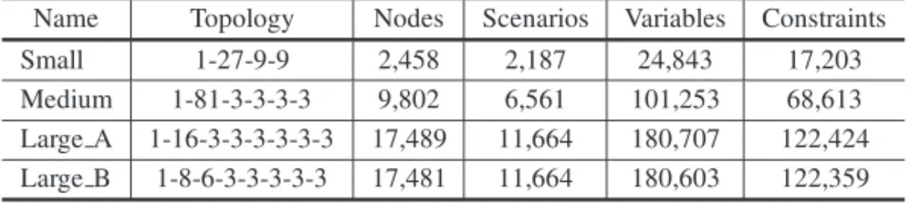
The simulation occurs prior to the optimization process; this methodology is known as the non-recursive method, (see Pflug, 2012). In order to simulate the trees and to study the outputs of the sampling methods, we define three classes of scenario trees that are denoted by small, medium and large according to their number of periods. They have 4, 6 and 8 periods respectively. In each class, we determine a different topology, which produces a distinct number of nodes, scenarios, variables and constraints (Table 2).
Table 2–Classes and Topologies of scenario trees.
Name Topology Nodes Scenarios Variables Constraints
Small 1-27-9-9 2,458 2,187 24,843 17,203
Medium 1-81-3-3-3-3 9,802 6,561 101,253 68,613
Large A 1-16-3-3-3-3-3-3 17,489 11,664 180,707 122,424 Large B 1-8-6-3-3-3-3-3 17,481 11,664 180,603 122,359
distributions of stocks and fixed income assets, calibrated with historical data from January 2012 to November 2016.
We use data from the Brazilian capital market. Equation (16) defines the stock price models, which are calibrated with annualized daily return prices from the Bovespa index (the most liquid stocks in the country) and the Brazilian Small Cap BM&F Bovespa index (stocks with small capitalization). We also have a fixed income asset modeled with Eq. (17) and calibrated with data from the 1-month Brazilian LTN (similar to a T-Bill in the USA) as a proxy for the short-term interest rate. In Table 3, we show the parameters used in the model.
Table 3–CIR and GBM parameters.
Asset Return Annualized (µ) Std. Annualized (σ) Mean Revert. (α)
Fixed Income 0.11297 0.04358 0.14599
Bovespa index 0.13503 0.23486 –
Small Cap index 0.07426 0.17716 –
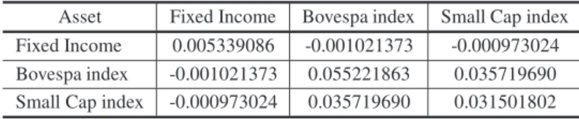
The covariance matrixtakes the variance and covariance among Fixed Income, Bovespa index, and Small Cap index as inputs for Eq. (12) in the Moment matching sampling. In Table 4, we present the covariance matrixobserved from the data.
Table 4–Covariance Matrix for the experiments.
Asset Fixed Income Bovespa index Small Cap index Fixed Income 0.005339086 -0.001021373 -0.000973024 Bovespa index -0.001021373 0.055221863 0.035719690 Small Cap index -0.000973024 0.035719690 0.031501802
In the Monte Carlo with naive allocation approach, we take the initial wealth and allocate it uniformly between the financial assets, as defined in Eq. (4). This position is fixed until the last period. In each period, we calculate the financial value of the portfolio and discount its liabilities. Monte Carlo with naive portfolio is not rebalanced in any time period. Thus, the final expected value of wealth is the sum of the net financial value of the portfolio multiplied by its probability of occurrence, similar to Eq. (3). Even though the Monte Carlo with naive allocation is not a sampling method, we take it into account as an element of comparison for our analysis.
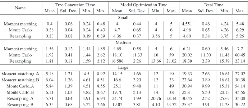
Intel Core i7-4510U 2GHz CPU and with 8GB of RAM. In Table 5, we report each class and method’s computational times (mean and standard deviation) in seconds to solve a single tree.
Table 5–Times elapsed for scenario generation and optimization.
Name Tree Generation Time Model Optimization Time Total Time Mean Std. Dev. Min. Max. Mean Std. Dev. Min. Max. Mean Std. Dev. Min. Max.
Small
Moment matching 0.4 0.06 0.24 0.48 4 0.44 4 5 4.551 0.46 4.24 5.48 Monte Carlo 0.28 0.04 0.24 0.43 4.7 0.65 4 6 4.98 0.65 4.26 6.29 Resampling 0.23 0.02 0.19 0.29 4.36 0.37 3.56 5 4.60 0.38 3.75 5.25
Medium
Moment matching 1.56 0.12 1.44 1.85 4.65 0.58 4 6 6.21 0.60 5.46 7.7 Monte Carlo 1.92 0.41 1.44 2.62 18.10 11.33 10 59 20.02 11.30 11.48 60.45
Resampling 1.81 0.18 1.59 2.12 16.586 2.26 13.66 21.02 18.39 2.39 15.39 23.14 Large
Moment matching A 5.18 1.21 4.5 8.92 14.15 1.66 12 19 19.33 2.63 16.61 27.92 Moment matching B 6.04 1.26 4.61 8.51 16.6 3.20 12 23 22.64 3.89 16.61 30.38 Monte Carlo A 5.84 1.39 4.51 8.55 25.1 9.48 11 49 30.94 9.99 15.51 54.14 Monte Carlo B 6.11 1.03 4.82 8.67 19.70 5.13 14 38 25.81 5.50 20.13 45.56 Resampling A 5.71 0.64 4.91 6.94 24.74 1.99 20.76 28.14 30.45 2.52 25.67 35.08 Resampling B 6.35 0.68 5.22 7.66 19.02 3.81 4.10 23.32 25.37 3.91 11.28 30.72
Based on Table 5, we notice that, on average, the computational time to solve a single tree is between 4 and 61 seconds. For the Resampled average approximation, the computational experiment can be taken from 7.5 to 51 hours to be completed: 6,000 trees must be computed for each instance. For the other three methods, the average time has to be multiplied by 20, which is the number of simulations to finish each experiment. The Monte Carlo with naive allocation strategy is not considered on Table 5 because it does not demand much computational effort. Next, we present and describe the results from the simulations.
5 RESULTS
Our results focus on the stochastic programming in-sample stability (Kaut & Wallace, 2007). The in-sample stability is evaluated by generating different scenarios for each tree and comparing how stable the problem’s objective function and solution are. Thus, we analyze the stability of the sampling methods from two different perspectives: objective function and initial portfolio allocation. Dempster et al. (2011) argue that the initial portfolio allocation criterion is not often used in the literature, because of the potential for a flat plateau objective function. However, as our scenarios might have sampling error, we conducted the analyses from both perspectives. We focus on the expectation and volatility of both the objective function and initial portfolio allocation. The results of the objective function and initial portfolio allocation are presented in Tables 6 and 7, respectively.
Table 6–Objective function statistical outputs.
Name Mean Std. Dev. Min. Max.
Small
Resampling 714,114.47 2,805.67 708,800.98 720,443.70
Moment matching 629,656 7,341.04 619,961 642,192
Naive allocation 814,619.86 30,153.65 762,498.94 864,254.46
Monte Carlo 712,815.40 22,927.45 672,949 756,231
Medium
Resampling 1,065,780.19 3,850.40 1,056,652.26 1,073,008.54
Moment matching 711,529.65 8,698.65 695,761 727,839
Naive allocation 1,136,827.87 26,529.07 1,072,786.30 1,184,755.13 Monte Carlo 1,074,340.85 20,485.86 1,028,342 1,106,371
Large
Resampling A 1,584,145.66 18,498.18 1,554,806.82 1,633,666.16 Resampling B 1,549,304.86 13,994.94 1,526,511.44 1,572,683.32
Moment matching A 828,987 21,964.05 795,107 873,140
Moment matching B 837,172.05 25,982.62 798,804 881,010 Naive allocation A 1,564,422.42 68,972.70 1,469,548.25 1,736,670.72 Naive allocation B 1,625,050.78 117,436.33 1,487,900.62 1,902,890.73 Monte Carlo A 1,586,488.10 137,887.48 1,391,047 1,923,511 Monte Carlo B 1,531,394.65 128,454.55 1,267,510 1,772,048
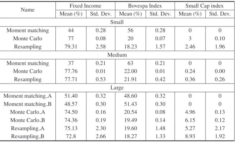
Table 7–Initial allocation of decision variables (%).
Name Fixed Income Bovespa Index Small Cap index
Mean (%) Std. Dev. Mean (%) Std. Dev. Mean (%) Std. Dev. Small
Moment matching 44 0.28 56 0.28 0 0
Monte Carlo 77 0.08 20 0.07 3 0.10
Resampling 79.31 2.58 18.23 1.57 2.46 1.96
Medium
Moment matching 37 0.21 63 0.21 0 0
Monte Carlo 77.76 0.01 22.00 0.01 0.24 0.00
Resampling 77.71 0.53 21.91 0.42 0.36 0.26
Large
Moment matching A 51.40 0.32 48.60 0.32 0 0
Moment matching B 48.57 0.30 51.43 0.30 0 0
Monte Carlo A 74.50 0.16 20.54 0.08 4.96 0.13
Monte Carlo B 74.36 0.19 19.49 0.14 6.15 0.12
Resampling A 75.13 2.30 19.60 1.48 5.27 2.17
Furthermore, we notice that the average value of the objective function in the Moment matching is 11.66% and 12.19% lower compared, respectively, to the Monte Carlo sampling and to the Resampled average approximation in the small trees. This difference increases in large trees. In the medium class, it is 33.77% and 33.23% lower. For the large class, it becomes 47.74% and 47.66% for the instance Large A and 45.33% and 45.96% for Large B. We believe that this happens due to the adjustment in the tree. When the second moment is adjusted, volatility might be reduced and, thereby, the extreme scenarios (good or bad) are probably taken out of the sampling. Clearly, the Resampled average approximation and the Moment matching dominate the other two methods in terms of the stability of the objective function.
In relation to the initial asset allocation (Table 7), the investment in fixed income is quite similar for the Monte Carlo sampling, the Moment matching and Resampled average approximation. The main difference is that the Moment matching never allocates capital in the Small Cap index. The volatility of the Monte Carlo sampling and the Moment matching are also similar. The Re-sampled average approximation and Monte Carlo sampling present similar allocations, but very different allocation volatilities. However, given that the Resampled average approximation takes expectations from the Random sampling, the volatility of the allocation is close to zero. This is consistent with the methodology, as the Resampled average approximation mitigates volatility using the expected value from many trees, making the initial allocation smoother. Notice that, for the Monte Carlo with naive approach, by design, the initial allocation is constant among the assets, so we omit the results from Table 7.
In terms of the stability of the objective function, the Moment matching and Resampled average approximation dominate both Monte Carlo sampling and with naive allocation strategy. The sta-bility of the initial allocation is similar for the Monte Carlo sampling and the Moment matching. Furthermore, the initial allocation’s low volatility, presented by the Resampled average approx-imation, is a result of taking an average of averages. Considering not only the mixed results obtained on the initial asset allocation stability but also the argument of Dempster et al. (2011), that a flat plateau can make many different allocations, resulting in very close values of objective functions, we can focus on the objective function stability results. Then, clearly, the Moment matching and Resampled average approximation present more stable solutions.
6 CONCLUSIONS
In this study, we provided an empirical discussion of the differences among methods to generate scenario trees for stochastic programming in ALM. We examined Monte Carlo sampling, Mo-ment matching, the Resampled average approximation and Monte Carlo with naive allocation strategy as the benchmarks.
scenario trees. It should be arranged so that it is smaller than or equal to the number of sce-nario tree branches in order to guarantee the absence of arbitrage conditions (Geyer et al., 2010). Therefore, the model becomes computationally intractable very quickly when the number of as-sets rises, since they define a lower bound to number of branches, which can be used to calculate the exponential growth of scenario tree (G¨ulpinar et al., 2004).
The simulations are assessed by in-sample point of view. Thus, the best approximation is the one that minimizes the error between the “true” objective value and the optimal scenario generation method objective value (Kaut & Wallace, 2007). Considering the obtained results of the objective function, we can conclude that the Moment matching and the Resampled average approximation are more efficient in terms of in-sample stability, when compared to Monte Carlo sampling and Monte Carlo with naive allocation. For the initial portfolio allocation, the stability of the Mo-ment matching and Monte Carlo sampling are similar and dominated by the Resampled average approximation. However, the low volatility of the Resampled average approximation is a result of taking an average of averages. Taking all the results into account, the Moment matching and the Resampled average approximation are more appropriate for ALM scenario generation.
There are other opportunities for subsequent studies. Scenario reduction and parallel implemen-tation are techniques developed to deal with the curse of dimensionality in stochastic program-ming problems (Beraldi et al., 2010; Dupaˇcov´a et al., 2003; Heitsch & R¨omisch, 2003). For instance, advances in the definitions of bounds (Henrion et al., 2009), different metrics (Heitsch & R¨omisch, 2007) and clustering (Beraldi & Bruni, 2014) have been proposed. The integration of these techniques with different scenario generation methods might present promising results.
ACKNOWLEDGEMENTS
This work was funded by the following Brazilian Research Agencies: CAPES and FAPERGS.
REFERENCES
[1] BENARTZIS & THALERRH. 2001. Naive diversification strategies in defined contribution saving plans.The American Economic Review,91(1): 79–98.
[2] BERALDIP & BRUNIME. 2014. A clustering approach for scenario tree reduction: an application to a stochastic programming portfolio optimization problem.TOP,22(3): 934–949.
[3] BERALDI P, DE SIMONEF & VIOLI A. 2010. Generating scenario trees: a parallel integrated simulation–optimization approach. Journal of Computational and Applied Mathematics, 233(9): 2322–2331.
[4] BIRGE JR & LOUVEAUX F. 2011. Introduction to Stochastic Programming. Springer Sci-ence+Business Media, New York, 2 edition.
[5] BOENDERGCE. 1997. A hybrid simulation/optimisation scenario model for asset/liability manage-ment.European Journal of Operational Research,99(1): 126 – 135. ISSN 0377-2217.
[7] BRADLEYSP & CRANEDB. 1972. A dynamic model for bond portfolio management.Management Science,19: 139–151.
[8] CARINO˜ DR, KENTT, MEYERSDH, STACYC, SYLVANUSM, TURNERAL, WATANABEK & ZIEMBAWT. 1994. The Russel-Yasuda Kasai model: an asset/liability model for japanese insurance company using multistage stochastic programming.Interfaces,24(1): 29–49.
[9] CARØECC & SCHULTZR. 1999. Dual decomposition in stochastic integer programming. Opera-tions Research Letters,24(1): 37–45.
[10] COHENKJ & HAMMERFS. 1967. Linear programming and optimal bank asset management deci-sions.The Journal of Finance,22(2): 147–165.
[11] CONSIGLIG & DEMPSTERMAH. 1998. Dynamic stochastic programming for asset – liability man-agement.Annals of Operations Research,81: 131–161.
[12] COXJC, INGERSOLLJE & ROSSSA. 1985. A theory of the term structure of interest rates. Econo-metrica,53(2): 385–408.
[13] DEOLIVEIRAAD, FILOMENATP, PERLINMS, LEJEUNEM &DEMACEDOGR. 2017. A mul-tistage stochastic programming asset-liability management model: an application to the brazilian pension fund industry.Optimization and Engineering,18(2): 349–368.
[14] DEMIGUELV, GARLAPPIL & UPPALR. 2009. Optimal versus naive diversification: how inefficient is the 1/n portfolio strategy?Review of Financial Studies,22(5): 1915–1953.
[15] DEMPSTERMAH, MEDOVAEA & YONGYS. 2011. Comparison of sampling methods for dynamic stochastic programming. In Stochastic Optimization Methods in Finance and Energy, chapter 16, pages 389–425. Springer Science+Business Media, New York.
[16] DUFFIED. 2001.Dynamic Asset Pricing Theory. Princeton University Press, Princeton.
[17] DUPACOVˇ A´ J, CONSIGLIG & WALLACESW. 2000. Scenarios for multistage stochastic programs. Annals of Operations Research,100(1): 25–53.
[18] DUPACOVˇ A´ J, GROWE¨ -KUSKAN & R ¨OMISCHW. 2003. Scenario reduction in stochastic program-ming.Mathematical Programming,95(3): 493–511.
[19] ESCUDEROLF & KAMESAMPV. 1995. On solving stochastic production planning problems via scenario modelling.TOP,3(1): 69–95.
[20] FERSTLR & WEISSENSTEINERA. 2011. Asset-liability management under time-varying investment opportunities.Journal of Banking and Finance,35(1): 47–62.
[21] FLETENSE, HØYLANDK & WALLACESW. 2002. The performance of stochastic dynamic and fixed mix portfolio models.European Journal of Operational Research,140(1): 37–49.
[22] GEYERA, HANKEM & WEISSENSTEINERA. 2010. No-arbitrage conditions, scenario trees, and multi-asset financial optimization.European Journal of Operational Research,206(3): 609–613.
[23] GLASSERMANP. 2003.Monte Carlo methods in Financial Engineering, volume 53. Springer-Verlag New York, New York, 1 edition.
[25] HANEVELDWKK, STREUTKERMH & VAN DERVLERKMH. 2010. An ALM model for pension funds using integrated chance constraints.Annals of Operations Research,177(1): 47–62. ISSN 0254-5330.
[26] HARRISONJM & SHARPEWF. 1983. Optimal funding and asset allocation rules for defined-benefit pension plans. InFinancial Aspects of the United States Pension System, pages 91–106. University of Chicago Press.
[27] HEITSCH H & R ¨OMISCH W. 2003. Scenario reduction algorithms in stochastic programming. Computational Optimization and Applications,24(2-3): 187–206.
[28] HEITSCHH & ROMISCHW. 2005. Generation of multivariate scenario trees to model stochasticity in power management. InIEEE St. Petersburg Power Tech.
[29] HEITSCHH & R ¨OMISCHW. 2007. A note on scenario reduction for two-stage stochastic programs. Operations Research Letters,35(6): 731–738.
[30] HENRION R, K ¨UCHLERC & R ¨OMISCHW. 2009. Scenario reduction in stochastic programming with respect to discrepancy distances.Computational Optimization and Applications,43(1): 67–93.
[31] HOCHREITERR & PFLUGG. 2007. Financial scenario generation for stochastic multi-stage decision processes as facility location problems.Annals of Operations Research,152(1): 257–272.
[32] HOMEM-DE-MELLOT & BAYRAKSANG. 2014a. Monte carlo sampling-based methods for stochas-tic optimization.Surveys in Operations Research and Management Science,19(1): 56–85.
[33] HOMEM-DE-MELLO T & BAYRAKSANG. 2014b. Stochastic constraints and variance reduction techiques. In M.C. Fu, editor,Handbook of Simulation Optimization, volume 216, pages 245–276. International Series in Operations Research and Management Science – Springer.
[34] HØYLANDK & WALLACESW. 2001. Generating scenario trees for multistage decision problems. Management Science,47(2): 295–307.
[35] HØYLANDK, KAUTM & WALLACESW. 2003. A heuristic for moment-matching scenario gener-ation.Computational Optimization and Applications, 24 (2): 169–185.
[36] JOSA-FOMBELLIDAR & RINCON´ -ZAPATEROJP. 2012. Stochastic pension funding when the ben-efit and the risky asset follow jump diffusion processes.European Journal of Operational Research, 220(2): 404–413. ISSN 0377-2217.
[37] KAUT M & WALLACESW. 2007. Evaluation of scenario-generation methods for stochastic pro-gramming.Pacific Journal of Optimization,3(2): 257–271.
[38] KAUTM & WALLACESW. 2011. Shape-based scenario generation using copulas.Computational Management Science,8(1): 181–199.
[39] KILIANOVA´ S & PFLUGGC. 2009. Optimal pension fund management under multi-period risk minimization.Annals of Operations Research,166(1): 261–270. ISSN 0254-5330.
[40] KOSMIDOUK & ZOPOUNIDISC. 2002. An optimization scenario methodology for bank asset lia-bility management.Operational Research,2(2): 279–287.
[41] KOUWENBERGR. 2001. Scenario generation and stochastic programming models for asset liability management.European Journal of Operational Research,134(2): 279–292.
[43] KUSYMI & ZIEMBA WT. 1986. A bank asset and liability management model.Operations Re-search,34: 356–376.
[44] L ¨OHNDORFN. 2016. An empirical analysis of scenario generation methods for stochastic optimiza-tion.European Journal of Operational Research,255(1): 121–132.
[45] MAK WK, MORTONDP & WOODRK. 1999. Monte carlo bounding techniques for determining solution quality in stochastic programs.Operations Research Letters,24(1): 47–56.
[46] MATOS P, PADILHAG & BENEGAS M. 2014. On the management efficiency of brazilian stock mutual funds.Operational Research, pages 1–35.
[47] MCKAY MD, BECKMANRJ & CONOVERWJ. 1979. A comparison of three methods for select-ing values of input variables in the analysis of output from a computer code.Technometrics,21(2): 239–245.
[48] MEHROTRAS & PAPPD. 2013. Generating moment matching scenarios using optimization tech-niques.SIAM Journal on Optimization,23(2): 963–999.
[49] MICHAUDR & MICHAUDR. 2008.Efficient Asset Management: A Practical Guide to Stock Portfo-lio Optimization and Asset Allocation. Oxford University Press, 2 edition.
[50] MITRAG & SCHWAIGERK,EDITORS. 2011.Asset and Liability Management Handbook. Palgrave Macmillan, 1 edition.
[51] MORAESLAM & FARIALFT. 2016. A stochastic programming approach to liquified natural gas planning.Pesquisa Operacional,36(1): 151–165.
[52] MULVEYJM & ZIEMBAWT. 1998. Asset and liability management systems for long-term investors: Discussion of the issues. InWorldwide Asset and Liability Modeling, pages 3–40. Cambridge Univer-sity Press.
[53] NEFTCISN. 1996.An Introduction to the Mathematics of Financial Derivatives. Academic Press, United States, 1 edition.
[54] PFLUGGC. 2001. Scenario tree generation for multiperiod financial optimization by optimal dis-cretization.Mathematical Programming,89(2): 251–271.
[55] PFLUGGC. 2012.Optimization of Stochastic Models: The Interface between Simulation and Opti-mization, volume 373. Springer Science & Business Media.
[56] PREKOPA´ A. 1995. Moment problems. In Stochastic Programming, chapter 5, pages 125–178. Springer Netherlands, Budapeste.
[57] RIGHETTOGM, MORABITOR & ALEMD. 2016. A robust optimization approach for cash flow management in stationery companies.Computers & Industrial Engineering,99: 137–152.
[58] ROCKAFELLARRT & URYASEVS. 2000. Optimization of conditional value-at-risk.Journal of Risk, 2: 21–41.
[59] ROMISCHW. 2003. Stability of stochastic programming problems. In A. Ruszczy´nski and A. Shapiro, editors,Stochastic Programming, Volume 10 of Handbooks in Operations Research and Management Science, chapter 8, pages 483–554. Elsevier, Amsterdam.
[61] SHAPIRO A, DENTCHEVA D & RUSZCZYNSKI´ A. 2009.Lectures on Stochastic Programming. Society for Industrial and Applied Mathematics, 1 edition.
[62] SMITHJE. 1993. Moment methods for decision analysis.Management Science,39(3): 340–358.
[63] UBEDA JR & ALLANRN. 1994. Stochastic simulation and monte carlo methods applied to the assessment of hydro-thermal generating system operation.TOP,2(1): 1–23.
[64] ZENIOSSA & ZIEMBAWT. 2006.Handbook of Asset and Liability Management – Volume 1: Theory and Methodology. Elsevier, United Kingdom, 1 edition.
[65] ZENIOSSA & ZIEMBAWT. 2007.Handbook of Asset and Liability Management – Volume 2: Ap-plications and Case Studies. Elsevier, United Kingdom, 1 edition.