Income inequality and technological adoption

(1)

C

E

F

A

G

E

-

U

E

W

o

r

k

i

n

g

P

a

p

e

r

2

0

1

4

4 /

/

1

0

0 I

In

nc

co

om

me

e

I

ne

n

e

qu

q

ua

al

li

it

ty

y

a

an

nd

d

T

ec

e

ch

hn

no

ol

lo

og

gi

ic

ca

a

l

A

Ad

do

op

p

ti

t

i

on

o

n

Marcelo Santos

1

_{, Tiago Neves Sequeira}

1

_{, Alexandra Ferreira-Lopes}

2

1

_{Univ. Beira Interior and CEFAGE-UBI}

2

_{ISCTE-IUL, BRU-IUL, and CEFAGE-UBI}

(2)

Income Inequality and Technological Adoption

Marcelo Santos

∗

Univ. Beira Interior and CEFAGE-UBI

Tiago Neves Sequeira

†

Univ. Beira Interior and CEFAGE-UBI

Alexandra Ferreira-Lopes

‡

ISCTE-IUL, BRU-IUL, and CEFAGE-UBI

Abstract

We relate technological adoption (of different technologies) with income inequality. We discovered that some technologies such as aviation, cell phones, electric produc-tion, internet, telephone, and TV are skill-complementary in raising inequality. We con-structed standardized indexes of skill-complementary technological adoption for modern Information and Communication Technologies (ICT), older ICT, production and trans-port technologies. We found strong evidence that older ICT and transtrans-port technologies (and less frequently modern ICT) tend to increase inequality. Additionally, we discovered that results are much stronger in rich countries than in poor ones. Our results are quite robust to a series of changes in specifications, estimators, samples, and measurement of technology adoption. These results may bring insights to the design of incentive-schemes for technology adoption.

Keywords: income inequality, technological adoption. JEL Codes: I32, O10, O33, O50.

1 Introduction

A strong and active theoretical literature seeks to explain the rise of income inequality in the second-half of the twentieth century alongside the rise in the supply of human capital. Skill-biased technical change and capital-skill complementarity are crucial to explain these phenomena. Generally, according to theory, skill-premia increase due to two effects. First, the skill premium would reflect the productivity difference between sectors. Second, with full capital mobility, factor price equalization requires capital to flow to the sector operating with ∗_{Departamento de Gest˜ao e Economia and CEFAGE-UBI. Universidade da Beira Interior. Estrada do}

Sineiro. 6200-209 Covilh˜a, Portugal.

†_{Departamento de Gest˜ao e Economia and CEFAGE-UBI. Universidade da Beira Interior. Estrada do}

Sineiro. 6200-209 Covilh˜a, Portugal. Corresponding author. e-mail: [email protected].

‡_{Instituto Universit´ario de Lisboa, ISCTE-IUL, ISCTE Business School Economics Department, BRU-IUL}

(3)

the new technology. Workers in the new technologies sectors are thus endowed with more capital, which raises their relative wages (Acemoglu, 2002a, 2002b, 2003).

A recent development has argued that the diffusion of IT - General Purpose Technologies - may have increased the demand for adaptable skilled workers and made vintages of capital more adaptable. This in turn increases the premium of workers that show a lower learning cost and that can adapt quickly from one sector to another. These ideas have been formalized by Galor and Tsidon (1997), Greewood and Yorukoglu (1997), Caselli (1999), Galor and Moav (2000), and Aghion et al. (2002).

Whatever the explanation may be for the rise in income inequality and its relationship with technology, there is very little quantitative literature on the issue, as observed by Horn-stein et al. (2005:1361). In fact, empirical attempts to evaluate the relationship are mostly country-specific as are Ding et al. (2011) and Rattsø and Stokke (2013), for example. Barro (2000) and Jaumotte et al.(2013) examined this relationship in large samples of countries. Barro (2000) presents fixed-effects estimations of equations of the Gini index on covariates such as GDP and GDP squared, schooling, democracy index, openness, rule of law index, and several dummies. In his fixed-effects estimations, dummies for income or spending, secondary and higher education are negatively related to inequality and openness is positively related to inequality. Primary schooling and the dummy for individual or household data are insignif-icantly related to the Gini coefficient. There is a strong inverted-U relationship with GDP: the so-called Kuznets curve. Recently, Jaumotte et al. (2013) have re-assessed the determi-nants of inequality. They focused on the effect of globalization on inequality but do not go into the relationship between inequality and GDP. They concluded that trade globalization decreases inequality while financial globalization increases inequality. Moreover, information and communication technologies and credit deepening increases inequality while the share of industry in the economy decreases it. Education variables and initial GDP (when included) are insignificantly related to inequality. The evidence relating different types of technologies and inequality, as far as we know, does not exist. We contribute to fill this gap.

This paper’s contribution is twofold: first, it uses a large dataset on technology adop-tion (from Comin and Hobijn, 2009) to evaluate their effect on income inequality; second, it evaluates the effects of different technologies on inequality taking into account country hetero-geneity, cross-country dependence and endogeneity to common factors. We are thus able to identify which technologies are most equality-friendly or inequality-friendly and with this we highlight some new evidence. In particular, we are able to evaluate for the first time the effect of the adoption of some individual technologies (such as tractors, TV, aviation, railways, etc.) whose effect has been neglected in the study of inequality. To this end, we have also obtained measures of aggregate technology adoption by type of technology - modern ICT, older ICT, production, and transport technologies. Our main conclusions point to a positive effect of older ICT technologies (includes number of radios, mainline telephone lines, number of televisions in use, and telegrams) and transport technologies (includes aviation, railways lines, steamships, passenger cars, and commercial vehicles), and to a lesser extent of modern ICT technologies (includes computers, ATMs, internet users, and cell phones). Our results also indicate that the effects of technology adoption may be quite different from country to country and from groups of rich and poor countries.

The remainder of the paper is organized as follows. Next, in Section 2 we describe our data set and respective sources. In Section 3 we describe our estimation strategy. In Section 4 we

(4)

describe our results using estimators robust to country heterogeneity, cross-dependence, and endogeneity. Section 5 concludes.

2 Data and Sources

There are currently three different projects that collect and make publicly available inequality data for many countries and periods around the world: the Luxembourg Income Study (LIS), the data set assembled by Deininger and Squire (1996) for the World Bank (WIID), recently updated and upgraded by the WIDER (World Institute for Development Economic Analysis) project, and the most recent standardized World Income Inequality data set (SWIID), by Solt (2009). The LIS, which was used by Jaumotte et al. (2013), has generated the most-comparable income inequality statistics currently available but covers relatively few countries and years. The Deininger and Squire data set and its successors, used by Barro (2000), on the other hand, can be used to provide many more observations, but only at a substantial loss of comparability. Solt (2009) implemented a sequence of steps to standardize income inequality data and provide data with wider coverage than the WIID, but at the highest quality as in LIS. However, in the process of standardization, not all countries had the sufficient data in the original sources. To handle this, Solt (2009) also calculated a standard-error of each Gini coefficient to account for the remaining uncertainty in data. We use data for inequality from the Standardized World Income Inequality database (SWIID), version 4.0, from Solt (2009),

for the Gini coefficient and for the respective standard-error.1 _{This includes data on the}

Gini coefficient, using post-taxes, post-transfers income (the net definition) and on the Gini coefficient, using pre-taxes, pre-transfers income (the market definition), and the respective standard-errors by country and year. We selected the net definition of the Gini coefficient as it accounts for the distortionary effects that fiscal systems have on income distribution of countries. Our measure of uncertainty-corrected Gini index is the following:

Ginii,t =

GIN Ii,t

1 + sd(GIN I)i,t

(1)

where Ginii,t is the net definition of the Gini index given by the 4.0 version of the SWIID

and sd(GIN I)i,t is the standard-deviation of the net definition of the Gini index given by the

4.0 version of the SWIID, which measures the uncertainty or measurement error of the Gini index.

For technologies adoption we use the CHAT database from Comin and Hobijn (2009) and concentrate on the 20 largest technologies as used in Comin et al. (2013). First, we will present results on the effect of individual technologies on inequality. For each measure, and inspired in the theory that relates skill-technological complementarities with inequality (Acemoglu, 1998), we consider a measure of skill-technological complementarity for each pair country ( i ), year (t), such as:

T echhj,i,t = techj,i,t× hci,t (2)

1_{Available at http : //thedata.harvard.edu/dvn/dv/fsolt/faces/study/StudyP age.xhtml?studyId =}

(5)

where T echhj,i,t is our measure of technology (considering skill-technological complementarity,

techj,i,t is the natural logarithm of one of the j technology adoption measures coming from

Comin and Hobijn (2009), and hci,t is the natural logarithm of the human capital measure

coming from the Penn World Tables 8.0. We also use as an additional control variable, which may influence inequality, the log of the Openness ratio from the Penn World Tables 8.0. Education variables and openness variables are also in the earlier articles that studied the determinants of inequality in a large cross-section of countries (Barro, 2000 and Jaumotte et al. (2013).

Below, in order to summarize information about technologies adoption, we create additional variables such as ICT(modern), Transportation, Production and ICT (older). Each of these are sums of standardized values of technologies T echhj,i,t that lie in each category. In the modern

ICT we included computers, ATMs, internet users, and cell phones. In the Transportation we included civil aviation passenger-kilometers traveled, civil aviation ton-kilometers traveled, public railway lines, passenger journeys by railway in passenger-kilometer, freight carried on railways (excluding livestock and passenger baggage), steamships, passenger cars and commer-cial vehicles. In the Production technologies we include wheel and crawler tractors, (excluding garden tractors), gross output of electric energy (inclusive of electricity consumed in power stations) in Kw-Hr, crude steel production (in metric tons) in blast oxygen furnaces and crude steel production (in metric tons) in electric arc furnaces. For the older ICT we included num-ber of radios, mainline telephone lines, numnum-ber of televisions in use and telegram. For each of the constructed technologies types, and in order to maximize the time-series coverage, we considered that each sum includes values when at least one of its components has values in each country-year pair. Any missing value is also taken as evidence of no technology adoption. We will also discuss results with alternative assumptions that, of course, come at the cost of lower coverage.2

We end up with an unbalanced panel database of a maximum of 111 countries with a mini-mum of 1 year per country and a maximini-mum of 42 years per country. The initial year covered is 1960 and the last 2003. These values depend on the technology considered. Among the tech-nologies with excellent coverage in the database, we count electrical production, tractors, rail line, telephone, TV, and vehicles. On the contrary ATMs, internet, ships and steel are among the less covered. Coverage oscillates between 368 observations (ATMs) to 5991 observations (electrical production). Table 1 shows descriptive statistics for all the variables included in the analysis. Details for definitions and sources are given in the Appendix.

3 Estimation and Methods

Our baseline specification is as follows:

giniit = β1T echhjit+ β2hcit+ β3Openit+ λ0ift+ uit (3)

where gini is the natural logarithm of the uncertainty-corrected Gini coefficient given by (1),

T echhjit is the measure of technology adoption given by (2), hcit is the measure of human

2_{Had we restricted the technology-types measures to sums in which all the parcels had non-missing}

val-ues, the resulting number of observations would be insufficient to perform regressions with the four types as regressors.

(6)

Table 1: Descriptive statistics

Variable Obs Avr S.d. Min Max

ag tractor 5190 163183.1 535339.5 2 5470000

atm 368 18318.39 43956.15 22.608 370782.8

aviationpkm 3535 7529.996 42396.95 0 772000

aviationtkm 3157 224.7141 904.3084 0 14788

cellphone 3963 1046050 7260919 0 2.06E+08

computer 1350 2943427 1.24E+07 4.097402 1.90E+08

elecprod 5991 5.27E+10 2.06E+11 100000 3.20E+12

internetuser 1446 1753685 9086197 0 1.59E+08 radio 5614 10305.62 43871.5 0 585000 railline 4584 11939.46 35181.85 0 361049 railpkm 3305 16487.33 51290.82 0 414000 railtkm 3667 58422.92 306202.9 0 3900000 shipton steammotor 1752 3778.575 9293.092 7 81528 steel bof 1412 9040.385 15971.17 4 100000 steel eaf 2212 2714.221 5698.591 1 47850 telegram 2466 12.64869 24.44503 0 312.24

telephone 5255 3028552 1.40E+07 300 2.14E+08

tv 4728 5836445 2.50E+07 10 4.12E+08

vehicle car 5095 2591432 1.32E+07 100 2.22E+08

vehicle com 4710 725.3957 4750.137 0.1 88000

modern techs st aug 10899 0 1.00174 -6.422771 12.23062

comm techs st aug 10899 0 1.900109 -5.824181 12.35615

transport techs st aug 10899 0 3.373964 -9.800905 32.98412

prod techs st aug 10899 0 1.657976 -6.283744 11.1706

hc 6694 2.093233 0.6318047 1.018154 3.618748

Open 7760 0.4888119 0.6575676 2.93E-06 24.68241

lgini st1 4597 2.747416 0.4281077 1.194536 3.80669

capital, and Openit is the measure of openness, all described above. Thus the coefficient on

our measure of technology β1 measures the effect that a skill-complementary technology has on

inequality or, in other words, the effect of technology on inequality that depends on the existing level of human capital. A positive coefficient means that a higher level of adoption of a given technology or a given type of technology causes a higher level of inequality, an influence that is dependent on human capital. Thus, higher levels of human capital enhance the effect of a given technology on inequality. If the coefficient is negative, the effect of the skill-complementary technology or type of technology tends to decrease inequality, which indicates that a higher level of adoption decreases inequality and this negative effect is enhanced by the existing level of human capital. This effect may be conditional on a direct effect of human capital,

captured by β2 . Finally, we may consider that technology adoption is being determined by

(7)

China into the world market and technology would thus become an endogenous variable. These common factors are accounted for in ft.3 λ0i is the vector of factor loadings associated with the

common factors. As can be observed from (3) each coefficient is country-specific, thereby allowing for complete heterogeneity in the estimation. Additionally, as each regressor can also depend on the common factor, the method is in fact robust to endogeneity of the observable factors toward the common factors determining inequality. The estimation is performed using the Pesaran (2006) common factor estimator in the baseline analysis. As Pesaran and Tosetti (2011) explain, this method is robust to non-stationarity in both observable and non-observable variables and works well in the presence of weak and/or strong cross-sectionally correlated errors.

4 Results

In this section we begin by presenting and analyzing results for the influence of each technol-ogy on income inequality and then the results for the influence of the four technoltechnol-ogy-type measures.

4.1 Influence of 20 Different Technologies on Income Inequality

In this section we present regressions with specification (3) in which T echhjit assumes each of

the 20 technologies considered by Comin et al. (2013).

In order to allow for a comparison with results without skill-complementary technologies, we first describe the results of a regression without them. In a regression in which only human

capital (hc) and openness were considered (i.e. restricting β1 = 0), human capital would be

highly significant (p-value of 0.000) with a coefficient of 1.2, meaning that a change in human capital of 1% would raise the inequality index by 1.2%. Openness however would present a less significant effect of 0.032, with a significance level of only 19.5%. This regression would include 123 countries with a minimum of 4 and a maximum of 52 observations. The Wald test indicates the global significance of regressors.

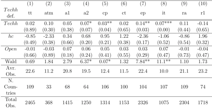
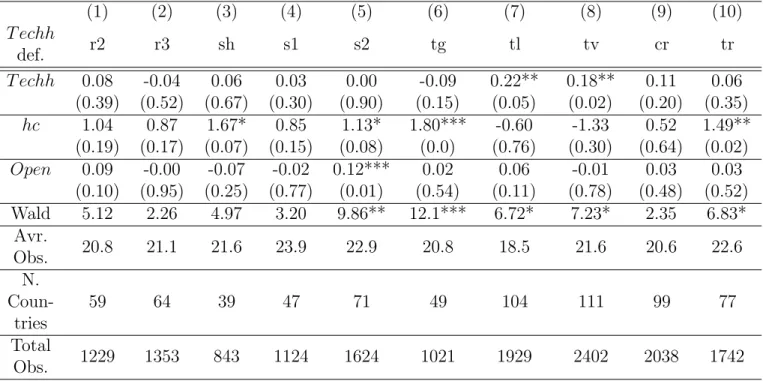
Tables 2 and 3 present the results. Results indicate positive and significant effects of avia-tion, cell phones, electric producavia-tion, internet, telephone and TV on income inequality. This broadly confirms the theoretical results according to which ICT and general purpose technolo-gies (such as aviation and electricity) adoption tend to increase inequality. Quantitatively, significant elasticities are between 0.03 (cellphones) to 0.22 (telephones), meaning, e.g., that a 1% increase in the use of telephones will imply an increase in inequality of 0.22%, for a given level of human capital. Interestingly the introduction of skill-complementary technologies in the regressions implies that a direct effect of human capital almost disappears, with only four exceptions, columns (3), (5), (6), and (10) in Table 3.

3_{For complete arguments toward reconsideration of traditional econometric methods to study moderate-T}

(8)

Table 2: Inequality and Technologies: Part I (1) (2) (3) (4) (5) (6) (7) (8) (9) (10) T echh def. tt atm a1 a2 cp ct ep it ra r1 T echh 0.02 0.10 0.05 0.07* 0.03** 0.02 0.14** 0.07*** 0.11 -0.14 (0.89) (0.30) (0.38) (0.07) (0.04) (0.65) (0.03) (0.00) (0.44) (0.65) hc -0.85 -2.33 0.34 0.68 0.95 1.22 -2.36 -1.06 -0.86 1.96 (0.49) (0.38) (0.66) (0.20) (0.21) (0.38) (0.17) (0.52) (0.54) (0.32) Open -0.01 -0.03 0.07 0.06 0.05 0.03 0.03 0.07 -0.01 -0.04 (0.66) (0.89) (0.18) (0.24) (0.41) (0.55) (0.29) (0.47) (0.73) (0.47) Wald 0.69 1.84 2.79 6.37* 0.07* 1.32 7.84** 11.1** 1.10 1.73 Avr. Obs. 22.6 11.2 20.8 19.5 12.4 11.5 22.4 10.0 21.1 23.2 N. Coun-tries 109 33 68 64 106 100 104 107 109 74 Total Obs. 2465 368 1415 1250 1314 1153 2326 1075 2304 1718

Note: Dependent Variables natural logarithm of the Gini coefficient. Definitions: tt tractors; atm ATM machines; a1 aviation passengers; a2 -aviation cargo; cp - cellphones; ct-computers; ep- electricity production; ra- radios; r1 - length of rail lines. A constant is included in regressions but omitted from the table. Values in parentheses are p-values. P-values of coefficients are based on robust standard errors. Level of significance: *** for p-value<0.01; **for p-value<0.05;* for p-value<0.1. Lists of countries included in individual regressions are available upon request.

(9)

Table 3: Inequality and Technologies: Part II (1) (2) (3) (4) (5) (6) (7) (8) (9) (10) T echh def. r2 r3 sh s1 s2 tg tl tv cr tr T echh 0.08 -0.04 0.06 0.03 0.00 -0.09 0.22** 0.18** 0.11 0.06 (0.39) (0.52) (0.67) (0.30) (0.90) (0.15) (0.05) (0.02) (0.20) (0.35) hc 1.04 0.87 1.67* 0.85 1.13* 1.80*** -0.60 -1.33 0.52 1.49** (0.19) (0.17) (0.07) (0.15) (0.08) (0.0) (0.76) (0.30) (0.64) (0.02) Open 0.09 -0.00 -0.07 -0.02 0.12*** 0.02 0.06 -0.01 0.03 0.03 (0.10) (0.95) (0.25) (0.77) (0.01) (0.54) (0.11) (0.78) (0.48) (0.52) Wald 5.12 2.26 4.97 3.20 9.86** 12.1*** 6.72* 7.23* 2.35 6.83* Avr. Obs. 20.8 21.1 21.6 23.9 22.9 20.8 18.5 21.6 20.6 22.6 N. Coun-tries 59 64 39 47 71 49 104 111 99 77 Total Obs. 1229 1353 843 1124 1624 1021 1929 2402 2038 1742

Note: Dependent Variables natural logarithm of the Gini coefficient. Definitions: r2 - railway passengers; r3 - railway cargo; sh - ships; s1 - steel in blast oxygen furnaces; s2 - steel in electric arc furnaces; tg - telegrams; tl- telephones; tv- televisions; cr- passenger vehicles; tr - commercial vehicles. A constant is included in regressions but omitted from the table. Values in parentheses are p-values. P-values of coefficients are based on robust standard errors. Level of significance: *** for p-value<0.01; **for p-value<0.05;* for p-value<0.1. Lists of countries included in individual regressions are available upon request.

(10)

4.2 Influence of Technology Types

In order to summarize results we built a taxonomy of four technology types, as described above. We now present the results for the influence of those technology types on inequality. This also allows us to analyze the conditional effect of each technology type on inequality, which enables answering the question if inequality rises due to e.g. ICT for the same adoption

of other technology types. Thus, T echhjit now assumes one of the four types: modern ICT,

older ICT, production, or transportation.

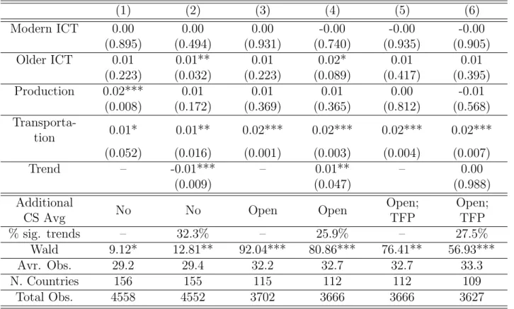
We continue to employ Pesaran (2006) common correlated effects estimator but we also im-plement slightly modified common correlated effects estimators suggested in recent literature. We include in the regressions one or more additional covariates in the form of cross-section averages, which helps to identify the unobserved common factors (in the spirit of Pesaran et al., 2013 and following what Eberhardt and Presbitero, 2014 did in an empirical imple-mentation). To this end, we consider openness as a cross-section average, seeking to identify the unobserved common factors as linked with globalization and global integration (e.g. the entrance of China in global markets affecting all the countries). In some of the regressions, together with openness we also considered averaged TFP as an additional control. This is to identify the unobserved common factors also with productivity spillovers around the world. Given that we now have available several more time-series observations per country, we present specifications with country trends, as well as information on their significance across countries. Table 4 presents these results.

Results indicate a highly significant effect of transportation technologies adoption on the increase of inequality, conditional on the adoption of other technology types. Thus, it seems that countries that adopted more transportation technologies than other technologies have also faced, due to that, an increase in inequality. This is a somewhat unexpected result, as theory has focused more on information and communication technologies as a source of in-equality. Countries that adopted more transportation technology may be highly integrated in world trade and thus be highly competitive. This can influence the wages of the most adaptable workers and thus increase inequality. In fact, transportation technologies are gen-eral purpose technologies in the sense that they are applied to the economy as a whole, with important effects on sectoral and countries integration. Results also reveal positive effects of older ICT technologies (specifications (2) and (4)) and of production technologies (specifica-tion (1)). Curiously, modern ICT has a non-significant effect on inequality, condi(specifica-tional on other technology-types adoption. Quantitatively, the effects mean that a 1 standard-deviation increase in a skill-complementary transportation technology (s.e.=3.37) would increase inequal-ity by 3.37% to 6.74%. If the 1 standard-deviation rise occurs in the older ICT technologies (when significant), for a s.e. equal to 1.90, the implied rise in inequality will amount to a value between 1.90% and 3.80%. Finally, If the 1 standard-deviation rise occurs in the production technologies (when significant), for a s.e. equal to 1.66, the implied rise in inequality will amount to 3.32%.

It is interesting to evaluate if these results differ from rich countries to poor countries, even before we analyze effects by individual country. Several features that could influence the relationship between skill-complementary technologies and inequality are quite different between rich and poor countries. The level of education, the composition between general and vocational education, and the proximity to the technology leader are only some of them.

(11)

Table 4: Inequality and Technology-types (1) (2) (3) (4) (5) (6) Modern ICT 0.00 0.00 0.00 -0.00 -0.00 -0.00 (0.895) (0.494) (0.931) (0.740) (0.935) (0.905) Older ICT 0.01 0.01** 0.01 0.02* 0.01 0.01 (0.223) (0.032) (0.223) (0.089) (0.417) (0.395) Production 0.02*** 0.01 0.01 0.01 0.00 -0.01 (0.008) (0.172) (0.369) (0.365) (0.812) (0.568) Transporta-tion 0.01* 0.01** 0.02*** 0.02*** 0.02*** 0.02*** (0.052) (0.016) (0.001) (0.003) (0.004) (0.007) Trend – -0.01*** – 0.01** – 0.00 (0.009) (0.047) (0.988) Additional

CS Avg No No Open Open

Open; TFP Open; TFP % sig. trends – 32.3% – 25.9% – 27.5% Wald 9.12* 12.81** 92.04*** 80.86*** 76.41** 56.93*** Avr. Obs. 29.2 29.4 32.2 32.7 32.7 33.3 N. Countries 156 155 115 112 112 109 Total Obs. 4558 4552 3702 3666 3666 3627

Note: Dependent Variables natural logarithm of the Gini coefficient. A constant is included in regressions but omitted from the Table. Values between parentheses are p-values. P-values on coefficients are based on robust standard errors. Level of significance: *** for p-value <0.01; **for p-value<0.05;* for p-value<0.1. Additional CS Avg means the additional variables added as controls as cross-section averages. % sig. trends is the percentage of country-trends that are statistically significant at the 5% level. Lists of countries included in individual regressions are available upon request.

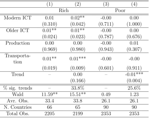
We next present results in which we divided the sample by the average GDP per capita, after averaging GDP per capita inside each country. Results shown in Table 5 highlight that the robust effects described above are all due to very strong positive effects of the technology types adoption that occur in rich countries. In fact, in rich countries, both transportation technologies and old ICT adoption are associated with high inequality and also modern ICT causes inequality when a trend is considered (column (2)), confirming the theory result and existing evidence relating ICT to inequality (e.g. in Jaumotte et al. (2013)). In the sample of the poorest countries, it is not possible to identify any significant effect of skill-complementary technology on inequality.

4.3 Robustness

We have also tested our results against differences in the implemented estimator and in a restricted sample. The alternative estimator was developed by Eberhardt and Teal (2010), seeking to identify the common unobserved effects with a single common factor designed to estimate a residual such as TFP. The restricted sample is one with higher populated time-series in which we restricted the sample to the countries that had more than 15 time-time-series

(12)

Table 5: Inequality and Technology-types: Rich and Poor Countries (1) (2) (3) (4) Rich Poor Modern ICT 0.01 0.02** -0.00 0.00 (0.310) (0.042) (0.711) (1.000) Older ICT 0.01** 0.01** -0.00 0.00 (0.024) (0.023) (0.787) (0.676) Production 0.00 0.00 -0.00 0.01 (0.969) (0.980) (0.943) (0.307) Transporta-tion 0.01** 0.01*** -0.00 -0.00 (0.019) (0.009) (0.601) (0.911) Trend – 0.00 – -0.01*** (0.166) (0.004) % sig. trends – 33.8% – 25.6% Wald 11.59** 15.51** 0.49 1.23 Avr. Obs. 33.4 33.8 26.1 26.1 N. Countries 66 65 90 90 Total Obs. 2205 2199 2353 2353

Note: Dependent Variables natural logarithm of the Gini coefficient. Values in parentheses are p-values. A constant is included in regressions but omitted from the table. P-values of coefficients are based on robust standard errors. Level of significance: *** for p-value <0.01; **for p-value<0.05;* for p-value<0.1. Additional CS Avg means the additional variables added as controls as cross-section averages. % sig. trends is the

(13)

observations for the dependent variable.

Generally, the robustness analysis presented in Table 6 confirms our previous results. Trans-portation technology increases inequality throughout all the considered specifications with sim-ilar quantitative effects as those obtained previously. Additionally older ICT also contributes to the rise in inequality in specifications in which a (statistically significant) trend is intro-duced in the regression. The specifications based on the Eberhardt and Teal (2010) estimator tend to increase the positive effect of modern ICT and in the specification with a (statistically significant) trend - column (4) - it also becomes highly significant. We have also divided the sample between rich and poor countries as we did before and use the Eberhardt and Teal (2010) estimator.4 _{Besides the significant effects obtained in the rich countries sample presented in}

Table 5, we have also obtained for the poor countries positive and highly significant (2.2% and 6.9% levels of significance respectively) coefficients for new and old ICT.

We performed an additional test on all results (which we do not show but are available upon request). Until now our measure of skill-complementary technology is a measure affected by scale, i.e., technological adoption is taken as total technological adoption, thus being influ-enced by the size of the country. This does not raise any particular problem de per si, since the inequality index is independent of the size of the country as well as human capital and open-ness. The conclusion is that some of those skill-complementary technology adoption affected by scale tend to influence inequality rises. Does an alternative per capita skill-complementary technology adoption measure which would be scale-independent have the same effect on in-equality? We re-ran all the regressions in the paper with these alternative measures (consisting of dividing the measure in (2) by the population in each year and country). Conclusions are as follows:

• Cellphone, internet, telephone, and TV adoption cause more inequality in specifications similar to those in Tables 2 and 3;

• Telegraph adoption contributes to decrease inequality in specifications similar to those in Tables 2 and 3;

• Transportation, production, and older ICT are still significant as determinants of (more) inequality in several regressions specified as in Table 4;

• Transportation technologies and modern ICT are still responsible for higher inequality in rich countries, as specified in Table 5;

• Production technologies and older ICT are significant determinants in the Pesaran (2006) specification, in specifications similar to those in Table 6;

• Older ICT is the only significant determinant of higher inequality in the Eberhardt and Teal (2010) specification, in a specification similar to that in Table 6.

Thus, surprisingly, despite a complete re-definition of the relevant measures for skill-complementary technologies adoption, removing the scale dimension of variables, results are quite consistent to those obtained when using the scale affected measure of skill-complementary technology adoption. The main difference is that some of the significant effects of the individual

(14)

technologies disappeared but other ICT effects are maintained. When technology-types mea-sures are considered, production technologies become relatively more important in explaining higher levels of inequality than before, maintaining the relative importance of transportation, old, and modern ICT.

Finally, we wish to discuss a possible alternative to construct the measures of technology types. Alternatively to what has been done, we could have restricted the technology types measures on observations for which all the components presented non-missing values. Due to the fact that this sample is highly unbalanced, doing so would imply very few observations for the technology types variables which would imply that a regression with the four variables as regressors would simply not be possible. However, it would be possible to evaluate the (non-conditional) effect of each technology type to evaluate if, for example, it is crucially different from the conditional one. Interestingly, when testing individually the technology-types variables (restricted to non-missing observations in all the components), despite a huge drop in the number of observations (from nearly 4500 as in Table 6 to around 500), all the technology-types have highly significant and positive coefficients (at 1% level), with coefficients oscillating from nearly 0.06 for all technology-types except older ICT type, and 0.14 for older ICT type, highlighting also positive and significant effects for those restricted measures for technology-types.

4.4 Results by Country

This section reports the results by individual country. For this we consider the restricted sample with high populated time-series considered also in Table 6. This is done in order to maximize time-series availability within countries. Tables 7, 8, and 9 show the statistically significant results by country.

These results highlight the great heterogeneity of the effects of technology adoption on in-come inequality by country. Despite some globally non-significant signs, there might be a wide range of countries in which technological adoption tends to decrease or increase inequality. Additionally, despite the overall positive signs of the skill-complementary technological adop-tion coefficients, there might be some countries in which there is evidence that technological adoption decreases inequality.

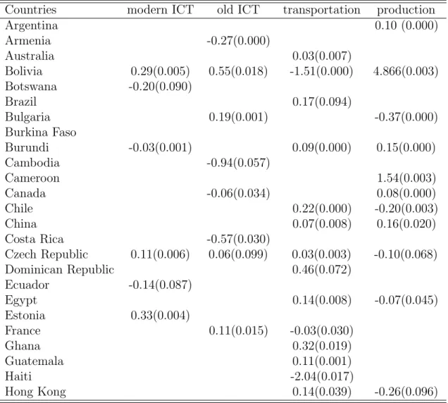
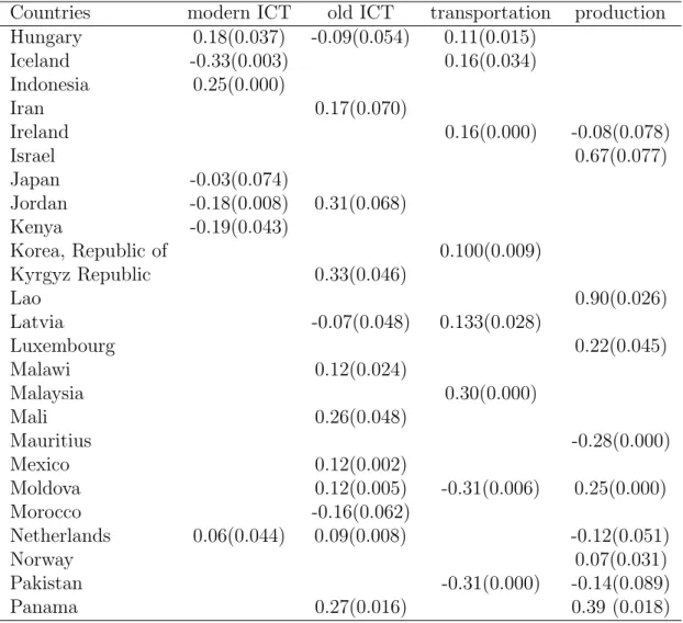
Of the 131 countries entering in regressions (see e.g. columns (3) to (6) in Table 6), there are 75 with significant coefficients in at least one technology-type. As expected, most of the countries present positive signs, i.e., technology adoption causes higher inequality. There are 11 countries in which modern ICT adoption tends to raise inequality and 8 in which this technology type tends to decrease inequality. Among the first group, we find countries such as Netherlands, Iceland, United Kingdom, Thailand and Indonesia. Among the second, we identify countries like Switzerland, Japan, Burundi and Equador. There are many more countries with significant coefficients associated with other technology types than to modern ICT (29 to old ICT and transportation type and 34 to production type). There are 22 countries in which old ICT adoption tends to raise inequality and 7 in which this technology type tends to decrease inequality. Among the first group, we find countries such as France, Netherlands, Singapore, Sweden, Iran, Panama, Mali, and Malawi, to give some examples. Among the second, we identify countries such as Canada, Latvia, Cambodia and Costa Rica. There are 24 countries in which transportation technology-type adoption tends to raise inequality and

(15)

Table 6: Inequality and Technology-types: Robustness Analysis (1) (2) (3) (4) (5) (6) Estimator Eberhardt and Teal (2010) Eberhardt and Teal (2010) Eberhardt and Teal (2010) Eberhardt and Teal (2010) Pesaran (2006) Pesaran (2006)

Sample Total Highly Populated Time-Series (≥ 15)

Modern ICT 0.00 0.00 0.00 0.01** -0.00 0.00 (0.571) (0.126) (0.469) (0.050) (0.801) (0.881) Older ICT 0.00 0.01*** 0.01 0.01*** 0.01 0.02** (0.450) (0.005) (0.296) (0.004) (0.160) (0.026) Production -0.00 -0.00 -0.01 0.00 0.02* 0.01 (0.262) (0.800) (0.135) (0.968) (0.092) (0.273) Transporta-tion 0.01* 0.01** 0.01** 0.01** 0.01* 0.01** (0.082) (0.039) (0.039) (0.023) (0.072) (0.037) Trend – 0.00** – 0.00*** – -0.00* (0.021) (0.009) (0.099) % sig. trends – 42.4% – 44.3% – 35.1% Wald 5.17 14.48*** 8.13* 17.39*** 8.12* 10.52** Avr. Obs. 29.4 30.0 32.8 32.8 32.8 32.8 N. Countries 155 151 131 131 131 131 Total Obs. 4552 4524 4301 4301 4301 4301

Note: Dependent Variables natural logarithm of the Gini coefficient. A constant is included in regressions but omitted from the table. Values in parentheses are p-values. P-values of coefficients are based on robust standard errors. Level of significance: *** for p-value <0.01; **for p-value<0.05;* for p-value<0.1. Additional CS Avg means the additional variables added as controls as cross-section averages. % sig. trends is the percentage of country-trends that are statistically significant at the 5% level.

(16)

Table 7: Countries statistically significant - Part 1

Countries modern ICT old ICT transportation production

Argentina 0.10 (0.000) Armenia -0.27(0.000) Australia 0.03(0.007) Bolivia 0.29(0.005) 0.55(0.018) -1.51(0.000) 4.866(0.003) Botswana -0.20(0.090) Brazil 0.17(0.094) Bulgaria 0.19(0.001) -0.37(0.000) Burkina Faso Burundi -0.03(0.001) 0.09(0.000) 0.15(0.000) Cambodia -0.94(0.057) Cameroon 1.54(0.003) Canada -0.06(0.034) 0.08(0.000) Chile 0.22(0.000) -0.20(0.003) China 0.07(0.008) 0.16(0.020) Costa Rica -0.57(0.030) Czech Republic 0.11(0.006) 0.06(0.099) 0.03(0.003) -0.10(0.068) Dominican Republic 0.46(0.072) Ecuador -0.14(0.087) Egypt 0.14(0.008) -0.07(0.045) Estonia 0.33(0.004) France 0.11(0.015) -0.03(0.030) Ghana 0.32(0.019) Guatemala 0.11(0.001) Haiti -2.04(0.017) Hong Kong 0.14(0.039) -0.26(0.096)

6 in which this technology type tends to decrease inequality. Among the first group, we find countries such as Australia, Iceland, Ireland, Burundi, China, Tanzania, and Thailand. The second group comprises Bolivia, France, Haiti, Moldova, Pakistan, and Ukraine. Despite the generally non-significant coefficient for the production-type technology adoption (see Tables 4 and 6), this is the technology-type with the highest number of significant coefficients per country (34). However, the number of negatively significant coefficients (16) is relatively close to the number of positively significant coefficients (18). Countries with a significantly positive sign for the production technology-type coefficient are, e.g., Argentina, Bolivia, Israel, Poland, and Spain. Countries with a significantly negative sign for the production technology-type coefficient are, e.g., Bulgaria, Chile, Hong-Kong, Pakistan, and Portugal. This means that despite the fact that a positive effect of some types of technology adoption in raising inequality was obtained for the panel database, mainly for the rich countries (see Table 5), it is undoubted that we can identify both rich and poor countries with significantly positive signs and with significantly negative signs.

(17)

Table 8: Countries statistically significant - Part 2

Hungary 0.18(0.037) -0.09(0.054) 0.11(0.015) Iceland -0.33(0.003) 0.16(0.034) Indonesia 0.25(0.000) Iran 0.17(0.070) Ireland 0.16(0.000) -0.08(0.078) Israel 0.67(0.077) Japan -0.03(0.074) Jordan -0.18(0.008) 0.31(0.068) Kenya -0.19(0.043) Korea, Republic of 0.100(0.009) Kyrgyz Republic 0.33(0.046) Lao 0.90(0.026) Latvia -0.07(0.048) 0.133(0.028) Luxembourg 0.22(0.045) Malawi 0.12(0.024) Malaysia 0.30(0.000) Mali 0.26(0.048) Mauritius -0.28(0.000) Mexico 0.12(0.002) Moldova 0.12(0.005) -0.31(0.006) 0.25(0.000) Morocco -0.16(0.062) Netherlands 0.06(0.044) 0.09(0.008) -0.12(0.051) Norway 0.07(0.031) Pakistan -0.31(0.000) -0.14(0.089) Panama 0.27(0.016) 0.39 (0.018)

5 Conclusion

Quantitative assessments of the determinants of inequality are scarce. So are the quantita-tive evaluations of the theories that assume that skills are complementary to technologies and jointly determine the evolution of inequality. In this work we seek to contribute to enrich that literature. To this end, we use very recent data on the Gini index, available for a wide range of countries and years and relate it with measures of skill-complementary technological adoption of 20 different technologies. First, we analyze each skill-complementary technology and evaluate its effect on inequality. We discovered that several skill-complementary technolo-gies contribute to the inequality rise and none contribute to the inequality drop. Adoption of technologies such as aviation, cell phones, electricity production, internet, telephone, and TV, contribute to increase inequality. Then, we construct four different measures of technology-types allowing us to evaluate the conditional contribution of each type to the evolution of inequality. We found strong evidence that older ICT and transport technologies (and less fre-quently modern ICT) tend to increase inequality. Thus, earlier emphasis in the literature on the effect of ICT in raising inequality is relatively shaken by our results, as modern ICT

(18)

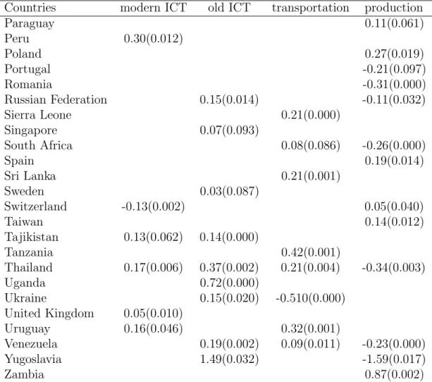
adop-Table 9: Countries statistically significant - Part 3

Paraguay 0.11(0.061) Peru 0.30(0.012) Poland 0.27(0.019) Portugal -0.21(0.097) Romania -0.31(0.000) Russian Federation 0.15(0.014) -0.11(0.032) Sierra Leone 0.21(0.000) Singapore 0.07(0.093) South Africa 0.08(0.086) -0.26(0.000) Spain 0.19(0.014) Sri Lanka 0.21(0.001) Sweden 0.03(0.087) Switzerland -0.13(0.002) 0.05(0.040) Taiwan 0.14(0.012) Tajikistan 0.13(0.062) 0.14(0.000) Tanzania 0.42(0.001) Thailand 0.17(0.006) 0.37(0.002) 0.21(0.004) -0.34(0.003) Uganda 0.72(0.000) Ukraine 0.15(0.020) -0.510(0.000) United Kingdom 0.05(0.010) Uruguay 0.16(0.046) 0.32(0.001) Venezuela 0.19(0.002) 0.09(0.011) -0.23(0.000) Yugoslavia 1.49(0.032) -1.59(0.017) Zambia 0.87(0.002)

tion is definitively not the most significant type of technology adoption in raising inequality. We also discovered that results are much stronger in rich countries than in poor. The use of heterogenous panel estimators allowed us to highlight the diversity of results among countries. Nevertheless, an overwhelming number of countries present an influence of increased skill-complementary technological adoption (mainly in older ICT and transportation technologies) on the increase of inequality.

Our results are robust to a series of modifications in specification, estimator, samples, and to the skill-complementary technological adoption measure.

These results may have policy implications for the design of incentives for adopting tech-nologies, especially for rich and well human-capital-endowed countries, in which the effect in the rise of inequality may be quite significant.

(19)

References

[1] Acemoglu, D. (2002a). Technical change, inequality and the labor market. Journal of Economic Literature, 40:7–72.

[2] Acemoglu, D. (2002b). Directed technical change. Review of Economic Studies, 69:781–810. [3] Acemoglu, D. (2003). Technology and Inequality. NBER Reporter.

[4] Aghion, P., Howitt, P., and Violante, G. (2002). General purpose technology and wage inequality. Journal of Economic Growth, 7(4):315–345.

[5] Barro, R. J. (2000). Inequality and Growth in a Panel of Countries. Journal of Economic Growth, 5(1):5–32.

[6] Caselli, F. (1999). Technological revolutions. American Economic Review, 89:78–102. [7] Comin, D. and Hobijn, B. (2009). The CHAT Dataset. NBER Working Papers 15319,

National Bureau of Economic Research, Inc.

[8] Comin, D., Rossi-Hansberg, E., and Dmitriev, M. (2013). The Spatial Diffusion of Tech-nology.

[9] Deininger, K. and Squire, L. (1996). New Data Set Measuring Income Inequality. World Bank Economic Review, 10:565–591.

[10] Ding, S., Meriluoto, L., Reed, W. R., Tao, D., and Wu, H. (2011). The impact of agri-cultural technology adoption on income inequality in rural China: Evidence from southern Yunnan Province. China Economic Review, 22(3):344–356.

[11] Eberhardt, M. and Presbitero, A. (2014). This Time They Are Different: Heterogeneity and Nonlinearity in the Relationship Between Debt and Growth. version 13th February 2014.

[12] Eberhardt, M. and Teal, F. (2011). Econometrics for Grumblers: a New Look At the Literature on Cross-Country Growth Empirics. Journal of Economic Surveys, 25(1):109– 155.

[13] Galor, O. and Moav, O. (2000). Ability biased technological transition, wage inequality within and across groups, and economic growth. Quarterly Journal of Economics, 115:469– 497.

[14] Galor, O. and Tsiddon, D. (1997). Technological progress, mobility, and economic growth. American Economic Review, 87:362–382.

[15] Greenwood, J. and Yorukoglu, M. (1997). 1974. Carnegie-Rochester Conference Series on Public Policy 46, pages 49–96.

[16] Hornstein, A., Krusell, P., and Violante, G. L. (2005). Chapter 20 The Effects of Technical Change on Labor Market Inequalities. Handbook of Economic Growth, 1:1275–1370.

(20)

[17] Jaumotte, F., Lall, S., and Papageorgiou, C. (2013). Rising Income Inequality: Technol-ogy, or Trade and Financial Globalization? IMF Economic Review, 61(2):271–309.

[18] Pesaran, M. H. (2006). Estimation and Inference in Large Heterogeneous Panels with a Multifactor Error Structure. Econometrica, 74(4):967–1012.

[19] Pesaran, M. H., Smith, V., and Yamagata, T. (2013). Panel Unit Root Tests in the Presence of a Multifactor Error Structure. Journal of Econometrics, 175(2):94–115.

[20] Pesaran, M. H. and Tosetti, E. (2011). Large Panels with Common Factors and Spatial Correlations. Journal of Econometrics, 161(2):182–202.

[21] Ratts, J. and Stokke, H. (2013). Regional Convergence of Income and Education: Inves-tigation of Distribution Dynamics. Urban Studies, Published online before print August 19, 2013, doi: 10.1177/0042098013498625.

[22] Solt, F. (2009). Standardizing the World Income Inequality Database. Social Science Quarterly, 90(2):231–242.

(21)

A

Appendix

A.1 List of Technologies and Abbreviations

• wheel and crawler tractors (excluding garden tractors); definition in the source: tractor; abbreviation: tt

• electromechanical devices that permit authorized users, typically using machine read-able plastic cards, to withdraw cash from their accounts and/or access other services; definition in the source: atm; abbreviation: atm

• Civil aviation passenger-KM traveled on scheduled services by companies registered in the country concerned. Not a measure of travel through a country airports; definition in the source: aviationpkm; abbreviation: a1

• Civil aviation ton-KM of cargo carried on scheduled services by companies registered in the country concerned. Not a measure of travel through a country’s airports; definition in the source: aviationtkm; abbreviation: a2

• Number of users of portable cell phones; definition in the source: cell phone; abbreviation: cp

• Number of self-contained computers designed for use by one person; definition in the source: computer; abbreviation: ct

• Gross output of electric energy (inclusive of electricity consumed in power stations) in KwHr; definition in the source: elecprod; abbreviation: ep

• access to the worldwide network; definition in the source: internetuser; abbreviation: it • Number of Radios; definition in the source: radio; abbreviation: ra

• Geographical/route lengths of line open at the end of the year. Narrow gauge lines generally included, but mountain railways, purely industrial lines not open to the public, and urban systems generally excluded; definition in the source: railline; abbreviation: r1 • Passenger journeys by railway in passenger-KM. Free passengers typically excluded but may be included for some countries; definition in the source: railpkm; abbreviation: r2 • freight carried on railways (excluding livestock and passenger baggage). Freight for

ser-vicing of railroads is typically excluded but may be included for some countries; definition in the source: railtkm; abbreviation: r3

• steamships (above a minimum weight) in use at midyear; definition in the source: shipton-steammotor; abbreviation: sh

• Crude steel production (in metric tons) in blast oxygen furnaces (a process that replaced Bessemer and OHF processes); definition in the source: steel-bof; abbreviation: s1

(22)

• Crude steel production (in metric tons) in electric arc furnaces (a process that com-plemented and improved upon Bessemer and OHF processes); definition in the source: steel-eaf; abbreviation: s2

• Telegrams; definition in the source: telegram; abbreviation: tg

• mainline telephone lines connecting a customer’s equipment to the public switched tele-phone network as of year end; definition in the source: teletele-phone; abreviation: tl

• television sets in use; definition in the source: tv; abbreviation: tv

• passenger cars (excluding tractors and similar vehicles) in use. Numbers typically derived from registration and licensing records, meaning that vehicles out of use may occasionally be included.; definition in the source: vehicle-car; abbreviation: cr

• commercial vehicles, typically including buses and taxis (excluding tractors and similar vehicles), in use. Numbers typically derived from registration and licensing records, meaning that vehicles out of use may occasionally be included; definition in the source: vehicle-com; abbreviation: tr