Real-time Simulation of
a Mobile Machine
Dissertação para obtenção do Grau de Mestre em Engenharia Mecânica
Orientador: Professor Doutor Alberto Martinho,
Professor Auxiliar, FCT-UNL
Co-orientador: Professor Doutor Aki Mikkola,
Professor, LUT
Júri:
Presidente: Prof. Doutor António José Freire Mourão Arguente: Prof. Doutor Tiago Alexandre Narciso da Silva Vogal: Prof. Doutor Alberto José Antunes Marques
Martinho Outubro, 2019
iii Real-time simulation of a mobile machine
Copyright © Tomás Correia Coimbra Mano, Faculdade de Ciências e Tecnologia, Universidade Nova de Lisboa.
A Faculdade de Ciências e Tecnologia e a Universidade Nova de Lisboa têm o direito, perpétuo e sem limites geográficos, de arquivar e publicar esta dissertação através de exemplares impressos reproduzidos em papel ou de forma digital, ou por qualquer outro meio conhecido ou que venha a ser inventado, e de a divulgar através de repositórios científicos e de admitir a sua cópia e distribuição com objetivos educacionais ou de investigação, não comerciais, desde que seja dado crédito ao autor e editor.
v
Acknowledgements
This work was made possible due to the efforts of some people I would like to acknowledge.First, to all the people I got to know at LUT, for the help given, for the possibility to develop this thesis and for the chance to learn more about real-time simulation. To professor Aki, who made it possible for me to develop my work abroad, for all the help given related with the work and with life in Finland. To Qasim and Nima, for making it easier to understand the software and to perform the necessary tests.
To all my friends, who were always a phone call away, to answer any questions and for the support given throughout these past months when this work seemed to be impossible to complete. For my friends, developing their works at the same time as me, supporting is key, and thank you for all the love.
To my supervisor in Portugal, professor Alberto Martinho, for all the help given, for going along in this journey with my, always available to answer my questions.
Finally, to my family, my mother and father, my grandparents, and all the others involved in making my time in Finland possible, and to my brothers, in spite of not being there with me, were always there for me.
vii
Abstract
Real-time simulation is becoming a useful tool to improve products and efficiency in product development. Being able to perform real-time dynamic analysis on a virtual prototype helps engineers improve products faster, with a reduction in the associated costs. The possibility to analyse complex systems using powerful software that enable the creation of simpler models which can accurately represent these systems, allows the use of tools to perform numerical integrations and dynamic analysis in a faster, simpler, and easier way.With the growth of real-time simulation, gamified simulations are also improving and becoming a tool for product development. The goal of turning mechanical simulations into game-like environments is to encourage users to test products, providing important information to manufacturers, and making the product development to be more customer oriented.
This thesis explores two topics. The first part consists of developing a dynamic analysis of a forklift, using the existing theoretical definitions and implementing them using Mevea software. The system’s behaviour will be studied by imposing different conditions and comparing the outcomes (differences in the behaviour of the machine). The second part aims at using the developed model to create a gamified simulation. The simulation should become user-friendly with a goal and tasks to be performed, encouraging users to test the created model. All this is achieved by adding different game elements. Ultimately, the goal of the simulation is to obtain information from the users about their experience, to improve the model and, consequently, the forklift, to suit the needs of the users.
The goal of this thesis is to understand the benefits of real-time dynamic analysis, as well as to evaluate gamified simulations as a tool for engineers to get important information during product development.
ix
Resumo
A simulação em tempo real tem vindo a tornar-se uma ferramenta útil na melhoria de produtos e no aumento da eficiência na fase de desenvolvimento de um produto. A possibilidade de realizar uma análise dinâmica em tempo real a um protótipo virtual permite aos engenheiros melhorar os produtos mais rapidamente, e com uma redução de custos associada. A possibilidade de analisar sistemas complexos utilizando software que permite a criação de modelos simplificados que conseguem representar o sistema de maneira eficaz, permite o uso de ferramentas para realizar as integrações numéricas e a análise dinâmica de maneira mais eficiente, simples e rápida.Com o crescimento da simulação em tempo real, as simulações estilo “jogo” também têm vindo a melhor, tendo se tornado uma ferramenta útil para o desenvolvimento de produtos. O objetivo de transformar as simulações em ambientes semelhantes a jogos é encorajar os utilizadores a testarem os produtos e a fornecer feedback aos fabricantes, permitindo que o produto seja desenvolvido tendo em conta as necessidades dos utilizadores.
Esta dissertação explora dois tópicos. A primeira parte consiste em realizar uma análise dinâmica a uma empilhadora, recorrendo a formulações teóricas existentes, e implementando-as com recurso ao software Mevea. O comportamento da empilhadora deve ser estudado, considerando diferentes casos e comparando os resultados (alterações no comportamento da máquina). A segunda parte consiste em utilizar o modelo desenvolvido na criação de uma simulação estilo “jogo”. Esta simulação deve ser centrada no utilizador e deve conter um objetivo claro e as instruções necessárias, encorajando os utilizadores a testarem o modelo. Tudo isto é feito através da introdução de elementos de jogo. Em última análise deverá ser possível avaliar as experiências dos utilizadores e utilizar a informação proveniente das simulações para melhorar a empilhadora.
Este trabalho tem como objetivo a perceção dos benefícios da análise dinâmica em tempo real, bem como avaliar como as simulações estilo “jogo” podem fornecer informação importante aos projetistas.
Palavras chave: simulação em tempo real, Análise dinâmica, simulação estilo “jogo”, elementos de jogo, utilizadores
xi
Table of contents
Acknowledgements ... v Abstract ... vii Resumo ... ix Table of contents ... xiList of Figures ... xiii
List of tables ... xvii
List of Symbols and Abbreviations ... xix
1 Introduction ... 1 1.1 Context ... 1 1.2 Objectives ... 3 1.3 Research Methodology ... 4 1.4 Thesis Structure ... 5 2 Methodology ... 7 2.1 Multibody Systems ... 7
2.2 Description of rigid bodies ... 8
2.3 Kinematic Analysis ... 10
2.4 Dynamic Analysis ... 12
2.5 Numerical Integration ... 19
2.6 Collision and contact modelling ... 24
2.7 Hydraulic circuit ... 26
2.8 Computer-aided simulation ... 31
3 Gamification ... 35
3.1 Game Elements ... 36
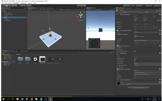
3.2 Unity software ... 38
3.3 Mevea and Unity interface ... 38
xii 3.5 Related work ... 40 4 Case Study ... 47 4.1 Forklift... 47 4.2 Simulation model ... 50 4.3 Environment ... 58 4.4 Gamification ... 60 5 Results ... 71 5.1 Dynamic analysis ... 71
5.2 Simulation and gamification ... 76
6 Discussion ... 79
6.1 Dynamic analysis ... 79
6.2 Hydraulic analysis ... 81
6.3 Simulation and Gamification ... 82
6.4 Other considerations ... 86
7 Conclusion ... 89
Bibliographic References ... 91
Appendix ... 95
xiii
List of Figures
Figure 1.1 Advantages of modelling and simulation ... 2
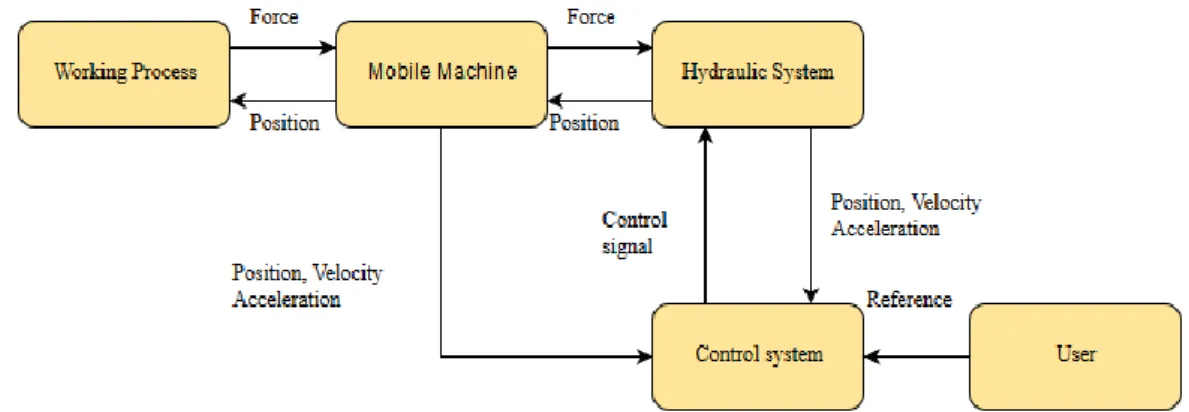
Figure 1.2 Systems needed to build a simulation for a mobile machine ... 4
Figure 2.1 Multibody System ... 7
Figure 2.2 Global vs. Local coordinate system ... 8
Figure 2.3 Tree structure of a multibody system... 17
Figure 2.4 Arbitrary pair of bodies Bj-1 and B ... 18
Figure 2.5 Numerical integration in dynamic analysis ... 21
Figure 2.6 Euler's method ... 22
Figure 2.7 Rung-Kutta second order method ... 22
Figure 2.8 Fourth-order Runge-Kutta method ... 23
Figure 2.9 Simulation model vs. collision model ... 24
Figure 2.10 Collision detection between two bodies ... 25
Figure 2.11 Contact between two bodies ... 25
Figure 2.12 Unit sized hydraulic volume ... 26
Figure 2.13 Laminar flow and turbulent flow ... 27
Figure 2.14 Hydraulic system with two volumes ... 28
Figure 2.15 Hydraulic volume ... 29
Figure 2.16 Hydraulic cylinder ... 31
Figure 2.17 Chronological principle of real-time simulation ... 32
Figure 2.18 Mevea modeller and Mevea solver ... 34
Figure 3.1 Unity interface ... 38
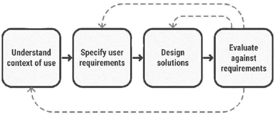
Figure 3.2 UX user-centred ... 39
Figure 3.3 Multibody dynamics simulation in product development ... 41
Figure 3.4 Three possible outputs expected for the arrangement of loads ... 42
Figure 3.5 Model for the robotic arm ... 42
xiv
Figure 3.7 Tree truck harvester ... 44
Figure 3.8 Excavator model ... 45
Figure 3.9 Simulation interface ... 45
Figure 4.1 Forklift presented in the catalogue ... 47
Figure 4.2 Forklift model ... 48
Figure 4.3 Joint schematics ... 49
Figure 4.4 Front wheels schematics ... 49
Figure 4.5 Back wheels schematics ... 50
Figure 4.6 Forklift model ... 51
Figure 4.7 Main Body ... 52
Figure 4.8 Chain pulley system ... 52
Figure 4.9 a) First stage mast b) Second stage mast c) Load carrier ... 53
Figure 4.10 a) Rear axle b) pulley holder ... 53
Figure 4.11 a) tyre b) pulley ... 53
Figure 4.13 a) Lift cylinder b) Lift piston c) Tilt cylinder d) Tilt piston ... 54
Figure 4.14 Simplified hydraulic circuit. 1- Pulley lift; 2- First stage mast right lift; 3- First stage mast left lift; 4- Mast right tilt; 5- Mast left tilt; 6- DV22 Lift; 7- Counter-balance lift valve; 8- DV43 tilt valve; 9- DV43 lift valve; 10 – Volume pump; 11 – Volume tank ... 57
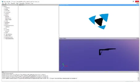
Figure 4.15 Simulation environment using Mevea ... 59
Figure 4.16 Simulation environment using Unity ... 59
Figure 4.17 Gamification the simulation process ... 60
Figure 4.18 User needs ... 61
Figure 4.19 Mevea simulation ... 63
Figure 4.20 Game-elements ... 64
Figure 4.21 On-screen information a) Goals b) Input information ... 65
Figure 4.22 Score system ... 65
Figure 4.23 On-game information a) Arrows showing the correct path b) Load dropping area . 66 Figure 4.24 Car elements ... 66
xv
Figure 4.25 Constraint elements a) Timer b) Containers for the collision system ... 67
Figure 4.26 Game chart ... 68
Figure 4.27 Inputs ... 69
Figure 5.1 Lifting system position analysis considering no load ... 72
Figure 5.2 Lifting system velocity analysis considering no load ... 72
Figure 5.3 Lifting system position analysis for a load = 2000Kg ... 72
Figure 5.4 Lifting system velocity analysis for a load = 2000Kg ... 73
Figure 5.5 Velocity analysis ... 73
Figure 5.6 Acceleration analysis ... 74
Figure 5.7 Hydraulic lifting components position analysis considering no load ... 75
Figure 5.8 Hydraulic lifting components velocity analysis considering no load ... 75
Figure 5.9 Hydraulic lifting components position analysis for a load = 2000 Kg ... 76
Figure 5.10 Hydraulic lifting components velocity analysis for a load = 2000 Kg ... 76
Figure 5.11 Loop time and step time comparison ... 77
xvii
List of tables
Table 3.1 Types of users ... 36
Table 4.1 Weight of the system ... 54
Table 4.2 Joint specifications ... 55
Table 4.3 Hydraulic components data ... 58
Table 6.1 Rosewater´s features ... 85
Table 8.1 Main body ... 95
Table 8.2 First Mast ... 95
Table 8.3 Second mast ... 95
Table 8.4 Load carrier ... 96
Table 8.5 Pulley holder ... 96
Table 8.6 Rear axle ... 96
xix
List of Symbols and Abbreviations
Initials and acronyms
DAE – Differential algebraic equations ODE – ordinary differential equations DOF’s – Degrees of Freedom
CAD – Computer Aided Design
CAM – Computer Aided Manufacturing CASE – Computer Aided Software Engineering
CAS – Computer Aided Simulation VR – Virtual Reality
Vectors/matrix
𝐪/𝐫𝐼𝑖 – Global position of a particle 𝐪̇/𝐫̇𝐼𝑖 – Velocity of a particle 𝐪̈/𝐫̈𝐼𝑖 – Acceleration
𝐑𝐼 – Global position of a body
𝐑̇𝐼 – Velocity of a body
𝐑̈𝐼 – Translational acceleration of a body
𝐮
̅𝐼𝑖 – Position a particle relatively to the local coordinate system
𝐀𝑖 – Coordinates transformation matrix
𝐀̇𝑖/𝐀𝜃,𝐴 – Derivative of rotation matrix
𝛚𝑖 – Angular velocity of a body
𝛚̇𝑖 – Angular acceleration of a body
∆𝐪 – displacement
𝛿𝐫𝐴 – Virtual displacement
𝛿𝐖𝐴 – Virtual work
𝐪̇∗ - Virtual velocity
𝝎∗ - Virtual angular velocity
M – Mass Matrix
𝐈𝑛 – Identity matrix of index n
𝐉𝟎 – Rotation inertia tensor
C – Quadratic velocity vector F –Force vector
Q – Generalized forces vector T - Torque 𝐖∗ - Virtual Power 𝛌 – Lagrange multipliers 𝚽𝐪/𝚽(𝐪, 𝑡) – Displacement constraints 𝚽̇(𝐪̇, 𝑡)/𝚽̇(𝐪, 𝐪̇ , 𝑡)– Velocity constraints 𝐂𝐪𝐂𝐪 – Jacobian matrix 𝐂𝐪 – Jacobian matrix 𝚽̇(𝐪̇, 𝑡) – velocity constraints 𝐑 – Velocity transformation matrix 𝐑̇ – Time derivative of 𝑅
𝐳̇ – Relative joint velocity 𝐳̈ – Relative joint acceleration 𝐳̇∗ - Independent velocities vector
𝐅𝐧 – Normal forces
𝐅𝐭 – Tangential forces
xx
𝐕𝑛 – Relative velocity of a collision
𝐧 – normal vector 𝐅𝛍 – Friction Force
Scalar values
𝜃𝑖 – Angle between the local coordinate and
the global coordinate systems 𝜃̇𝑖 – Angular velocity of a particle
𝜃̈𝑖 – Angular velocity of a particle
𝛚𝑖 – skew-symmetric matrix of 𝜔𝑖x – Displacement along the X axis
y – Displacement along the Y axis 𝑡𝑖 – Time at instant i
∆𝑡 – time step
𝑥̇∗ - Virtual velocity along the X axis
𝑦̇∗- virtual velocity along the Y axis
𝑚 - number of constraint equations 𝑛 – Number of dependent coordinates 𝑓 – Number of degrees of freedom 𝑂(ℎ𝑝+1) – local truncation error 𝑂(ℎ𝑝) – method’s order
𝜌 - Density B – Bulk modulus
𝐵𝑒 – Effective bulk modulus
𝑄𝑖 – Flow rate 𝑣 - Velocity 𝑘 – Spring coefficient 𝑠 – Damping coefficient 𝑉 - Volume 𝑑𝑉 – Volume change 𝑑𝑝 – Pressure change 𝑅𝑒 – Reynolds number 𝐷ℎ - Hydraulic diameter 𝜐 - Viscosity 𝑚̇ – mass flow rate 𝐶𝑣 – Flow rate constant
𝑋0 – Relative spool position
𝑈𝑟𝑒𝑓 – Reference voltage signal
𝜏 – Time constant
Note: All the vector and matrixes presented throughout this work are presented in normal bold characters while the scalar values are presented in italic without bold
1
1 Introduction
The first chapter starts by introducing the work that will be developed, the approach to the problem, the objectives proposed and how this thesis will be developed.
1.1
Context
Mechanical engineering is often associated with innovation. With industrial growth and development, productivity, efficiency, and competitiveness are now issues that engineers must face. It is necessary to improve how engineers work and how projects and products are developed and tested. It is necessary to work with the existing tools, but in a better way, to boost productivity levels. The processes need to be fully understood in order to increase the efficiency of the project and, consequently, of the product (Larsson, 2001).
Computational mechanics, and more specifically multibody system dynamics, is one of the available tools used for performing dynamic analysis of complex systems (where the system’s behaviour is analysed, having the time as a constraint). This area is responsible for dealing with the kinematics and the dynamics of systems, numerical methods, optimization, and control issues (Schiehlen, 2006).
Combining multiple areas in computational mechanics, like multibody dynamics and computer-aided design (CAD) makes it possible for engineers to work faster and in a more efficient way. The possibility to use a tool to build a trustworthy model (to represent a product) together with the possibility to test that model as a virtual prototype allows engineers to obtain a better and faster understanding of most of the problems that might exist when testing different solutions for a project. This way, virtual models become virtual prototypes that can represent the properties of a physical prototype accurately, and the analysis becomes faster and can commit fewer errors, compared with traditional methods.
In the industry field, the demand for better, safer, and more efficient solutions made engineers change the way they develop and test solutions. The possibility of a faster and more efficient analysis (using computational tools) with a model made engineers turn to real-time simulations. This type of simulation appears as a solution because it allows the model to be tested in real time, eliminating time-delay as a constraint.
2
Real-time simulation reduces the necessity of creating many physical prototypes, which most of the times are tested with the wrong parameters and have the wrong properties. Physical prototypes often need multiple versions to perform different tests, until the best version is achieved. A virtual prototype allows testing the different parameters and conditions without the need of creating numerous versions with different physical properties, eliminating the costs associated with the process and achieving the same outcome faster. It also allows for a better understanding of how the different systems interact, making it possible to make more efficient products. The three major benefits related to efficiency are reduced costs, accelerated schedule, and improved product quality (US Army, 2013).
Figure 1.1 shows the benefits of modelling and simulation when applied to product development. The major benefits regarding the project are testing, user-engagement, and safety.
Figure 1.1 Advantages of modelling and simulation, adapted from (US Army, 2013)
Mobile machines of every type are essential in modern industry. Every machine needs to keep improving the safety standards and its efficiency in order to satisfy the rules and safety parameters. The demand leads to the necessity of developing better ways to improve mobile machines, simplifying its controls and improving overall features.
To help developing better machines and better professionals, simulation models with real-time simulation applications are being developed. It becomes easier to evaluate the machine due to its complexity and to improve the design or functioning features.
3 Mechanical real-time simulation has one problem. It can become boring when testing the products. If the simulation lacks interaction with whoever tests it, it can lead to a loss of interest, producing average results and not representing a sucessful test. The best way to create a simulation that does not become boring is to keep improving the interaction features (game elements or motivational factors).
Because the simulations can be tested by users to get feedback and to improve the product in a more customer-oriented way, they should be appealing and keep users interested in them. If these simulations are boring, users might not feel interested in testing them, making the feedback available less trustful, delaying the improvement process. Engineers, to solve this problem, started introducing game elements to the simulations, making them more appealing but maintaining realism. The introduction of game elements in simulations allows better feedback from users, making the simulation more engaging, motivating users to perform any given tasks. This way, getting more and better information about the products, engineers can evaluate the products from the customer´s point of view, being able to think of products for a more customer-oriented production.
Since the beginning of the 21st century, articles about computationally aided simulation
and real-time simulation, as well as game-like environment simulation, have been published, proving the growing interest in this area.
1.2
Objectives
This thesis’ objective is to understand how multibody dynamic analysis works, to analyse a mobile machine (a forklift) and simulate it, using real-time simulation software, MEVEA, and add game elements to the simulation, using UNITY, in order to comprehend how different bodies interact with each other, and how gamification helps getting better and more accurate information about a product.
Some questions like the ones presented below should be answered at the end of this thesis:
▪ What are the benefits of real-time dynamic analysis?
▪ What game elements can be added so that the simulation is effective and
motivates users to complete tasks?
▪ How manufacturers can use the information obtained through game-like
simulations?
4
To help understand and answer these questions, this thesis includes a methodology section where the key concepts, as well as the theoretical definitions and related work are presented before addressing the forklift study case. After the results are presented and discussed, it should be possible to answer the questions presented.
1.3
Research Methodology
Figure 1.2 describes the existing relations involving all necessary systems to build a simulation that truly represents a mobile machine. The external forces acting in the system, as well as the internal forces, make the system behave in a certain way. Position, velocity, and acceleration are necessary parameters to describe this behaviour and to predict what actuators need to do. All this information can be passed to a control panel that enables the user to see and control the system.
Figure 1.2 Systems needed to build a simulation for a mobile machine, adapted from (Mikkola, Lecture1_m, 2018)
To understand how a complex system behaves, it is necessary to comprehend how the different bodies behave individually and as a whole. It is also necessary to understand what joints can be used and what constraints (and consequently the existing DOF’s) are associated with each one of them. This way, it is possible to understand how to perform a dynamic analysis of the system. The existing theoretical definitions necessary to perform the dynamic analysis are available in most literature. Because the definitions derive from the basic physics and mathematical equations, they are accepted by most theorists and do not need much discussion. It is only necessary to comprehend such definitions and how to use them.
5 It is also mandatory to comprehend what real-time simulation is, how to create a model to represent a system, and what game elements are and how they can help when building a simulation. Game elements have been introduced to real-time simulation recently, and the articles published about the subject suggest they can help to turn real-time simulation more interesting, being worth exploring. There are many ways of creating a model and a simulation, with different game elements, and because of that some research is needed, to decide which game elements have the highest impact and how to build an efficient real-time simulation.
This work is done using two software tools: Mevea software and Unity game-engine. The first one can be used to build a trustworthy representation of a system’s behaviour, making it possible to represent different parts, joints, and actuators. The second one can be used to add game elements to a simulation, as well as for visual aspects, making it more real. Both tools can be used to store data, which later can be used to comprehend how systems can work together to increase efficiency. It is essential to understand how different software programs work together using interfaces. The validation of the results obtained will be done using two different ways: the simulation part will be evaluated according to reference values provided for the forklift, and by comparing the results for two different situations, while the simulation and gamification part will be evaluated according to a loop-time analysis, and game-creation features, respectively.
1.4
Thesis Structure
This thesis is divided into seven chapters, each one broken down in smaller sub-chapters. The first chapter is an introduction to the thesis. It contains the contextualization of the work, the objectives proposed, and how it should be developed.
The second and third chapters are about the methodology and the gamification process. Some concepts used, like multibody dynamics, gamification and simulation are addressed, as well as the different definitions used for the dynamic analysis. Finally, some recent articles are summarized, with the most important parts related to this work being highlighted.
The fourth chapter addresses the practical study case for the work developed in the thesis. The system under investigation is introduced with its configuration. Each part is described and analysed. The model used in the simulation is also introduced in this chapter, together with the load used for the tests. The gamification part is also introduced, with the different game-elements presented, with their objective being explained.
The fifth chapter presents the outcome achieved with a brief explanation while the sixth chapter includes a discussion about the outcome achieved. The research questions should be addressed, as well as negative and positive considerations about the work produced.
6
The seventh and final chapter is a conclusion. A summary of the work is presented, with some details and curiosities about some aspects of the work developed.
7
2 Methodology
This chapter starts by addressing some concepts like what multibody systems, dynamic simulation, and Computer-aided simulation are. The definitions used to perform the dynamic analysis are addressed with a detailed explanation about them.
2.1
Multibody Systems
A multibody system is a group of rigid or flexible bodies connected to each other. Bodies interact with each other through joints. Systems can be analysed as a whole, or different bodies can be analysed as separate parts. Figure 2.1 shows a multibody system with two bars and one body connected using three joints. The bars’ movements are conditioned through the existing constraints introduced by the joints used. For this example, a planar system is used. Using a planar system allows a simpler and better understanding of what DOF’s are, as well as constraints, and ultimately, how multibody analysis works. For spatial systems (3D), the definition of the same DOF’s, constraints, and other important information can be inferred from the following literature: (de Jalón & Bayo, 2009); (Shabana, 2001); (Nikravesh, Computer-Aided Analysis of Mechanical Systems, 1988).
To perform any analysis, it is necessary to understand what the existing constraints are and their type. Using figure 2.1 as an example, it is possible to see the movements the three bodies can perform: the first bar can only rotate around the joint on the left, while the second bar can rotate around the joint on its left, but its centre of mass can have a translational movement, and so on. The existing constraints can be expressed using differential and algebraic equations. After the number of constraints is established, it is possible to calculate the DOF’s of the system. In dynamic problems, the number of DOF’s is always greater than one (DOF’s > 1).
8
Dynamic analysis of any multibody system also relies on a set of parameters, which can be described either in local or global coordinates. These two types of coordinates are explained next.
2.2
Description of rigid bodies
All systems require a set of parameters that uniquely define their position, velocity, and acceleration during the period of analysis. These parameters can be referred to as generalized coordinates. (Roupa, Gonçalves, & Tavares da Silva, 2018). A planar system (2D) consisting of i bodies will need 3n generalized coordinates to describe the system while a three-dimensional system (3D) consisting of n bodies will need 6n generalized coordinates to be described. (Mikkola, week2-18mm, 2018).
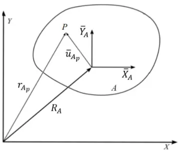
When studying complex systems, there are two systems of coordinates that can be used as a reference when defining the position, velocity, and acceleration of the bodies at all times. The first one is a global coordinate system, and the second is a local coordinate system. A global coordinate system is a reference for all bodies that constitute the system, while a local coordinate system is unique and different for each body. The more bodies are part of a system, the more local coordinate systems exist. Figure 2.2 gives an example of the difference between the two coordinate systems, where the global coordinate axes are defined by X and Y and the local ones by 𝑋̅𝐴 and 𝑌̅𝐴.
Figure 2.2 Global vs. Local coordinate system, adapted from (Nikravesh, Computer-Aided Analysis of Mechanical Systems, 1988)
9 The position of a particle P, belonging to the rigid body A, in the global coordinate system, can be expressed in the following way:
𝐫𝐴𝑝 = 𝐑𝐴+ 𝐀𝐴𝐮̅𝐴𝑝 (1)
where 𝐫𝐴𝑝 is the global position of a particle P, 𝐑𝐴 is the global position of the body where P
belongs, 𝐀𝐴 is the transformation matrix, and 𝐮̅𝐴𝑝 is the position of P relatively to the local coordinate system. The vector 𝐮̅𝐴𝑝is considered constant because the body A is considered as a rigid body.
The transformation matrix, 𝐀𝐴, can be expressed as:
𝐀𝐴 = [𝑐𝑜𝑠𝜃𝑠𝑖𝑛𝜃𝐴 −𝑠𝑖𝑛𝜃𝐴
𝐴 𝑐𝑜𝑠𝜃𝐴 ] (2)
where 𝜃𝐴 is the angle between the local coordinate system and the global one. The first and second
columns of matrix A represent the axes 𝑥̅ and 𝑦̅, respectively.
From the position of a particle, it is possible to obtain its velocity by differentiating the vector 𝐫𝐴𝑝 with respect to time:
𝐫̇𝐴𝑝 = 𝐑̇𝐴+ 𝐀̇𝐴𝐮̅𝐴𝑝 (3) where 𝐑̇𝐴 becomes the translational velocity of the body, and 𝐀̇𝐴 is the time derivative of the
rotation matrix, expressed as: 𝐀̇𝐴= [
−sin (𝜃𝐴)𝜃̇𝐴 −cos (𝜃𝐴)𝜃̇𝐴
cos (𝜃𝐴)𝜃̇𝐴 −sin (𝜃𝐴)𝜃̇𝐴
] = 𝜃̇𝐴𝐀𝜃,𝐴 (4)
𝜃̇𝐴 is the angular velocity of the particle. The particle’s velocity can then be expressed as follows:
𝐫̇𝐴𝑝 = 𝐑̇𝐴+ 𝜃̇𝐴𝐀𝜃,𝐴𝐮̅𝐴𝑝 (5) From the velocity it is also possible to obtain the acceleration, once again, by differentiating the previous equation with respect to time:
𝐫̈𝐴𝑝 = 𝐑̈𝐴− 𝜃̇𝐴
2𝐀
𝜃,𝐴𝐮̅𝐴𝑝+ 𝜃̈𝐴𝐀𝜃,𝐴𝐮̅𝐴𝑝 (6) where 𝐑̈𝐴 is the translational acceleration component, 𝜃̇𝐴2𝐀𝜃,𝐴𝐮̅𝐴𝑝 is the normal acceleration component, and 𝜃̈𝐴𝐀𝜃,𝐴𝐮̅𝐴𝑝 is the tangential acceleration component of the acceleration.
10
It is necessary to establish whether the study is to be made using dependent or independent coordinates. According to de Jalón and Bayo (2009), the first dilemma encountered when choosing a system of coordinates which may describe the motion by position, velocity, and acceleration is the problem of either adopting a set of independent coordinates, whose number coincides with the number of degrees of freedom (DOF) and is thereby minimal or adopting an expanded system of dependent coordinates.
The problem can be solved, no matter what type of coordinates is chosen, but the solutions obtained are not similar. Depending on what the problem and the specifications are, using dependent or independent coordinates will have an impact on the efficiency, computational cost, and easiness of the solutions proposed. For example, independent coordinates change all the time because of the movement, and, although the number of equations is minimal, the need to always find the most appropriate set of coordinates can affect the computational effort. Dependent coordinates, on the other hand, although giving a bigger number of equations, do not change for every time instant considered, and the same set of coordinates can be used during all the analysis. Constraint joints
Normally, in multibody systems, many different joints can be used to model the connection between bodies. The most common joints used are revolute and translational joints.
In planar systems, as the name says, translational joints only allow relative translational movement along one axis between the two bodies, meaning that only one DOF is available. The axis of relative translational movement is called the line of translation (Nikravesh, Planar Multibody Dynamics: Formulation, Programming and Applications, 2008). Revolute joints also allow only one DOF, but instead of being the movement along one axis, it is the rotation along one axis.
2.3
Kinematic Analysis
To perform any analysis of a system, the first thing to do is a kinematic analysis, where the focus is on the geometric aspects of the motion, regardless of the forces acting on the system. When performing a kinematic analysis, the input elements or input coordinates should be identified. Input elements are the ones whose position or motion is described, and input coordinates can be an angle or a distance to a reference point (de Jalón & Bayo, 2009).
To perform this analysis, the system’s DOF should first be identified, in order to establish and describe the kinematic relationships in terms of the DOF and their time derivatives. Knowing the existing constraints is also a critical part before performing this analysis.
11 The number of constraint equations is equal to the difference between the number of dependent coordinates and the number of DOF’s (𝑚 = 𝑛 − 𝑓) (de Jalón & Bayo, 2009). Therefore, for this system’s analysis, a formulation in dependent coordinates should be adopted.
For the system’s analysis in dependent coordinates, it is necessary to describe how the constraint conditions should be represented:
𝚽(𝐪, 𝑡) = 0 (7) Where 𝐪 represents the displacement’s matrix and 𝑡 represents the instant considered.
When imposing a displacement change to any constraint equation, it follows that:
𝚽(𝐪 + ∆𝐪, 𝑡) = 𝟎 (8) and by using the Taylor series development, the residual (displacement change) added to the generalized coordinates can be written as:
𝚽(𝐪 + ∆𝐪, 𝑡) = 𝚽(𝐪, 𝑡) +𝛛𝚽(𝐪,𝑡) 𝛛𝐪 ∆𝐪 + 1 2 𝛛𝟐𝚽(𝐪,𝑡) 𝛛𝐪𝟐 ∆𝐪 𝟐+ ⋯ (9)
the first order terms from the Tayler series expansion, because it is assumed to be sufficiently accurate, can be used to give a similar expression to eq (9):
𝚽(𝐪 + ∆𝐪, 𝑡) = 𝚽(𝐪, 𝑡) +𝛛𝚽(𝐪,𝑡)
𝛛𝐪 ∆𝐪 = 0 (10) 𝛛𝚽(𝐪,𝑡)
𝛛𝐪 is denoted as 𝐂𝐪 and is called the Jacobian Matrix. For any given system, the Jacobian
matrix is an 𝑚 ∗ 𝑛 sized matrix:
𝐂𝐪 = [( 𝜕𝐶1 𝜕𝑞1 𝜕𝐶1 𝜕𝑞2 ⋯ 𝜕𝐶1 𝜕𝑞𝑛 𝜕𝐶2 𝜕𝑞1 𝜕𝐶2 𝜕𝑞2 ⋯ 𝜕𝐶2 𝜕𝑞𝑛 ⋮ ⋮ ⋱ ⋮ 𝜕𝐶𝑚 𝜕𝑞1 𝜕𝐶𝑚 𝜕𝑞2 ⋯ 𝜕𝐶𝑚 𝜕𝑛)] (11)
where 𝐶𝑖 stands for any constraint equation and 𝑞𝑖 represents the parameter chosen.
The first step of the kinematic analysis is determining the locations and orientations of the different bodies, also known as position analysis. The position can be represented using a 𝐫. The second step, after knowing the displacement variables, is a velocity analysis. It is used to determine the velocities of the different bodies that make the system as functions of the time rate and the DOF’s. Velocity equations can be achieved by differentiating the position equations in order of time, being represented by 𝐫̇ . The third and final step is to perform the acceleration analysis. This analysis is also done by differentiating the previous equations in order of time to get the accelerations of the different bodies. Acceleration is represented by 𝐫̈. (Shabana, 2001).
12
The main difference between kinematic analysis and dynamic analysis is that the first one does not take into consideration the forces applied to the system while the second one does. Next, dynamic analysis is introduced.
2.4
Dynamic Analysis
A truly dynamic problem can be described as having more unknown dependent variables than independent geometric and driving constraint equations. Because of this, it is necessary to establish a dynamic equilibrium condition, taking into consideration the existing loads applied on the system. This dynamic condition leads to a system of second-order differential equations known as the equations of motion (de Jalón & Bayo, 2009).
All descriptions of forces acting on bodies can be associated to Newton (1642-1727), who wrote the three basic laws that guide dynamics:
1. principle of inertia: a particle, where the total sum of the forces applied is equal to zero, tends to maintain its state;
2. principle of force: the acceleration of a particle is proportional to the force applied, with the same direction as the applied force;
3. principle of action/reaction: for every force applied in one of a pair of interacting bodies, there is a reaction force with the same magnitude, opposite direction and collinear happening on the other body of the pair.
The author Sol proposes three steps for performing any dynamic analysis. First, the mass, the inertia tensor, and the body’s momentum need to be discussed. Then follows a description of the external loads and torques imposed on the system. And finally, the equations of motion are given (Sol, 1983). Sol also proposes three ways to get to the equations of motion: The Newton-Euler laws, the virtual work principle of d’Alembert, and the equations of Lagrange (Sol, 1983). There has been a lot of research about the pros and cons of the different definitions, regarding two major ways of performing the dynamic analysis, one using redundant coordinates and the other, using the system’s DOF’s. The first way leads to a bigger number of equations but gives a more general idea of the formulation and can achieve a sparse matrix structure (where most elements are equal to zero), while the second way leads to a much smaller number of equations, but the complexity increases with the appearance of different coefficients (Shabana, 2001).
Using either the Newton-Euler equations, the method of virtual work or Lagrange’s equations, it is possible to achieve the same result, which is the equations of motion that describe the body’s behaviour.
13 Principle of virtual work
First, it is useful to understand what the principle of virtual work is. This principle is used together with the principle of virtual displacement, and both are essential to derivate the equations of motion of a system. When applying a virtual displacement, the change of time, dt, is not taken into consideration.
When applying a virtual displacement to a body under the action of a force, a new vector appears, called the generalized external forces vector, expressed as Q. The virtual work done by the force applied to the body can be calculated as:
𝛿𝐖𝑒𝑥𝑡,𝐴= 𝛿𝐫𝐴𝑇𝐅𝐴 (12)
𝛿𝐫𝐴𝑇 = ( 𝛿𝐫𝐴
𝛿𝐪𝐴) 𝛿𝐪𝐴 (13) where A stands for a given body where the force is applied. The relation 𝛿𝐫𝐴𝑇 = (𝛿𝐫𝐴
𝛿𝐪𝐴) 𝛿𝐪𝐴 can
be written in a different way: 𝛿𝐫𝐴𝑇 = [𝐈 𝐀𝐴𝐮̅𝐴] [𝛿𝐑𝛿𝛉𝐴
𝐴] (14)
It is possible to rewrite eq (12) in a simpler way, using the relations given:
𝛿𝐖𝑒𝑥𝑡,𝐴= [𝛿𝐑𝐴 𝑇 𝛿𝛉𝐴 ] 𝑇 [𝐈 𝐀𝐴𝐮̅𝐴]𝑇𝐅𝐴= [𝛿𝐑𝐴 𝑇 𝛿𝛉𝐴 ] 𝑇 [𝐀 𝐅𝐴 𝐴𝐮̅𝐴𝐅𝐴] = [ 𝛿𝐑𝐴𝑇 δ𝛉𝐴 ] 𝑇 𝐐𝒆,𝐴 (15)
vector 𝐐𝒆,𝑨 is called the generalized forces vector of the force 𝐅𝑨. Vector 𝐐𝒆,𝑨 includes the
translational and rotational components.
Using the same principle, it is also possible to characterize the inertial forces applied to the body. They can be expressed as:
𝐅𝑖𝑛𝑒𝑟,𝐴= ∫ 𝜌𝐫̈𝑉 𝐴𝑑𝑉𝐴
𝐴 (16) The virtual work done by the inertial forces can be written as:
𝛿𝐖𝑖𝑛𝑒𝑟,𝐴= 𝛿𝐫𝐴𝑇𝐅𝑖𝑛𝑒𝑟,𝐴= ∫ 𝜌𝛿𝐫𝑉𝐴 𝐴𝑇𝐫̈𝐴𝑑𝑉𝐴 (17)
Using eq (13) to write the virtual displacement, eq (17) can be changed to: 𝛿𝐖𝑖𝑛𝑒𝑟,𝐴= ∫ 𝜌𝛿𝐪𝐴( 𝛿𝐫𝐴 𝛿𝐪𝐴) 𝐫̈𝐴𝑑𝑉𝐴 𝑉𝐴 = 𝛿𝐪𝐴 𝑇𝐐 𝑖𝑛𝑒𝑟,𝐴 (18)
14
From eq (18), the virtual displacement of a body can be described as the product of the transposed virtual displacements matrix 𝛿𝐪𝐴𝑇 with the generalized inertial forces vector acting on
the body, 𝐐𝑖𝑛𝑒𝑟,𝐴. The inertial forces (and consequently the inertial work) acting on these types
of systems can be despised when compared with the external forces applied. Principle of virtual power
This principle is similar to the principle of virtual work, with the only difference being the use of a virtual velocity instead of a virtual displacement. It can be used to solve the static equilibrium position problem. On the final equilibrium position, the virtual power of all the forces acting on the multibody should be zero.
First, a virtual velocity vector needs to be defined. It can be defined as a set of imaginary velocities at a stationary time that is consistent with the homogeneous form of the velocity constraint equations. This vector will have the denomination 𝐪̇∗. The velocity constraint equations can be driven from the equations of virtual displacements and imposing the virtual variation of the constraint to be zero:
𝚽̇ = 𝚽𝐪𝑇𝐪̇∗= [2𝑥 2𝑦] {𝑥̇ ∗
𝑦̇∗} = 0 (19)
where 𝚽̇ represents the virtual velocity constraints, 𝚽𝐪𝑇 is the displacement constraints transposed
matrix, and 𝑥̇∗and 𝑦̇∗ are the virtual velocities according to the X and Y axis, respectively. Using 𝐪̇∗ as a set of n dependent virtual velocities, the principle of virtual power can be presented as:
𝐖∗ = ∑ 𝐅 𝑖𝐪̇𝑖∗ 𝑛
𝑖=1 = 𝐪̇∗𝑇𝐅 = 0 (20)
where F is the vector of all the forces that produce virtual power, including the inertial ones: 𝐅 = 𝐌𝐪̈ − 𝐐 (21) M is the mass matrix of a system:
𝐌𝑖= [𝐦𝑅𝑅𝑖 𝐦𝑅𝜃𝑖
𝐦𝑅𝜃𝑖 𝐦𝜃𝜃𝑖
] (22)
The term 𝐦𝑅𝑅𝑖 is the one associated with the body’s translational movement and is a constant
diagonal matrix: 𝐦𝑅𝑅𝑖 = [ 𝑚𝑖 0 0 0 𝑚𝑖 0 0 0 𝑚𝑖 ] (23)
where 𝑚𝑖 represents the total mass of the body. The next term, 𝐦𝑅𝜃𝑖 , represents the inertia coupling between the translation and rotation of the body and can be defined as:
15 𝐦𝑅𝜃𝑖 = −𝐀A∫ 𝜌𝑖𝐮̃𝑖𝑑𝑉𝑖𝐆̅𝑖 (24)
where 𝐀A is the transformation matrix, 𝐮̃𝑖 is the distance between the coordinate system and the
body’s centre of mass and 𝐆̅𝑖 is a matrix that depends on the Euler parameters. The Euler
parameters are used to describe a finite rotation from the body along an arbitrary axis, its values are usually low (Mevea assumes the rotation to be minimum), the matrix 𝐦𝑅𝜃𝑖 tends to be a null matrix (full of zeros).
Finally, the term 𝐦𝜃𝜃𝑖 is associated with the rotational coordinates of the body reference, and can be written as:
𝐦𝜃𝜃𝑖 = 𝐆̅𝑖T𝐈̅𝜃𝜃𝑖 𝐆̅𝑖 (25)
where 𝐈̅𝜃𝜃𝑖 is the inertia tensor of the rigid body, defined as:
𝐈̅𝜃𝜃𝑖 = [
𝑖11 𝑖12 𝑖13
𝑖22 𝑖23
𝑠𝑦𝑚 𝑖33
] (26)
Note: This mass matrix definition is for a spatial system. Although using, for all the kinetic and dynamic analyses, planar systems, the system considered as a study case is a spatial one, hence the necessity of introducing the mass matrix for spatial systems. For planar ones, the final mass matrix will be an index four square matrix.
Equation (21) can lead to a set of equilibrium equations where the internal constraint forces are not considered, although these equations should be considered in a state of equilibrium. In order to take into consideration these equations, it is necessary to add a set of forces in the direction of the constraint violations (𝚽𝐪𝑇𝛌) where the columns of 𝚽𝐪𝑇 (rows of 𝚽𝐪) give the
direction of the constraint forces and 𝛌 is the vector of their magnitudes. Because the virtual velocity vector 𝐪̇∗ belongs to the null space of 𝚽
𝐪, the product (𝐪̇∗𝚽𝐪𝑇𝛌) is equal to zero and
therefore can be added to the equation (20), giving the complete set of force equilibrium equations:
𝐖∗ = 𝐪̇∗𝑇(𝐌𝐪̈ − 𝐐 + 𝚽𝐪𝑇𝛌) = 0 (27)
And consequently:
𝐌𝐪̈ + 𝚽𝐪𝑇𝛌 = 𝐐 (28)
Therefore, the virtual power of the forces acting on a multibody system can be written as: 𝐪̇∗𝑇(𝐌𝐪̈ − 𝐐) = 0 (29)
16
It is possible to find the 𝑚 values of the vector 𝛌. This vector establishes the magnitude of the constraint forces, so that:
𝐌𝐪̈ + 𝚽𝐪𝑇𝛌 = 𝐐 (30)
where now the vector Q contains the external forces plus all the velocity dependent inertial terms. Note: The expressions and definitions for the principles of virtual work and virtual force are adapted from (de Jalón & Bayo, 2009).
Method of the Lagrange multipliers
Equation (30) represents a set of 𝑛 equations with a total of (𝑛 + 𝑚) unknown variables: 𝑛 variables belonging to vector 𝐪̈ and 𝑚 variables, belonging to the vector 𝛌. To solve the problem, it is necessary to have the same number of equations and number of unknowns, so there is a need to supply 𝑚 more equations. To do this, acceleration kinematic equations can be added. These are obtained by differentiating the constraint equations (7) twice with respect to time:
𝚽𝐪𝐪̈ = −𝚽̇𝑡− 𝚽̇𝐪𝐪̇ = 𝐜 (31)
The vector 𝐜 appears as a form of simplification of the previous equation. Writing equations (30) and (31) together, makes it possible to introduce the following matrix system:
[𝐌 𝚽𝐪 𝑇 𝚽𝐪 𝟎 ] { 𝐪̈ 𝛌} = { 𝐐 𝐜} (32) which is a system with (𝑛 + 𝑚) equations with (𝑛 + 𝑚) unknowns. This system can be used to solve both accelerations and Lagrange multipliers (de Jalón & Bayo, 2009).
Semi recursive formulation
This type of formulation allows the dynamic analysis of a body to be done more efficiently, being used in computational analysis. It requires the system to have a tree structure (see figure 2.3). The main advantages of using recursive definitions are an easier derivation of the equations of motion, easier software coding and debugging, and reduced computational effort.
Using the semi recursive formulation, the equations of motions can be written as follows: 𝐪̈ = 𝑓(𝐪, 𝐪̇, 𝑡) (33)
17 where 𝐪̈ has a reduced size because it only contains relative coordinates of one body respectively to an adjacent body of the system. For this type of definitions, only reduced matrices need to be inverted, which requires less computational effort than having to invert large matrices (the integration itself does not take too much computational effort but the inversion of large-sized matrices does). As a result, only small equations of similar type as equation (20) need to be integrated.
Semi recursive formulation uses the relationships between an arbitrary pair of contiguous bodies belonging to the same system. The pairs interact through a joint. Considering that all bodies are connected to each other by any type of joints, a tree structure can be considered, so that the formulation can be applied.
A tree structure is also considered an open loop chain system of bodies. Figure 2.3 exemplifies a tree structure of a multibody system. The body 𝐵1 is considered the base of the
system and so on. The bigger the number of bodies between body𝐵𝑖 and body 𝐵1, the bigger the
number assigned to the body 𝐵𝑖 (Slaats, 1991).
Figure 2.3 Tree structure of a multibody system, adapted from (Slaats, 1991)
Semi recursive formulation starts by describing the kinematics associated with each arbitrary pair. Figure 2.4 exemplifies an arbitrary pair of bodies, 𝐵𝑗−1 and 𝐵𝑗, connected by an
arbitrary joint. X, Y, and Z represent the global coordinate reference axis, while 𝑥̅𝐵𝑗−1, 𝑦̅𝐵𝑗−1, and 𝑧̅𝐵𝑗−1 represent the local coordinate reference axis at 𝐵𝑗−1, located in its centre of mass. Points P and Q represent the location of the joint in both bodies. Vector 𝐝𝐣−𝟏,𝐣 shows the relative
18
Figure 2.4 Arbitrary pair of bodies Bj-1 and Bj, adapted from
(Jaiswal;Islam;Hannola;Sopanen;& Mikkola, 2018)
The global position vector of body 𝐁𝑗, 𝐫𝑗, global velocity vector, 𝐫̇𝑗, and global
acceleration vector, 𝐫̈𝑗 can be written as:
𝐫𝑗= 𝐑𝑗−1+ 𝐀𝑗−1𝐮̅𝑗−1+ 𝐝𝑗−1,𝑗 (34)
𝐫̇𝑗= 𝐑̇𝑗−1+ 𝜃̇𝑗−1𝐀𝑗−1𝐮̅𝑗−1+ 𝐝̇𝑗−1,𝑗 (35)
𝐫̈𝑗= 𝐑̈𝑗−1− 𝜃̇𝑗−12 𝐀𝑗−1𝐮̅𝑗−1+ 𝜃̈𝑗−1𝐀𝑗−1𝐮̅𝑗−1+ 𝐝̈𝑗−1,𝑗 (36)
The angular velocity of the body 𝐵𝑗, 𝛚𝑗, and its angular acceleration, 𝛚̇𝑗, can be written
is terms of the global frame of reference, which means, in terms of the global angular velocity, 𝛚𝑗−1, and the global angular acceleration, 𝛚̇𝑗−1, respectively:
𝛚𝑗= 𝛚𝑗−1+ 𝛚𝑗−1,𝑗 (37)
𝛚̇𝑗= 𝛚̇𝑗−1+ 𝛚̇𝑗−1,𝑗 (38)
with the index (𝑗 − 1, 𝑗) meaning the velocity and acceleration of the body 𝐵𝑗 with respect to the
body 𝐵𝑗−1.
Using the principle of virtual work in matrix form and the kinematic analysis presented above, the equations of motion for the body 𝐵𝑗 can be written:
{𝐪̇𝑗∗𝑇 𝛚𝑗∗𝑇} ([ 𝐌𝑗𝐈3 0 0 𝐀𝑗𝐉𝟎(𝐀𝑗𝑇) ] [𝐑̈𝑗 𝛚̇𝑗 ] + [𝛚̃ 0 𝑗𝐀𝑗𝐉𝟎(𝐀𝑗𝑇)𝛚𝑗] − [ 𝐅𝑗 𝐓𝑗]) = 0 (39)
19 Where 𝐪̇𝑗∗ and 𝛚𝑗∗ are, respectively, the virtual translational velocity and the virtual angular velocity, 𝐌𝑗 is the mass matrix of the body 𝐵𝑗, 𝐈3 is the index three identity matrix, 𝐉𝟎 is the
rotation inertia tensor, 𝐀𝑗 is the rotation matrix, 𝛚̃𝑗 is the skew-symmetric matrix of 𝛚𝑗, and 𝐅𝑗
and 𝐓𝑗 are forces and torques applied to the body 𝐵𝑗, respectively.
For the entire system, the equations of motions can be written like equation (28): 𝐪̇∗T(𝐌𝐪̈ − 𝐐 + 𝚽
𝐪𝑇𝛌) = 0 <=> 𝐪̇∗𝑇(𝐌𝐪̈ − 𝐐 + 𝐂) = 0 (40)
𝚽𝐪𝑇𝛌 is the quadratic velocity and it can be represented by the letter value 𝐂. This system
of equations can shorten by using relative joint coordinates. Global velocities and relative joint velocities can relate by using the velocity transformations matrix, 𝐑:
𝐪̇ = 𝐑𝐳̇ (41) where 𝐳̇ is the relative joint velocities vector. The accelerations, 𝐪̈ can be obtained by differentiating the previous system in order of time:
𝐪̈ = 𝐑𝐳̈ + 𝐑̇𝐳̇ (42) where 𝐳̈ is the relative joint acceleration vector and 𝐑̇ is the time derivative of 𝐑.
By substituting the equations (41) and (42) into equation (40), the equations of motion can be expressed as:
𝐳̇∗𝑇(𝐑𝑇𝐌𝐑𝐳̈ + 𝐑𝑇𝐌𝐑̇𝐳̇ + 𝐑𝑇𝐂 − 𝐑𝑇𝐐) = 0 (43)
Because this equation is valid for any arbitrary vector of independent velocities, 𝐳̇∗ can
be eliminated from the expression and the equations of motion can be written in a simpler way: 𝐑𝐓𝐌𝐑𝐳̈ = 𝐑T(𝐐 − 𝐂) − 𝐑T𝐌𝐑̇𝐳̇ (44)
Note: The explanation presented in this subchapter is adapted from (Jaiswal;Islam;Hannola;Sopanen;& Mikkola, 2018)
2.5
Numerical Integration
Dynamic analysis of constrained multibody systems leads to a set of differential algebraic equations (DAE). Because those equations are very difficult to solve analytically, researchers have tried to seek numerical methods to approximate the solutions at discrete times (𝑡1, 𝑡2, 𝑡3,
…). The amount of time passed between discrete times is considered constant (for the method used) and is defined as a time step ∆𝑡 .To approximate the solution at different discrete times, these equations need to be transformed into second order differential equations (ODE), and after that into first order ODE’s, so that the numerical integration can be fast and accurate.
20
The numerical integration can be made using various computational tools and it is becoming an important part of computational dynamics due to the easiness to implement as well as faster implementation time.
Second order differentials like the acceleration equation can be expressed as:
𝐪̈ = 𝐅(𝑡, 𝐪, 𝐪̇) (45) This equation’s solutions also need to satisfy the initial conditions 𝐪(𝑡0) = 𝐪𝟎 and
𝐪̇(𝑡0) = 𝐪̇𝟎. Most computer software tools try to solve this type of equations by turning them into
first order ODE’s and then solving them. The transformation can be done by substituting the variable 𝐪̇ for a first order one, 𝐬, (𝐪̇ = 𝐬). That way, a new ODE appears instead of equation (45): 𝐬̇ = 𝐟(𝑡, 𝐪, 𝐬) (46) Introducing 𝐲𝐓≡ {𝐪T, 𝐬T} as a new vector variable that includes 𝐪 and 𝐬, equation (46) can be rewritten in a simpler way:
𝐲̇ = 𝐟(𝑡, 𝐲) (47) Given t and y, the value of 𝐲̇ is calculated and consequently, the accelerations end up being calculated. This process is called function evaluation (de Jalón & Bayo, 2009).
Figure 2.5 resumes the process of numerical integration in dynamic analysis. It is important to notice that numerical integration process occurs until the end of the analysis time. The instant where the numerical integration occurs is represented by the letter t. When the numerical integration happens, the function evaluation checks if the instant is higher or equal than the total time. If it is not higher or equal, the next instant is considered by adding an infinitesimal amount of time, dt, to the previous time instant.
21 Figure 2.5 Numerical integration in dynamic analysis
Runge-Kutta Method
This method works as a numerical integration method to transform the DAE’s into ODE’s and solve them. It was created due to the low accuracy levels of Euler’s method and the difficulty of obtaining the higher order derivatives 𝐟(𝑡, 𝐲) in Taylor’s series. Although Euler’s method easiness to implement, it requires the time steps used to be very small, making the round-up errors increase and consequently making this method useless (de Jalón & Bayo, 2009).
Runge-Kutta method works by doing function evaluations instead of computing higher order derivatives. By knowing information about 𝑡 and 𝑦 it computes the value of 𝑦̇ for each time step. This reduces the round up errors (Flores, 2015).
Starting with the Euler’s method, the equation that provides the solution for each 𝑦𝑖 is presented as:
𝑦𝑖+1 = 𝑦𝑖+ ∆𝑡𝑓(𝑡𝑖, 𝑦𝑖) + 𝑂(ℎ2) (48)
where 𝑂(ℎ2) represents the local truncation error. The method’s order and accuracy can be
specified by its local truncation order’s error. For a truncation error with order 𝑂(ℎ𝑝+1), the
method’s order will be 𝑝. It is easy to understand that the Euler’s method is a first order method. The higher the order of the method, the more accurate it becomes.
22
To increase the order of the Euler’s method, a new method was developed, called the Runge-Kutta second order method which can also be called the improved Euler’s method:
𝑦𝑖+1 = 𝑦𝑖+ ∆𝑡 2(𝑘1+ 𝑘2) + 𝑂(ℎ 3) (49) 𝑘1= 𝑓(𝑡𝑖, 𝑦𝑖) (50) 𝑘2= 𝑓(𝑡𝑖+ ∆𝑡, 𝑦𝑖+ ∆𝑡𝑘1) (51)
This method requires two function evaluations for each time step, meaning two solutions of the equations of motion to obtain the accelerations at any given time step. It is important to notice that 𝑘1 does not depend on 𝑘2. Figures 2.6 and 2.7 serve as an example for the Euler’s
method and the Runge-Kutta second order method. From the first look it is possible to understand the difference between both in terms of accuracy. Runge-Kutta methods use more function evaluations for each time step, reducing the round-up errors. For the second order method (figure 2.7), between points 𝑡𝑖 and 𝑡𝑖+1, the midpoint derivative is used to increase accuracy. In both
figures, the time instants are represented by the letter X.
Figure 2.6 Euler's method, adapted from (Press;Teukolsky;Vetterling;& Flannery, 1992)
Figure 2.7 Rung-Kutta second order method, adapted from (Press;Teukolsky;Vetterling;& Flannery, 1992)
23 One of the most used methods used in multibody dynamics analysis is the Runge-Kutta fourth order method. As the name says, it is a fourth order method, meaning that it should be more accurate than the previous two methods presented. It allows a bigger timestep to be used (and for a timestep twice as big as the one used in the second order method the accuracy is the same) with the biggest difference being the requirement of four function evaluations for each time step. This method can be expressed as:
𝑦𝑖+1 = 𝑦𝑖+ ∆𝑡 6(𝑘1+ 𝑘2+ 𝑘3+ 𝑘4) + 𝑂(ℎ 5) (52) 𝑘1= 𝑓(𝑡𝑖, 𝑦𝑖) (53) 𝑘2= 𝑓 (𝑡𝑖+ ∆𝑡 2 , 𝑦𝑖+ ∆𝑡 2 𝑘1) (54) 𝑘3= 𝑓 (𝑡𝑖+ ∆𝑡 2 , 𝑦𝑖+ ∆𝑡 2 𝑘2) (55) 𝑘4= 𝑓(𝑡𝑖+ ∆𝑡, 𝑦𝑖+ ∆𝑡𝑘3) (56)
Now the values of the different 𝑘𝑖+1 depend on the previous values. This method does
not provide an estimate of the local error, so it is difficult to know if the time step being used is the correct one. Because of the reduced computational cost, it does not a problem to try different time steps. Figure 2.8 shows the four function evaluations between time steps, ordered by numbers. The first evaluation occurs at the initial point of the time step, while to next two ones occur in the midpoints. The final one should occur in the final point of the time step. These evaluations can be considered as tangents to the actual function.
Figure 2.8 Fourth-order Runge-Kutta method, from (Press;Teukolsky;Vetterling;& Flannery, 1992)
Note: the information and equations presented in this sub-chapter are adapted from (Press;Teukolsky;Vetterling;& Flannery, 1992), (de Jalón & Bayo, 2009), and (Flores, 2015).
Mevea software uses a semi-recursive formulation and a Runge-Kutta fourth order method to perform the system’s dynamic analysis.
24
2.6
Collision and contact modelling
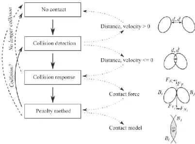
When performing a simulation using complex systems, collisions should be taken into consideration. The model and the simulation need to be realistic, prohibiting the interpenetration of bodies. It is necessary to determine when contact happens, how many bodies are colliding and what the collision response should be. To understand this, two major steps are considered: contact detection and collision response. Contact detection is considered the most important step. It relies on the geometry of the bodies to be accurate. The collision geometry needs to be simple, so that the software can return the possibility of when and where the collision is going to happen. Figure 2.9 shows the difference in a body’s model geometry and the one used for contact detection. It is possible to notice the differences between the model and the collision model, where the geometry has rectangular shapes. Contact response is what keeps the bodies from entering each other. It analyses the bodies and their properties, like contact forces, geometric properties and relative velocities. (Baharudin;Rouvinen;Korkealaasko;& Mikkola, 2014).
Figure 2.9 Simulation model vs. collision model
One of the existing theories for analyzing collisions in real time simulation is the Penalty method. It is also known as the soft contact method because it allows small penetrations between bodies and adds a temporal spring damper. Figure 2.10 resumes how this method works for collision detection. Vectors 𝐝 and 𝐝̇ are the distance and velocity between the two bodies, while 𝐅𝑁 and 𝐅𝑇 are the normal and tangent forces. When 𝐝 and 𝐝̇ are equal or less than zero the collision
occurs and the collision response method starts to work (Baharudin;Rouvinen;Korkealaasko;& Mikkola, 2014).
25 Figure 2.10 Collision detection between two bodies, from
(Baharudin;Rouvinen;Korkealaasko;& Mikkola, 2014)
The collision can be described using a global frame of reference and two bodies like it is showed in figure 2.11. The vectors 𝐫𝑖 and 𝐫𝑗 represent the location of the contact point of both
bodies with respect to the global frame. The distance between the two bodies is 𝐝𝑝.
Figure 2.11 Contact between two bodies, adapted from (Baharudin M. , 2016)
𝐝𝑝 can be calculated as:
𝐝𝑝= 𝐫𝑗− 𝐫𝑖 (57)
It is possible to calculate the normal vector at the contact point, 𝐧: 𝐧 =∥𝐝𝐝𝑝
𝑝∥ (58) and with the normal vector, the location of the collision, 𝐝, can be known:
26
The relative velocity of the collision can also be calculated:
𝐯𝑛= 𝐧T(𝐫̇𝑗− 𝐫̇𝑖) (60)
In order to define the contact forces, a spring and a damper are added. That collision force can be expressed as:
𝐅 = −𝐾𝐱 − 𝑆(𝐧𝐯𝑛) (61)
where 𝐾𝐱 represent the spring’s force and 𝑆 is the damping coefficient. It is important to choose the coefficients’ values right to obtain valid collision results.
Note: The information and expressions here presented are adapted from (Baharudin;Rouvinen;Korkealaasko;& Mikkola, 2014).
2.7
Hydraulic circuit
When using a system with a hydraulic circuit in it, it becomes necessary to perform also an analysis of this sub-system. When modelling and analyzing hydraulic circuits, there are two important properties to take into consideration: viscosity and bulk modulus.
Viscosity can be defined as a measure of the fluid’s resistance to deformation by shear or tensile stress, while the bulk modulus can be defined as a measure of the fluid’s resistance to compression, or in the other words, it can be defined as the infinitesimal pressure increase related to the infinitesimal volume decrease. The bulk modulus, 𝐵, can be expressed by the following expression and has a typical value of 1500 Mpa, for oil:
𝐵 = −𝑑𝑝𝑑𝑉 𝑉
= −𝑉𝑑𝑝
𝑑𝑉 (62)
Figure 2.12 shows a unit sized hydraulic volume, used as an infinitely stiff container to exemplify the bulk modulus. The volume is compressed by a force, causing a −𝑑𝑉 change. That change causes the pression to increase 𝑑𝑝.
27 When using multiple volumes, the system has multiple bulk modulus. This combined effect of the different bulk modulus is called effective bulk modulus, 𝐵𝑒 (Mikkola, Week 9-18moo,
2018).
When applying a force to a certain hydraulic volume, the oil compresses while the container expands. The starting volume can be expressed as:
𝑉𝑡 = 𝑉1= 𝑉𝑐1 (63)
where 𝑉1 is the initial fluid volume, and 𝑉𝑐1 is the initial volume of the container. The means it
does not matter if the volume chosen is the volume or the container one. When imposing volume changes, 𝑑𝑉𝑡, it can be written:
𝑑𝑉𝑡= −𝑑𝑉1+ 𝑑𝑉𝑐1 (64)
The oil used when modelling hydraulic circuits is compressible and it behaves like a spring. Different oils have different properties.
For mobile machines, it is possible to use the lump fluid theory, explained in this chapter. Flow types
The flow type is a very important factor to take into consideration when working with hydraulic circuits. The flow can be divided into two types: laminar and turbulent.
Laminar flow occurs when the fluid moves smoothly between layers. There are no movements in another direction different from the direction of the movement. On the other hand, turbulent flow occurs when the fluid’s particles have no specific trajectory and have different velocities Figure 2.13 gives an example of the two types of flow.