Universidade de Aveiro 2020
Departamento de Economia, Gestão, Engenharia Industrial e Turismo
Ana Beatriz Santos
Ferreira Rocha
Substituição de moeda e previsão da inflação em
Angola: comparação entre diferentes agregados
monetários
Currency substitution and inflation forecast in
Angola:
comparison
of
alternative
monetary
aggregates
Dissertação apresentada à Universidade de Aveiro para cumprimento dos requisitos necessários à obtenção do grau de Mestre em Economia, realizada sob a orientação científica do Doutor António Miguel Amôedo Lebre de Freitas, Professor Auxiliar do Departamento de Economia, Gestão, Engenharia Industrial e Turismo da Universidade de Aveiro.
o júri
Presidente Prof. Doutora Mara Teresa da Silva Madaleno
Professora Auxiliar, Universidade de Aveiro
Prof. Doutor Álvaro Pinto Coelho de Aguiar
Professor Associado, Faculdade de Economia da Universidade do Porto
Prof. Doutor António Miguel Amôedo Lebre de Freitas
agradecimentos Ao professor Miguel Lebre de Freitas, por este ano desafiador e de aquisição de conhecimento.
Ao curso de Economia, por fazer de Aveiro a minha casa.
À professora Mara Madaleno, que forneceu as aulas essenciais para a metodologia neste trabalho e está sempre pronta a ajudar.
Ao Rúben, por ser um exemplo a seguir.
palavras-chave Procura de moeda, Angola, Substituição de moeda, Inflação
resumo O objetivo principal deste estudo é identificar uma função procura de moeda
estável para Angola e comparar o poder de previsão de diferentes agregados monetários relativamente à inflação. Com dados mensais desde 2012:01 até 2019:01 foi estimado um Vector Error Correction Model onde foram utilizadas especificações alternativas no processo de estimação. Foi também estimado um modelo Autoregressive Distributed Lag para prever a inflação no curto prazo. Os resultados sugerem que existe substituição de moeda em Angola levando à instabilidade da função procura de moeda. No entanto, também é possível verificar que este problema pode ser superado através do uso de agregados monetários mais amplos que incluam depósitos em moeda estrangeira.
keywords Money Demand, Angola, Currency Substitution, Inflation
abstract The main purpose of this paper is to identify a stable money demand function
for Angola. Using monthly data from 2012:01 until 2019:01, we run a Vector Error Correction model, for the long-run relationships experimenting with different monetary aggregates. Then, an Auto Regressive Distributed Lag model is used to access the forecasting power of the corresponding excess liquidities regarding the inflation rate. The results indicate that there is currency substitution in Angola, but instability of money demand can be overcome by using broader monetary aggregates that include foreign currency deposits.
Index
Index ... i
Figure Index ... ii
Table Index ... iii
Acronym List ... iv
1. Introduction ... 1
2. Literature Review ... 3
2.1 Angola, Money Targeting and Currency Substitution ... 3
2.2 Theoretical Background on Money Demand with CS ... 5
2.3 Theoretical Model: Money Demand Function ... 6
3. Empirical Strategy and Data... 9
3.1 The Model ... 9 3.2 Data ... 9 3.3 Unit Roots ... 11 3.4 Estimation Method ... 12 4. Empirical Results ... 13 4.1 Cointegration Analysis ... 13
4.2 ARDL estimation and inflation forecast ... 17
5. Conclusions ... 21
References ... 23
Figure Index
Figure 1 - Degree of dollarization in Angola ... 4 Figure 2 - Variables used in the empirical analysis... 10 Figure 3 - Cointegration graphs... 26
iii
Table Index
Table 1 - Unit Roots Test ... 11
Table 2 - Johansen Cointegration Test and VECM results (part 1) ... 14
Table 3 - Johansen Cointegration Test and VECM results (part 2) ... 15
Table 4 - Restrictions imposed to previous estimations ... 17
Table 5 - ARDL estimation results of monthly inflation ... 18
Table 6 - ARDL estimation results when a dummy variable is included ... 19
Table 7 – Forecast evaluation ... 20
Table 8 - VECM Heteroskedasticity test ... 25
Table 9 - Chow Breakpoint Test ... 25
Acronym List
ADF – Augmented Dickey-Fuller AIC – Akaike Information Criterion ARDL – Auto Regressive Distributed Lag BNA – National Bank of Angola
CPI – Consumer Price Index CS – Currency Substitution CUSUM – Cumulative Sum
CUSUMQ – Cumulative Sum of Squares FCD – Foreign Currency Deposits GDP – Gross Domestic Product INE – National Statistics Institute LR – Likelihood-ratio
LSM – Liquidity Services Model PBM – Portfolio Balance Model USA – United States of America VAR – Vector Autoregressive
1. Introduction
In 2018, Angola adopted a new monetary policy regime, where the National Bank of Angola (BNA) controls directly the growth of the national monetary base (as the operational variable) (Banco Nacional de Angola, 2019) and indirectly the monetary aggregate M2 (as the intermediate goal) to insure the stability of prices in the medium and long run. The main reasoning underlying this strategy is the fact that inflation and the quantity of money have a long run relationship (Banco Nacional de Angola, 2018). Nevertheless, this strategy will only be effective if money demand is stable (Hossain, 2010).
Due to history of high inflation rates, Angola is a dollarized economy. If the opportunity cost of holding domestic money depends on the return of holding another currency, then domestic money demand will become unstable depending on the size of substitutability between the currencies. By the literature, currency substitution (CS) may destabilize domestic money demand, consequently reducing the effectiveness of money targeting (Calvo & Vegh, 1992).
Based on this, a question arises in whether the national monetary base is the appropriate monetary aggregate to target, or should a broader monetary aggregate be used instead?
To answer this question we estimate a money demand function for Angola experimenting with alternative monetary aggregates. A vector error correction model (VECM) estimation is computed and, afterwards, by taking the excess liquidities, an autoregressive distributed lag (ARDL) and a forecast analysis are made in order to check which measure of excess liquidity has more power predicting the price level. Excess liquidity is defined as the difference between the observed and the equilibrium monetary aggregates (Dreger & Wolters, 2010). We find evidence of currency substitution when considering narrow real money balances, such as the national monetary base. The same does not happen when using broader monetary aggregates, suggesting that CS is internalized. In this way, the money demand function becomes more reliable when broader monetary aggregates are used in the monetary policy formulation (Miles, 1978, 1981). In the forecast analysis, the results suggest that the model using the real broader M2 has a better forecasting power than the others.
The remaining of this study is organized as follows. Section 2 presents a brief revision of the literature as well as the theoretical model that underlies our money demand specification for Angola. Section 3 describes the variables and the methodology used in the empirical analysis. The estimation results are examined in section 4. By last, the conclusion is in section 5.
2. Literature Review
2.1 Angola, Money Targeting and Currency Substitution
Although, nowadays, most developed countries achieves price stability by conventionally controlling the interest rate (Dalziel, 2002), in the 1970s many Central Banks were targeting money (Federal Reserve Bank, 2018). The idea underlying this was that Central Banks kept inflation low and steady by keeping the money supply growth low and steady as well (Hossain, 2010), this comes from the classical view in which Friedman stated “inflation is always and everywhere a monetary phenomenon” (as cited in Hossain, 2010). When the United States of America (USA) came across a two digits inflation, in the end of 1970s, the monetarism was seen as the only way to achieve price stability. In 1979, the Federal Reserve stopped controlling the interest rate and decided to implement a “monetarist experiment” (Samuelson & Nordhaus, 2010). This experiment had success in stabilizing output and reducing inflation, which in two years reduced 9 percentual points. Albeit these results seemed quite satisfactory, the velocity of money became very unstable in the 1980s and was no longer predictable as monetarists defended. All these events led to the discrediting of monetarism, making the Federal Reserve to implement, in 1990, the interest rate as the main instrument to obtain price stability (Samuelson & Nordhaus, 2010).
Setting the interest rate as the main tool of monetary policy would not work in Angola as it presumes a developed financial system (Banco Nacional de Angola, 2018). Still, a question arises concerning the stability of money demand in developing countries whereas the problem of money demand instability is even more severe, since there is a tendency for economic agents to partially replace domestic currency by foreign currency in the basic functions of money (Calvo & Vegh, 1992), particularly, as store of value and medium of exchange (Freitas & Veiga, 2006; Giovanni & Turtelboom, 1992). When this occurs the country is in the presence of currency substitution. Usually, what happens is that domestic money is no longer seen as safe and as a “safety precaution” individuals act in order to protect their purchasing power (Prock, Soydemir, & Abugri, 2003).
Currency substitution has an important role when it comes to conduct monetary policy (Batten & Hafer, 1984; Chaisrisawatsuk, Sharma, & Chowdhury, 2004; Cuddington, 1983; Genc, Sahin, & Erol, 2005; Owoye & Onafowora, 2007). As pointed out by Batten & Hafer (1984), this phenomenon may deliver an unstable domestic money demand, undermining the monetary authority’s role in maintaining an efficient and independent policy. If the opportunity cost of holding domestic money depends on the return of holding another currency (exchange rate depreciation), then domestic money demand will become unstable depending on the size of substitutability between the currencies. That is, if depreciation of exchange rate happens and individuals resort to foreign currency as substitute of domestic currency, then this will negatively
4
impact the demand for domestic money (Calvo & Vegh, 1992; Mckinnon, 1982; Prock et al., 2003).
This phenomenon should be taken into account in the formulation of monetary policy. Miles (1978, 1981) argue that even that CS tend to deliver an unstable domestic money demand, if a broader monetary aggregate is applied in the monetary policy as the main instrument, the money demand function can become more reliable than by using a narrow monetary aggregate, since there is the possibility of the currency substitution effects to cancel out. Thus, if individuals can choose between national currency and foreign currency, then the real monetary aggregate that will determine prices is broader, including not only the national money, but as well the foreign money in the economy.
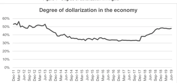
When it comes to Angola, in 2001, the deposits in foreign currency represented 82% of the total amount, leading the BNA to state a framework of effective financial dollarization of the economy (Banco Nacional de Angola, 2014). Even though the BNA started a de-dollarization process, the levels of dollarization are still quite high, the percentage of deposits in foreign currency in Angola represents, in April 2019, almost 50% of the total banking deposits (figure 1). This evidence is supportive of currency substitution in Angola, giving rise to some controversy regarding the monetary policy implemented in the beginning of 2018.
Notes: Own elaboration using data from Banco Nacional de Angola (2020). 0% 10% 20% 30% 40% 50% 60% D e c -1 1 Mar -1 2 J u n -1 2 S e p -1 2 D e c -1 2 Mar -1 3 J u n -1 3 S e p -1 3 D e c -1 3 Mar -1 4 J u n -1 4 S e p -1 4 D e c -1 4 Mar -1 5 J u n -1 5 S e p -1 5 D e c -1 5 Mar -1 6 J u n -1 6 S e p -1 6 D e c -1 6 Mar -1 7 J u n -1 7 S e p -1 7 D e c -1 7 Mar -1 8 J u n -1 8 S e p -1 8 D e c -1 8 Mar -1 9 J u n -1 9
Degree of dollarization in the economy
2.2 Theoretical Background on Money Demand with CS
To derive money demand functions in light of currency substitution, two main models are usually discussed by the literature. One is the Portfolio Balance Model (PBM) (Branson & Henderson, 1984; Cuddington, 1983; Zervoyianni, 1992) and the other is the Liquidity Services Model (LSM) (Bergstrand & Bundt, 1990; Miles, 1978; Mizen & Pentecost, 1994; Smith, 1995; Thomas, 1985).
Cuddington (1983) extends the standard PBM integrating currency substitution. According to this approach, the economic agent is allowed to hold their wealth in the form of domestic money, domestic bonds, foreign bonds and foreign money. Gross substitutability is assumed, leading to money demand functions that depend positively on income and negatively on the return of each alternative asset. The focus of the PBM in light of CS is the coefficient of the exchange rate depreciation, since this is the one that will show the existence or not of CS (Smith, 1995).
This approach has been criticised, since the model does not explain why individuals hold money. The Liquidity Services Model is used as an alternative model, that distinguishes itself from the PBM, because it accounts for the specific role of money. Thomas (1985) presented an expected utility maximizing model contradicting the PBM by showing that exchange rate depreciation does not impact money demand. Instead, the only opportunity costs that impact money demand are the interest rates (both domestic and foreign), that represent user costs into the production of money services. Fundamentally, in the LSM, instead of a one-stage allocation of wealth, there will be a sequential allocation, with two-stages. In the first-stage, individuals divide their wealth between money and other assets, then, in the second-stage they divide it between different types of money or bonds (i.e. domestic and foreign) depending on the choices in the first stage (Mizen & Pentecost, 1994). This two-stage allocation happens because money has the same risk as bonds, but with bonds higher returns can be obtained. So bonds will dominate money, and they will not be perfect substitutes (Smith, 1995), making it necessary to first choose between one or another.
Authors such as Thomas (1985) and Bergstrand & Bundt (1990) studied CS in a context of unrestricted access to bonds and money. Nevertheless, some economies experience capital controls, as is the case of Angola. Freitas & Veiga (2006) extended the Thomas (1985) version to the case where there is no free availability on foreign bonds, what tends to happen in some developing countries. In this case the foreign interest rate would have to be dismissed. A PBM approach with restriction on foreign bonds holdings would give a domestic demand for money exactly the same as the LSM approach, in the estimation process (Freitas & Veiga, 2006). The following model illustrates this proposition.
6
2.3 Theoretical Model: Money Demand Function
In this section we present a deterministic version of the model used by Freitas & Veiga (2006) to determine the money demand function.
Consider an infinitely lived consumer that lives in a small open economy. The consumer maximizes the expected value of the discounted utility of the form:
𝑀𝑎𝑥 𝑈 = ∫ 𝑒−𝜌𝑡𝑢(𝑐
𝑡)𝑑𝑡 ∞
0 , (1)
where 𝑢(𝑐𝑡) = 𝑙𝑛(𝑐𝑡), 𝑐𝑡 denotes for real consumption at time t, 𝜌 is a positive and constant
subjective discount rate.
The individual can access to money denominated in domestic currency (kwanzas, M),
money denominated in foreign currency (US dollar, F) and bonds denominated in domestic
currency (B). The individual has no access to bonds denominated in foreign currency due to capital controls. So, following this, the individual’s real wealth (w) is:
𝑤 = 𝑚 + 𝑓 + 𝑏 (2) Where m =M P, f = EF P , b = B
P, P is the domestic price level and 𝐸 is the price of US dollars in
kwanzas. It is assumed that domestic money and foreign money are the only ones that provide liquidity services.
As in Végh (1989), it is assumed that purchases of the consumption good imply a transaction cost (𝜏) that depends negatively on real money holdings. The transactions cost function is convex. These transaction costs are specified in the following form:
𝜏 = 𝑣 [𝑚 𝑐 , 𝑓 𝑐], (3) 𝑤𝑖𝑡ℎ 𝑣(. ) > 0, 𝑣1; 𝑣2< 0, 𝑣11; 𝑣22> 0, 𝑣21;𝑣12≥ 0 𝑎𝑛𝑑 ∆ = (𝑣11𝑣22− 𝑣21𝑣12) ≥ 0 1
If the cross derivative is strictly positive then the domestic and foreign monies are substitutes
as means of payment and, therefore, currency substitution exists. If 𝑣12; 𝑣21= 0, then there is
no currency substitution.
1 Where 𝑣
𝑘, 𝑘 = 1,2 is the first derivative of the k argument and 𝑣𝑘𝑗, 𝑗 = 1,2 is the second derivative of each
The household’s flow budget constraint is given by:
𝑤̇ = 𝑦 − 𝑐(1 + 𝜏(. )) − 𝜋𝑚 + (ê − 𝜋)𝑓 + (𝑖 − 𝜋)𝑏 (4)
Where 𝑤̇ is the variation of wealth, 𝑦 is income, 𝜋 is the inflation rate that represents the opportunity cost of holding domestic money, ê is the depreciation of the exchange rate and 𝑖 is the interest rate. Imagining that an individual holds a certain amount of bonds, if the interest rate increases, the opportunity cost of holding domestic money will increase, individuals will carry on less money, leading to a higher transaction cost. The cost of holding domestic bonds is then represented as (𝑖 − 𝜋). (ê − 𝜋) is the cost of holding foreign money. Using (2), equation (4) becomes:
𝑤̇ = 𝑦 − 𝑐(1 + 𝜏(. )) + (𝑖 − 𝜋)𝑤 − 𝑖𝑚 + (ê − 𝑖)𝑓 (4.1)
The individual maximizes utility subject to the budget constraint. The current value Hamiltonian is:
ℋ = ln 𝑐𝑡+ 𝜆[𝑦 − 𝑐(1 + 𝜏(. )) + (𝑖 − 𝜋)𝑤 − 𝑖𝑚 + (ê − 𝑖)𝑓] (5)
The state-dynamics is given by 𝜕ℋ
𝜕𝜆 = 𝑤̇ and the initial value for the state variable is
𝑤(0) = 𝑤0. The remaining necessary and sufficient conditions for 𝑡 ≥ 0 are:
𝜕ℋ 𝜕𝑐 = 0 (6) 𝜆̇ = 𝜌𝜆 −𝜕ℋ 𝜕𝑤 ⟺ 𝜆̇ 𝜆= 𝜌 − (𝑖 − 𝜋) (7)
Where (7) is the co-state dynamics. From the fisher equation we have that: 𝑟 = 𝑖 − 𝜋, 𝜆̇𝜆=
𝜌 − 𝑟 and the steady state is given by: 𝑟 = 𝜌, where 𝜆 = 𝜆̅. The first-order conditions in respect to 𝑚 and 𝑓 imply:
{ 𝜕ℋ 𝜕𝑚 = 0 ⟺ 𝜆 [−𝑐 ∗ 𝜕𝜏 𝜕𝑚− 𝑖] = 0 ⟺ −𝑐 ∗ 𝑣1 𝑐 − 𝑖 = 0 𝜕ℋ 𝜕𝑓 = 0 ⟺ 𝜆 [−𝑐 ∗ 𝜕𝜏 𝜕𝑓+ (ê − 𝑖)] = 0 ⟺ −𝑐 ∗ 𝑣2 𝑐 + (ê − 𝑖) = 0 (8) (9)
8
The total differentiation of the following conditions, (8) and (9), gives:
{ 𝑣11∗ 1 𝑐𝑑𝑚 + 𝑣12∗ 1 𝑐𝑑𝑓 = −𝑑𝑖 𝑣21∗ 1 𝑐𝑑𝑚 + 𝑣22∗ 1 𝑐𝑑𝑓 = 𝑑ê − 𝑑𝑖 (10) (11)
Since we have a system of linear equations, we can use the Cramer’s Rule, leading to the following specification: [𝑣𝑣11 𝑣12 21 𝑣22] [ 𝑑𝑚 𝑑𝑓] = [ −𝑐𝑑𝑖 𝑐(𝑑ê − 𝑑𝑖)] (12)
Solving the problem for domestic money demand one obtains:
𝑑𝑚 = | −𝑐𝑑𝑖 𝑣12
𝑐(𝑑ê − 𝑑𝑖) 𝑣22| = 𝑐(−𝑣22𝑑𝑖 − 𝑣12𝑑ê + 𝑣12𝑑𝑖)
(13)
The coefficient matrix’s determinant is given by the variation parameter already presented in (3): ∆= |𝑣𝑣11 𝑣12 21 𝑣22| = (𝑣11𝑣22− 𝑣21𝑣12) (14) Gathering (13) and (14): 𝑑𝑚 ∆ = 𝑐 ∆(−𝑣22𝑑𝑖 − 𝑣12𝑑ê + 𝑣12𝑑𝑖) (15)
From (15) we get that, the demand for domestic money takes the following form:
𝑚 = 𝑐𝐿𝑚(𝑖, ê) 𝑤𝑖𝑡ℎ 𝐿𝑚𝑖 = 𝑐( 𝑣12− 𝑣22) ∆ >< 0 𝑎𝑛𝑑 𝐿ê 𝑚=−𝑐𝑣12 ∆ ≤ 0 (16)
Since, from (3), ∆ ≥ 0 and 𝑣12≥ 0 then the domestic money demand will depend negatively
on the depreciation of the exchange rate if there is currency substitution or it will be equal to zero if there is no currency substitution.
From here, as in Freitas & Veiga (2006), one obtains the following specification for money demand: M P = m (i, ê, Y); ∂m ∂Y > 0; ∂m ∂i < 0; ∂m ∂ê < 0, (17)
Y is the real income2. Evidence of CS is assumed by the sign and significance of the
exchange rate depreciation coefficient, that must be negative and statistically significant.
3. Empirical Strategy and Data
From the discussion above, the research hypotheses to be tested are the following ones:
H1 The economy in Angola is affected by CS, but broader monetary aggregates cancel
out these effects providing a stable domestic money demand.
H2 By using a broader monetary aggregate it is possible to obtain a better forecast of
inflation rate.
To check for the presence of currency substitution, the stability of money demand and the efficiency of the monetary policy applied in Angola, twelve alternative models are estimated. Afterwards, excess liquidity given by the cointegrating relation in each estimation is used as explanatory variable in an ARDL model.
3.1 The Model
Following the theoretical model (17), an empirical long-run money demand for Angola can be written as:
m𝑡− p 𝑡= β0+ β1êt+ β2it+ β3yt+ μ1t (18)
Where m is the logarithm of nominal money, p is the logarithm of the consumer price index, ê is the depreciation of the exchange rate, i is the domestic interest rate and y is the logarithm
of real income, that is a proxy for consumption. μ1t represent the error term. The expected signs
of coefficients are β1< 0, β2< 0, β3> 0 . If β1< 0 and statistically significant then evidence of
CS is found in this country.
3.2 Data
The empirical work in the subsequent sections uses monthly (time-series) data of Angola, from January 2012 until January 2019.
The variables used as proxies for real money are four alternatives: the log of the real national monetary base (m − p), the log of real money base including foreign currency deposits (FCD) (mf − p), the log of real M2 excluding FCD (m2 − p) and the log of real M2 including FCD (m2f − p). As explanatory variables we tried with two alternative measures of the exchange rate (the
official (ê) and the black-market (êbm)), the 91-days treasury-bills from the government of
Angola is used as proxy for the interest rate (i) and the log of the real GDP is used as proxy for real income (y). For the short-run analysis the monthly inflation rate (π) becomes the dependent variable and the explanatory variables are the lagged monthly inflation rate and the excess liquidity (CIV), given by the residuals of the long-run relationship.
10 Figure 2 - Variables used in the empirical analysis
Notes: Own elaboration using data from Angola Forex (2019); Banco Nacional de Angola (2019); Instituto Nacional de Estatística (2019).
All data was collected from the BNA with few exceptions: the exchange rate of the black market that was collected from Angola Forex, the consumers price index (CPI) and the gross domestic product (GDP) that was collected from the National Statistics Institute (INE) of Angola.
Since, GDP is only available in years and quarters, an interpolation procedure3 was
implemented to transform quarterly data into monthly data. To fulfil some gaps existing in the
interest rate of treasury-bills, an interpolation procedure4 was also used with the interest rate.
Each money-demand system contains four variables. Real values are deflated by the consumer price index, with exception of the real income that was already collected in volume.
The graphs of the variables used in the empirical analysis are plotted in figure 2. In the beginning of 2016 a severe decline in oil prices and the following deceleration of global economic activity led to a sharp instability of prices in Angola. This can be seen in the graph of
3 Through EViews, using the cubic method for low to high frequency data.
4 Since, only some months were unavailable, the Microsoft Excel was used to do a linear interpolation procedure,
using the following formula: 𝑦 = 𝑥𝐻−𝑥𝐿
𝐿𝐼𝑁(𝑥𝐻)−𝐿𝐼𝑁(𝑥𝐿). Where 𝑥𝐻
represents the value most recent between each gap
of values, 𝑦 is the value to be added. 8.4 8.6 8.8 9.0 9.2 9.4 9.6 2012 2013 2014 2015 2016 2017 2018 m-p 8.6 8.8 9.0 9.2 9.4 9.6 9.8 2012 2013 2014 2015 2016 2017 2018 mf -p 9.6 9.8 10.0 10.2 10.4 10.6 2012 2013 2014 2015 2016 2017 2018 m2-p 10.3 10.4 10.5 10.6 10.7 10.8 10.9 2012 2013 2014 2015 2016 2017 2018 m2f -p -.04 .00 .04 .08 .12 .16 2012 2013 2014 2015 2016 2017 2018 ê -.4 -.2 .0 .2 .4 .6 2012 2013 2014 2015 2016 2017 2018 êbm .00 .04 .08 .12 .16 .20 2012 2013 2014 2015 2016 2017 2018 i 12.75 12.80 12.85 12.90 12.95 13.00 13.05 2012 2013 2014 2015 2016 2017 2018 y .00 .01 .02 .03 .04 2012 2013 2014 2015 2016 2017 2018
monthly inflation rate where a clear instability is shown starting in December 2015. In this way
the BNA executed contractionary monetary policies using open market and discount rate
operations (Banco Nacional de Angola, 2017).
The high level of the official depreciation of the exchange rate in the beginning of 2016 is due to the intention of the BNA to reduce the difference between the official and black-market exchange rate (Banco Nacional de Angola, 2017). Nevertheless, the gap remains and due to the volatility of the exchange-market, the first semester of 2016 is marked by high volatility of
the exchange rates, particularly, the black-market.
3.3 Unit Roots
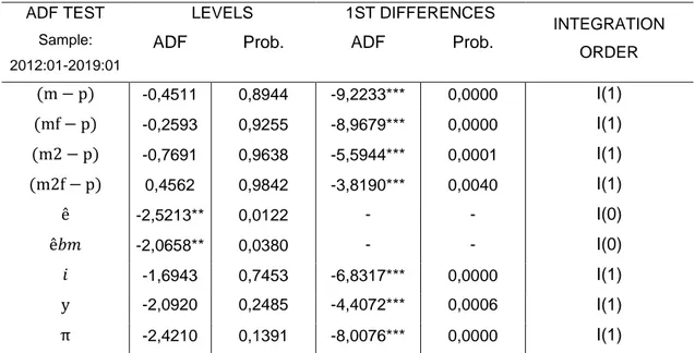
To verify the stationarity of the variables, the Augmented Dickey-Fuller (ADF) test was implemented to see how many times a variable must be differenced to obtain stationarity. Table 1 shows the ADF test statistics and the equivalent p-values.
Table 1 - Unit Roots Test
ADF TEST Sample: 2012:01-2019:01 LEVELS 1ST DIFFERENCES INTEGRATION ORDER
ADF Prob. ADF Prob.
(m − p) -0,4511 0,8944 -9,2233*** 0,0000 I(1) (mf − p) -0,2593 0,9255 -8,9679*** 0,0000 I(1) (m2 − p) -0,7691 0,9638 -5,5944*** 0,0001 I(1) (m2f − p) 0,4562 0,9842 -3,8190*** 0,0040 I(1) ê -2,5213** 0,0122 - - I(0) ê𝑏𝑚 -2,0658** 0,0380 - - I(0) 𝑖 -1,6943 0,7453 -6,8317*** 0,0000 I(1) y -2,0920 0,2485 -4,4072*** 0,0006 I(1) π -2,4210 0,1391 -8,0076*** 0,0000 I(1)
Notes: *, **, *** represents significance levels of 10%, 5% and 1%, respectively. In each test the lag length is decided according to the Akaike Information Criterion (AIC). I(0) represents stationary in levels and I(1) stationary in first differences. The test equation included trend and intercept for the interest rate and the real M2 (excluding FCD), none for both exchange rates and only intercept for the rest of the variables.
The results of the unit roots test suggest that all variables are stationary in first differences, except for both the exchange rates that are stationary in levels. Although both ê and êbm are I(0) the vector autoregressive (VAR) systems will include these variables to enrich the short-run dynamics.
12
3.4 Estimation Method
To examine the stability of domestic money demand and to check for presence of currency substitution, a cointegration analysis is performed using the Johansen (1988) Cointegration Test and the VECM for the estimation procedure. Alternative combinations of variables are applied.
Due to presence of I(1) variables in the money demand function, the appropriate methodology to follow is based on cointegration analysis. To start the empirical process, in each model an unrestricted VAR is estimated in the reduced form, where for each of the variables there is an equation, where the regressors in all equations are lagged values of the lagged variables (Stock & Watson, 2016). The number of lags is chosen considering the AIC.
Using an error correction term, there is a removal of trend and in this way the problems created by stochastic trends will be eliminated (Stock & Watson, 2016). If cointegration is found the VECM must be applied. A simple VECM specification, can be exhibited as the following one:
𝚫𝒚𝒕= 𝝈 + 𝚷𝒚𝒕−𝟏+ ∑𝑝−1𝑗=1𝚪𝒋𝚫𝒚𝒕−𝒋+ 𝝁𝒕,
where ∆𝒚𝒕 is the vector of dependent variables, 𝝈 are the intercepts,
𝚷 = 𝛂𝛃′, where 𝛂 is the matrix of adjustment coefficients, measuring the velocity at which
short-term deviations from the long-run relationship are reduced, and 𝜷 is the cointegration matrix, both are 𝑟 ∗ 𝐾 matrices, where 𝑟 is the number of cointegrating relations and 𝐾 is the number of
variables in the system, 𝑝 is the optimal number of lags, 𝑗 = 1, … , 𝑝 − 1, 𝝁𝒕 it’s a multivariate
white noise.
The simple ARDL model has as dependent variable the monthly inflation rate and the explanatory variables are given by the lagged monthly inflation rate and the excess liquidity. Afterwards, the price level forecast is performed where the ARDL is computed but only from January 2012 until January 2018 to, afterwards, forecast the models in a horizon of one year (February 2018 until January 2019).
4. Empirical Results
4.1 Cointegration Analysis
Tables 2 and 3 show the estimation results. To facilitate the analysis, the tables are divided according to each alternative dependent variable. Columns (1)-(3) have as dependent variable the real national monetary base, and the real broader monetary base results are exhibited in columns (4)-(6). In table 3, columns (7)-(9) represent the results when the dependent variable is the real narrow M2 and in columns (10)-(12) the dependent variable is the real broader M2. In each table, Panel 1 exhibits the results of the trace test of the Johansen Cointegration Test. In Panel 2, the results of the cointegrating equation (long-run model) are displayed (VECM results) and in Panel 3, results of the short-run coefficients of the cointegration equation are exhibited, but only, when the dependent variable is the money demand, since it is the main focus of the paper. Panel 4 shows the results of the serial correlation test.
In table 4 we display the likelihood-ratio (LR) test and the estimation results.
The maximum number of lags included was 6 and the optimal lags, according to the AIC, vary from 4 to 6 through all the systems. In table 2, the trace-test shows that there is at least one cointegrating relationship in each system, if a 10% significance level is considered. Columns (2), (3) and (6) stand out, given that they have more than one cointegrating relation, as opposite to the others. The same did not happen in table 3 in which two of the six systems did not exhibit a cointegrating relationship. Among them are the m2 − p, ê, i, y and m2f − p, ê, i, y. Both systems included the official depreciation of the exchange rate. Even though zero cointegration relationships were found, the VECM results for these systems were still computed, for
comparative purposes5.
Starting the analysis in table 2, a clear distinction is detected between the estimation results of the narrow money base and the broader money base. Both the estimations display relevant and statistically significant coefficients in columns (3) and (6), when the explanatory variables are just the interest rate and real income. This could lead to forejudge for a stable money demand, nevertheless, when the depreciation of the exchange rate is introduced these conclusion changes. In columns (1) and (2), both exchange rate depreciations exhibit negative and statistically significant coefficients at 5%, what is suggestive of currency substitution (Mizen & Pentecost, 1994). Nevertheless, in column (2) by including the black-market depreciation of exchange rate, the other outcomes are different from column (1): the interest rate, the real income and the adjustment coefficients are not statistically significant. What enhances the gap between the official and black-market exchange rates.
14 Table 2 - Johansen Cointegration Test and VECM results (part 1)
DEPENDENT VARIABLES NARROW MONETARY BASE, m − p BROAD MONETARY BASE, mf − p
SYSTEMS (1) (2) (3) (4) (5) (6)
EXPLANATORY VARIABLES ê, i, y êbm, i, y i, y ê, i, y êbm, i, y i, y
OBS. (after adjustments) 78 78 79 78 78 79
Lags (AIC) 6 6 6 6 6 6
PANEL 1 - Trace-test results
NONE 47,4721* 56,8797*** 38,5360*** 45,8383* 51,8936** 37,8084*** AT MOST 1 24,6939 28,4936* 16,7264** 22,9969 27,0169 13,6245* AT MOST 2 8,3751 6,7188 5,5439** 7,8690 6,8598 5,3784 AT MOST 3 1,9551 0,7539 1,7915 1,2573 NO. OF CE(S) 1 2 3 1 1 2 PANEL 2 - Long-run coefficients REAL MONEY (-1) -1,0000 -1,0000 -1,0000 -1,0000 -1,0000 -1,0000 Δ EXCHANGE RATE -4,9677** -3,7278** -2,4398 0,7101 (-2,0372) (-2,1457) (-0,9541) (0,6119) INTEREST RATE -2,5597** 1,4961 -7,9630*** -5,9594*** -5,8768*** -7,1171*** (-2,1066) (1,0949) (-4,23238) (-4,7422) (-6,2957) (-6,1920) REAL INCOME 4,2702*** 1,4235 7,2358*** 4,8875*** 4,4137*** 5,1297*** (3,1458) (0,8656) (3,2676) (3,6434) (3,8434) (3,7590) PANEL 3 - Adjustment coefficients D(REAL MONEY) 0,1779*** -0,0026 0,1158*** 0,1512*** 0,1614*** 0,1443*** (3,6449) (-0,0676) (4,2524) (3,8782) (3,8212) (4,4105) PANEL 4 – LM Test LRE*stat LM (2) 14,2304 11,7192 16,8603 15,3880 23,9210 14,6531 [0,5816] [0,7631] [0,0509] [0,4964] [0,0912] [0,1009] LM (6) 10,2781 10,7429 12,3081 9,7002 14,0009 11,0574 [0,8517] [0,8251] [0,1965] [0,8818] [0,5986] [0,2718]
Notes: *, **, ***: denote significance at 10%, 5% and 1%, respectively. T-statistics in () and p-value in []. Trace tests are evaluated with a constant in the cointegrating relation and in the error correction form. Real Money (-1) represents the real money with 1 lag. A restriction was imposed when estimating the VECM (the coefficient of the lagged dependent variable is equal to -1) to make it possible to read the signs of the coefficients directly. Own elaboration using EViews.
In columns (4) and (5) the coefficients of exchange rate depreciation are not statistically
significant, suggesting that currency substitution has no direct impact.In column (3) the number
of cointegrating relationships are excessive and the LM test shows that there is residuals serial correlation at 2 lags, suggesting a misspecification.
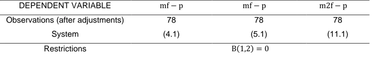
For robustness matters, to check if by using a broad monetary base the influence of this coefficient is eliminated, a restriction was imposed in columns (4) and (5) where exchange rate depreciation equals zero (in the long-run analysis). The results are displayed in columns (4.1) and (5.1) of table 4, and the conclusions remain the same: the effects of currency substitution cancel out when the real broader monetary base is used as dependent variable.
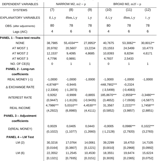
Table 3 - Johansen Cointegration Test and VECM results (part 2)
DEPENDENT VARIABLES NARROW M2, m2 − p BROAD M2, m2f − p
SYSTEMS (7) (8) (9) (10) (11) (12)
EXPLANATORY VARIABLES ê, i, y êbm, i, y i, y ê, i, y êbm, i, y i , y
OBS. (after adjustments) 80 78 78 80 78 78
Lags (AIC) 4 6 6 4 6 6
PANEL 1 - Trace-test results
NONE 38,7985 55,4334*** 27,8953* 40,7675 53,3062** 30,8012** AT MOST 1 20,9782 20,5607 13,2234 23,1553 24,5499 10,4773 AT MOST 2 12,1537 9,4095 4,8685 10,8393 8,8294 4,6171 AT MOST 3 4,7796 0,9891 4,7837 2,5433 NO. OF CE(S) 0 1 1 0 1 1 PANEL 2 - Long-run coefficients REAL MONEY (-1) -1,0000 -1,0000 -1,0000 -1,0000 -1,0000 -1,0000 Δ EXCHANGE RATE -4,8748** -0,9445 -448,7902*** -0,2324 (-2,3304) (-1,2873) (-3,5499) (-0,4083) INTEREST RATE 0,9262 -0,9999 -0,8855 185,8670*** -2,9559*** -3,3480*** (0,9447) (-1,6126) (-0,9435) (3,4652) (-7,0938) (-6,5877) REAL INCOME 4,7986*** 5,0310*** 4,4530*** 31,3567 2,2222*** 1,7458*** (4,2922) (6,8980) (4,4111) (0,5852) (3,9857) (2,8851) PANEL 3 – Adjustment coefficients D(REAL MONEY) 0,0029 0,0405 0,0443 -0,0005 0,0986*** 0,1022*** (0,1022) (1,1077) (1,2660) (-1,2128) (2,7920) (3,2783) PANEL 4 – LM Test LM (2) 30,3216 17,0764 14,0061 39,2299 18,4753 14,7105 [0,0164] [0,3807] [0,1221] [0,0010] [0,2968] [0,0992] LM (6) 22,3552 11,2545 10,4530 18,3551 19,6474 15,6224 [0,1321] [0,7935] [0,3151] [0,3035] [0,2365] [0,0752]
Notes: *, **, ***: denote significance at 10%, 5% and 1%, respectively. T-statistics in () and p-value in []. Trace tests are evaluated with a constant in the cointegrating relation and in the error correction form. Real Money (-1) represents the real money with 1 lag. A restriction was imposed when estimating the VECM (the coefficient of the lagged dependent variable is equal to -1) to make it possible to read the signs of the coefficients directly. Own elaboration using EViews.
16
It is important to have under consideration the two cases with no cointegrating relationship in table 3, for the reason that the results of the VECM estimation in both cases are odd: in column (7) the interest rate is not statistically significant and in column (10) the semi-elasticity of the interest rate is positive, and the real income is not statistically significant, what gives no trustable conclusions. Also, the loading factors do not exhibit statistically significance, pointing to the non-convergence of the real money balances to the equilibrium relationship. Hence, no further mention to these cases is made.
Comparing now the results of narrow M2 with the broader M2, once again, is clear the distinction between the estimation outcomes. First, no stable money demand equation is found when the dependent variable is the narrow M2 and the adjustment coefficients point to a non-convergence to the long-run relationship. The opposite happens when using the broader real M2. When the depreciation of the exchange rate is included in column (11) no statistically significant coefficient was found for this variable. When excluding the latter one from the system, column (12), a stable money demand is found where the semi-elasticity of the interest rate is negative, and the elasticity of real income is positive. In this situation, when we look to the LM test, both at 2 and 6 lags there is autocorrelation of the residuals if a 10% level is considered. So, since column (11) displays better results in the LM test, a restriction was imposed to the exchange rate depreciation coefficient in this column. From column (11.1), in table 4, we found a stable money demand for the broader M2 and there is no residual serial correlation. Leading us to conclude that even though depreciation of the exchange rate is not relevant in the long-run estimation, it should, at least, be included in the short-long-run system. According to the VEC
residuals heteroskedasticity tests (no cross terms)6, no heteroskedasticity was found.
Summing up, a pattern can be detected in here. The systems, that have as dependent variable the narrow real monetary aggregates, are more sensitive to the depreciation of the exchange rate, suggesting the presence of currency substitution and instability of domestic money demand. This goes according to Yildirim (2003), in which it is shown that when using a broader monetary aggregate, the domestic money demand function can become more reliable. Considering all said above, hypothesis 1 is confirmed.
The adjustment coefficients of short-run money demands are also reported in the tables. Since columns (2), (7), (8), (9) and (10) exhibit adjustment coefficients that are not statistically significant, pointing to a non-convergence of the real money balances to the equilibrium relationship, these systems are excluded from further analysis because no trustable conclusions could be taken if further computation was applied. System (3) is also excluded because it would
allow for omitted variable bias in further analysis.
Table 4 - Restrictions imposed to previous estimations
Notes: ***, **, *: denote significance at 1%, 5% and 10%, respectively. T-statistics in () and p-value in []. Trace tests are evaluated with a constant in the cointegrating relation and in the error correction form. Real Money (-1) represents the real money with 1 lag. A restriction was imposed when estimating the VECM (the coefficient of the lagged dependent variable is equal to -1) to make it possible to read the signs of the coefficients directly. Own elaboration using EViews.
4.2 ARDL estimation and inflation forecast
The fact that we identify stable money demand relationships with the expected coefficients does not necessarily imply that these systems contain useful information to forecast the price level. Based on this, in the current section the main purpose is to complement the previous analysis in order to verify if departures from the long-run relationship (excess liquidity) help to
predict the price level.7 In order to do so, an ARDL model is estimated for monthly inflation rate
experimenting with alternative excess liquidities as explanatory variables (from the previous estimations). Lag-lengths for each variable are automatically selected based on the AIC, that is
7 In the annex the excess liquidity (cointegrating relations) graphs can be found in figure 3.
DEPENDENT VARIABLE mf − p mf − p m2f − p
Observations (after adjustments) 78 78 78
System (4.1) (5.1) (11.1)
Restrictions B(1,2) = 0
LR test for binding restrictions (rank=1):
Chi-square (1) 0,5130 0,1523 0,0833 Probability 0,4739 0,6964 0,7729 REAL MONEY (-1) -1,0000 -1,0000 -1,0000 Δ EXCHANGE RATE 0,0000 0,0000 0,0000 INTEREST RATE -7,5692*** -5,6763*** -2,9453*** (-5,4566) (-5,9248) (-7,4976) REAL INCOME 5,6761*** 4,4512*** 2,1233*** (3,4943) (3,9022) (4,3536) Loading factors D(REAL MONEY) 0,1262*** 0,1504*** 0,1051*** (3,8672) (3,6006) (2,8358) Residual Tests LM (2) 16,8872 23,1835 18,0505 [0,3929] [0,1089] [0,3209] LM (6) 13,6529 14,0113 19,3324 [0,6246] [0,5979] [0,2518]
18
equal to 1 through all estimations. Table 5 summarizes the estimation results. Since all estimations exhibit heteroskedasticity, the Newey & West (1987) heteroskedastic consistent covariance estimator is used along with the ARDL estimation.
At a 10% significance level all excess liquidities are statistically significant in predicting inflation with exception of system (11.1). Nevertheless, only column (12) shows a 5% significance level for the coefficient on the excess liquidity (that corresponds to the estimates using the broader M2). This sustains the hypothesis enunciated in the beginning of this paper where broader monetary aggregates could have a better performance in forecasting inflation. No residual serial correlation was found.
For the tests on parameters stability, this study implemented the cumulative sum (CUSUM) and the cumulative sum of squares (CUSUMQ). If the plots stay within the 5 percent critical bound, it provides evidence that the parameters are stable. No breaks beyond the 5% level significance were found in the CUSUM test, but the same did not happen with the CUSUMQ, where all estimations exhibited a structural break.
Table 5 - ARDL estimation results of monthly inflation
Notes: ***, **, *: denote significance at 1%, 5% and 10%, respectively. T-statistics in parentheses. The “excess liquidity” was computed using the cointegrating vector (CIV) of the VECM estimations, where 𝐶𝐼𝑉 = 𝑟𝑒𝑎𝑙 𝑚𝑜𝑛𝑒𝑦 𝑏𝑎𝑙𝑎𝑛𝑐𝑒𝑠 − 𝑚𝑜𝑛𝑒𝑦 𝑑𝑒𝑚𝑎𝑛𝑑 𝑒𝑠𝑡𝑖𝑚𝑎𝑡𝑖𝑜𝑛𝑠. The lags were automatically selected using the AIC. Own elaboration using EViews.
DEPENDENT VARIABLE: MONTHLY INFLATION RATE
SYSTEMS (1) (4.1) (5.1) (6) (11.1) (12)
CIV (m − p) − md (mf − p) − md (m2f − p) − md
MONEY DEMAND (ê, i, y) (ê = 0, i, y) (êbm = 0, i, y) (i, y) (êbm = 0, i, y) (i, y)
SAMPLE 2012:01 – 2019:01
OBS. 84 84 84 84 84 84
INFLATION RATE (-1) 0,8184*** 0,7828*** 0,7918*** 0,7748*** 0,7933*** 0,7329*** (11,7709) (9,6158) (10,3539) (9,4686) (10,1963) (8,1281)
EXCESS LIQUIDITY (CIV)
0,003014* 0,0032* 0,0040* 0,0037* 0,0083 0,0120** (1,7404) (1,7997) (1,6912) (1,8528) (1,5879) (2,0514) CONSTANT (C) 0,0024*** 0,0029** 0,0028*** 0,0030*** 0,0028** 0,0036*** (2,6564) (2,6132) (2,6433) (2,6713) (2,5172) (2,7752) R2 0,7672 0,7700 0,7706 0,7716 0,7719 0,7817 S.E. REGRESSION 0,0043 0,0043 0,0043 0,0043 0,0043 0,0042 DURBIN WATSON 2,2332 2,1221 2,1460 2,1218 2,1549 2,1242 CUSUM 5% No break No break No break No break No break No break
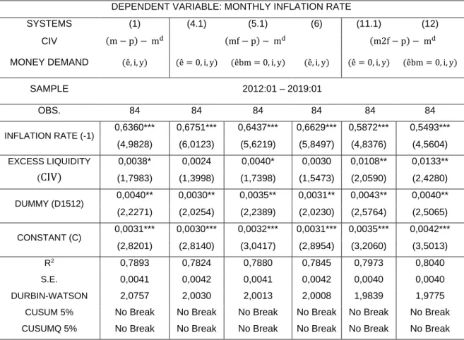
This structural break can be eliminated by creating a dummy (D1512) that assumes a value equal to 0 before December of 2015 and 1 until the end of the sample. The Chow Breakpoint Test was also computed for this specific structural break. The results are displayed in the annex (table 9).
When the dummy variable is included in the estimation procedure (table 6) the excess liquidity on system (11.1) becomes statistically significant at a 5% level and the excess liquidities of system (4.1) and (6) are now statistically insignificant. The coefficient of excess liquidity computed using the monetary aggregate M2 including FCD remains statistically significant at a 5% level and with a higher influence (0,0108 and 0,0133) than the excess liquidity computed using the national monetary base (0,0038).
Table 6 - ARDL estimation results when a dummy variable is included
DEPENDENT VARIABLE: MONTHLY INFLATION RATE
SYSTEMS (1) (4.1) (5.1) (6) (11.1) (12) CIV (m − p) − md (mf − p) − md (m2f − p) − md MONEY DEMAND (ê, i, y) (ê = 0, i, y) (êbm = 0, i, y) (ê, i, y) (ê = 0, i, y) (êbm = 0, i, y) SAMPLE 2012:01 – 2019:01 OBS. 84 84 84 84 84 84 INFLATION RATE (-1) 0,6360*** 0,6751*** 0,6437*** 0,6629*** 0,5872*** 0,5493*** (4,9828) (6,0123) (5,6219) (5,8497) (4,8376) (4,5604) EXCESS LIQUIDITY (CIV) 0,0038* 0,0024 0,0040* 0,0030 0,0108** 0,0133** (1,7983) (1,3998) (1,7398) (1,5473) (2,0590) (2,4280) DUMMY (D1512) 0,0040** 0,0030** 0,0035** 0,0031** 0,0043** 0,0040** (2,2271) (2,0254) (2,2389) (2,0230) (2,5764) (2,5065) CONSTANT (C) 0,0031*** 0,0030*** 0,0032*** 0,0031*** 0,0035*** 0,0042*** (2,8201) (2,8140) (3,0417) (2,8954) (3,2060) (3,5013) R2 0,7893 0,7824 0,7880 0,7845 0,7973 0,8040 S.E. 0,0041 0,0042 0,0041 0,0042 0,0040 0,0040 DURBIN-WATSON 2,0757 2,0030 2,0013 2,0008 1,9839 1,9775
CUSUM 5% No Break No Break No Break No Break No Break No Break
CUSUMQ 5% No Break No Break No Break No Break No Break No Break
Notes: ***, **, *: denote significance at 1%, 5% and 10%, respectively. T-statistics in parentheses. The “excess liquidity” was computed using the cointegrating vector (CIV) of the VECM estimations, where 𝐶𝐼𝑉 = 𝑟𝑒𝑎𝑙 𝑚𝑜𝑛𝑒𝑦 𝑏𝑎𝑙𝑎𝑛𝑐𝑒𝑠 − 𝑚𝑜𝑛𝑒𝑦 𝑑𝑒𝑚𝑎𝑛𝑑 𝑒𝑠𝑡𝑖𝑚𝑎𝑡𝑖𝑜𝑛𝑠. Own elaboration using EViews.
From these outcomes, the models that exhibited statistically significant coefficients were
estimated in a subsample (2012:02 – 2018:01)8. Afterwards, a forecast evaluation was made
20
for the price level (2018:02 – 2019:01)9. Both dynamic and static forecasts are examined to
allow for comparison.
The main purpose is to find out what is the monetary aggregate that best forecasts
inflation10. In order to do a more detailed analysis, this paper uses the root mean squared error
and the mean absolute error as in Dreger & Wolters (2014). And, for robustness, the Theil inequality coefficient is also considered. Lower values represent lower errors between the forecasted model and the actual model. The Theil inequality coefficient varies from 0 to 1, where 0 represents a perfect fit of both the forecasted model and the actual model. The purpose is to see which model has better forecasting ability.
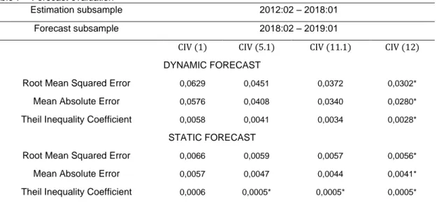
The results are displayed in table 7 where it is shown that not only CIV (12) exhibits the lower values compared to the other excess liquidities, but there is a clear conclusion that broader real money balances display a better performance in forecasting the price level, since CIV (5.1) and CIV (11.1) have lower values compared to CIV (1) as well. The
difference between the forecasted models using CIV (12) and using CIV (11.1) is not
significative, this would be expected since both use the broader M2 to calculate the excess liquidities. The static forecast has a better performance compared to the dynamic forecast, this happens because dynamic forecasting uses the forecasted value of the lagged dependent variable and static forecasting uses the actual value of the lagged dependent variable.
Table 7 – Forecast evaluation
Estimation subsample 2012:02 – 2018:01
Forecast subsample 2018:02 – 2019:01
CIV (1) CIV (5.1) CIV (11.1) CIV (12) DYNAMIC FORECAST
Root Mean Squared Error 0,0629 0,0451 0,0372 0,0302*
Mean Absolute Error 0,0576 0,0408 0,0340 0,0280*
Theil Inequality Coefficient 0,0058 0,0041 0,0034 0,0028*
STATIC FORECAST
Root Mean Squared Error 0,0066 0,0059 0,0057 0,0056*
Mean Absolute Error 0,0057 0,0047 0,0044 0,0041*
Theil Inequality Coefficient 0,0006 0,0005* 0,0005* 0,0005*
Notes: In each line the best performance is marked with *.
Broader monetary aggregates can predict in a better way the price level compared to narrow monetary aggregates. Having this, hypothesis 2 is also confirmed.
9 Using the ARDL forecast with EViews.
10The forecast is made using the ln(𝐶𝑃𝐼), based on the estimation results of [ln(𝐶𝑃𝐼
5. Conclusions
This study aims to find a stable domestic money demand in Angola using alternative monetary aggregates and, also, verifying the forecasting power of these monetary aggregates in predicting the inflation rate (from 2012:01 until 2019:01). Currency substitution is defined as the partial replacement of domestic currency by foreign currency in the basic functions of money, principally means of payment and store of value (Freitas & Veiga, 2006).
We identify a stable money demand for Angola when monetary aggregates contain FCD. This was verified in the long-run VECM estimation when using the narrow money base in which the coefficient of exchange rate depreciation was negative and statistically significant, which according to earlier studies gives an unstable money demand provided by the presence of currency substitution (Batten & Hafer, 1984; Calvo & Vegh, 1992; Cuddington, 1983; Mizen & Pentecost, 1994; Smith, 1995; Thomas, 1985). The opposite was observed when using the broader monetary aggregate M2, in which the depreciation of the exchange rate did not exhibit a statistically significant coefficient, hence, a stable money demand was found. Thus, the BNA, by using the national monetary base as the operational variable of the money targeting, is not taking into account the currency substitution phenomenon.
The fact that we identify stable money demand relationships with the expected coefficients does not necessarily imply that these systems contain useful information to forecast the price level, so using the excess liquidities of different models an ARDL estimation and a forecast evaluation was computed. Even though, none of the forecasts are perfectly fitted with the actual values, the better forecasting performance is from the broader M2.
When analysing and comparing this work with other studies it should be considered that there are some limitations in the data that can indeed change the results if more accurate data is provided by the BNA and other databases, in future years. Such limitations are that the CPI is from Luanda, instead as the whole country and the lack of data in the interest rate of treasury-bills. More data and more transparency are needed and to do so more studies in this country should be made. In future studies the expected depreciation of exchange rate should be used instead of the depreciation of exchange rate.
References
Angola Forex. (2019). Cotações do dia (BNA, Banca Comercial, Mercado Informal e Private Deals). Dezembro. Luanda.
Banco Nacional de Angola. (2014). Discurso do Governador do Banco Nacional de Angola, no encerramento do seminário sobre os desafios da desdolarização, Maio. Luanda.
Banco Nacional de Angola. (2017). Relatório de Estabilidade Financeira, Junho. Luanda.
Banco Nacional de Angola. (2018). Quadro Operacional para a Política Monetária, Junho. Luanda. Banco Nacional de Angola. (2019). Comité da Política Monetária, Novembro. Luanda.
Banco Nacional de Angola. (2020). Estatísticas Monetárias e Financeiras, nova série: Agregados Monetários. Março. Luanda.
Batten, D. S., & Hafer, R. W. (1984). Currency Substitution: A Test of Its Importance. Federal Reserve Bank of St. Louis, 5-12.
Bergstrand, J. H., & Bundt, T. P. (1990). Currency substitution and monetary autonomy: the foreign demand for US demand deposits. Journal of International Money and Finance, 9(3), 325–334. Branson, W. H., & Henderson, D. W. (1984). The Specification and Influence of Asset Markets.
Handbook of International Economics, 749-806.
Calvo, G., & Vegh, C. (1992). Currency Substituion in Developing Countries: An Introduction. IMF Working Paper 92/40, May. Washington: International Monetary Fund.
Chaisrisawatsuk, S., Sharma, S. C., & Chowdhury, A. R. (2004). Money demand stability under currency substitution: Some recent evidence. Applied Financial Economics, 14(1), 19–27. Cuddington, J. (1983). Currency Substitution, Capital Mobility and Money Demand. Journal of
International Money and Finance 2(2), 111-133.
Dalziel, P. (2002). The triumph of Keynes: What now for monetary policy research? Journal of Post
Keynesian Economics, 24(4), 511–527.
Dreger, C., & Wolters, J. (2010). M3 money demand and excess liquidity in the euro area. Public
Choice, 144(3), 459–472.
Dreger, C., & Wolters, J. (2014). Money Demand and the Role of Monetary Indicators in Forecasting Euro Area Inflation. International Journal of Forecasting 30, 303-312.
Federal Reserve Bank. (2018). Historical Approaches to Monetary Policy. March. Washington DC. Freitas, M., & Veiga, F. (2006). Currency Substitution, Portfolio diversification, and Money Demand.
Canadian Journal of Economics 39(3), 719–743.
Genc, I. H., Sahin, H., & Erol, T. (2005). Currency Substitution in Turkey. American Journal of Applied
Sciences 2(5), 920–925.
Giovanni, A., & Turtelboom, B. (1992). Currency Substitution. in F. van der Ploeg, ed., Handbook of
International Macroeconomics. Massachusetts: Blackwell.
Hossain, A. A. (2010). Monetary targeting for price stability in Bangladesh: How stable is its money demand function and the linkage between money supply growth and inflation? Journal of Asian
24 Instituto Nacional de Estatística. (2019). Produto Interno Bruto - I Trimestre de 2019, Nota de
Imprensa, July. Luanda.
Johansen, S. (1988). Statistical analysis of cointegration vectors. Journal of Economic Dynamics and
Control, 12(2–3), 231–254.
Mckinnon, R. (1982). Currency Substitution and Instability in the World Dollar Standard. The
American Economic Review, 72(3), 320–333.
Miles, M. A. (1978). Currency Substition, Flexible Exchange Rates, and Monetary Independence.
American Economic Review, 68(3), 428–436.
Miles, M. A. (1981). Currency Substitution: Some Further Results and Conclusions. Southern
Economic Association, 48(1), 78–86.
Mizen, P., & Pentecost, E. (1994). Evaluating the Empirical Evidence for Currency Substitution: A Case Study of the Demand for Sterling in Europe. The Economic Journal, 104(426), 1057– 1069.
Newey, W., & West, K. (1987). Hypothesis Testing with Efficient Method of Moments Estimation.
International Economic Review, 28(3), 777–787.
Owoye, O., & Onafowora, O. (2007). M2 Targeting, Money Demand, and Real GDP Growth in Nigeria: Do Rules Apply? Journal of Business and Public Affairs, 1(2), 1–20.
Prock, J., Soydemir, G. A., & Abugri, B. A. (2003). Currency substitution: Evidence from Latin America. Journal of Policy Modeling, 25(4), 415–430.
Samuelson, P., & Nordhaus, W. (2010). Economics, 19th Edition. New York: McGraw-Hill
Companies.
Smith, C. E. (1995). Substitution, Income, and Intertemporal Effects In Currency‐Substitution Models.
Review of International Economics, 3(1), 53–59.
Stock, J., & Watson, M. (2016). Introduction to Econometrics. Harlow: Person Education Limited. Thomas, L. R. (1985). Portfolio Theory and Currency Substitution. Journal of Money, Credit and
Banking, 17(3), 347–357.
Végh, C. A. (1989). The optimal inflation tax in the presence of currency substitution. Journal of
Monetary Economics, 24(1), 139–146.
Yildirim, J. (2003). Currency Substitution and the Demand for Money in Five European Union Countries. Journal of Applied Economics, 6(2), 361–383.
Zervoyianni, A. (1992). International macroeconomic interdependence, currency substitution, and price stickiness. Journal of Macroeconomics, 14(1), 59–86.
Annex
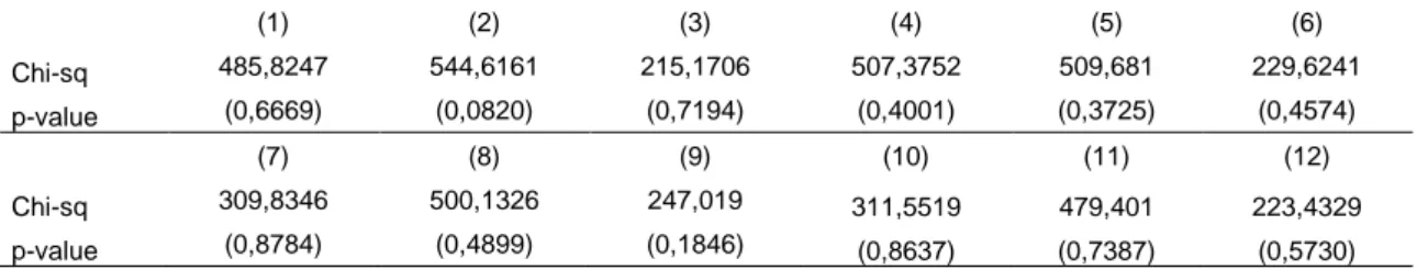
Table 8 - VECM Heteroskedasticity test
VEC Residual Heteroskedasticity Test
(1) (2) (3) (4) (5) (6) Chi-sq 485,8247 544,6161 215,1706 507,3752 509,681 229,6241 p-value (0,6669) (0,0820) (0,7194) (0,4001) (0,3725) (0,4574) (7) (8) (9) (10) (11) (12) Chi-sq 309,8346 500,1326 247,019 311,5519 479,401 223,4329 p-value (0,8784) (0,4899) (0,1846) (0,8637) (0,7387) (0,5730)
VEC Residual Heteroskedasticity Test (Restrictions)
(4.1) (5.1) (11.1)
Chi-sq 508,4098 504,2668 477,6921
p-value (0,3876) (0,4382) (0,7565)
Table 9 - Chow Breakpoint Test
Chow Breakpoint Test: 2015M12 Equation sample: 2012M02 2019M01
CIV F-statistic Prob. F (3,78) Log likelihood ratio Prob. Chi-Square (3)
(1) 3,6024 (0,0171) 10,8998 (0,0123) (4.1) 3,1158 (0,0309) 9,5076 (0,0233) (5.1) 4,2741 (0,0076) 12,7843 (0,0051) (6) 3,3301 (0,0238) 10,1235 (0,0175) (11.1) 7,5002 (0,0002) 21,2901 (0,0001) (12) 6,8496 (0,0004) 19,6428 (0,0002)
Notes: Chow Breakpoint test at the specified breakpoint in each monthly inflation equation using different excess liquidities. Own elaboration using EViews.
Table 10 - ARDL estimation results (small sample) for forecasting purposes
DEPENDENT VARIABLE: MONTHLY INFLATION RATE
SYSTEMS (1) (4.1) (5.1) (6) (11.1) (12) CIV (m − p) − md (mf − p) − md (m2f − p) − md MONEY DEMAND (ê, i, y) (ê = 0, i, y) (êbm = 0, i, y) (ê, i, y) (ê = 0, i, y) (êbm = 0, i, y) SAMPLE 2012M02 - 2018M01 OBS. 72 72 72 72 72 72 INFLATION RATE (-1) 0,5369 0,6501 0,6217 0,6396 0,5774 0,5467 (4,3392) (6,0575) (5,6140) (5,8747) (4,6846) (4,3918) EXCESS LIQUIDITY (CIV) 0,0052 0,0022 0,0039 0,0028 0,0102 0,0130 (2,2408) (1,2509) (1,5254) (1,3743) (1,7100) (2,0157) DUMMY (D1512) 0,0062 0,0043 0,0046 0,0043 0,0052 0,0046 (3,2987) (2,4918) (2,6996) (2,4832) (2,9481) (2,8203) CONSTANT (C) 0,0039 0,0031 0,0033 0,0032 0,0036 0,0042 (3,5328) (2,9399) (3,1279) (2,9735) (3,1324) (3,2170) R2 0,8525 0,8388 0,8430 0,8403 0,8499 0,8551 S.E. OF THE REGRESSION 0,0037 0,0038 0,0038 0,0038 0,0037 0,0036 DURBIN-WATSON 1,9064 1,7841 1,7993 1,7872 1,7830 1,7875
CUSUM 5% No Break No Break No Break No Break No Break No Break
CUSUMQ 5% No Break No Break No Break No Break No Break No Break
Notes: *, **, ***: denote significance at 10%, 5% and 1%, respectively. T-statistics in parentheses. The “excess liquidity” was computed using the cointegrating vector (civ) of the VECM estimations, where 𝐶𝐼𝑉 = 𝑟𝑒𝑎𝑙 𝑚𝑜𝑛𝑒𝑦 𝑏𝑎𝑙𝑎𝑛𝑐𝑒𝑠 − 𝑚𝑜𝑛𝑒𝑦 𝑑𝑒𝑚𝑎𝑛𝑑 𝑒𝑠𝑡𝑖𝑚𝑎𝑡𝑖𝑜𝑛𝑠. The lags were automatically selected using the AIC. Own elaboration using EViews.
26 Figure 3 - Cointegration graphs
-0.8 -0.4 0.0 0.4 0.8 1.2 2012 2013 2014 2015 2016 2017 2018 CIV (1) -1.2 -0.8 -0.4 0.0 0.4 0.8 2012 2013 2014 2015 2016 2017 2018 CIV (4.1) -.8 -.4 .0 .4 .8 2012 2013 2014 2015 2016 2017 2018 CIV (5.1) -1.2 -0.8 -0.4 0.0 0.4 0.8 2012 2013 2014 2015 2016 2017 2018 CIV (6) -.3 -.2 -.1 .0 .1 .2 .3 .4 2012 2013 2014 2015 2016 2017 2018 CIV (11.1) -.3 -.2 -.1 .0 .1 .2 .3 .4 2012 2013 2014 2015 2016 2017 2018 CIV (12)