2018
UNIVERSIDADE DE LISBOA
FACULDADE DE CIÊNCIAS
DEPARTAMENTO DE BIOLOGIA VEGETAL
Extracting Biomedical Relations from Biomedical
Literature
Tânia Sofia Guerreiro Maldonado
Mestrado em Bioinformática e Biologia Computacional
Especialização em Bioinformática
Dissertação orientada por:
Resumo
A ciência, e em especial o ramo biomédico, testemunham hoje um crescimento de conhecimento a uma taxa que clínicos, cientistas e investigadores têm dificuldade em acompanhar. Factos científicos espalhados por diferentes tipos de publicações, a riqueza de menções etiológicas, mecanismos moleculares, pontos anatómicos e outras terminologias biomédicas que não se encontram uniformes ao longo das várias publicações, para além de outros constrangimentos, encorajaram a aplicação de métodos de text mining ao processo de revisão sistemática.
Este trabalho pretende testar o impacto positivo que as ferramentas de text mining juntamente com vocabulários controlados (enquanto forma de organização de conhecimento, para auxílio num posterior momento de recolha de informação) têm no processo de revisão sistemática, através de um sistema capaz de criar um modelo de classificação cujo treino é baseado num vocabulário controlado (MeSH), que pode ser aplicado a uma panóplia de literatura biomédica.
Para esse propósito, este projeto divide-se em duas tarefas distintas: a criação de um sistema, constituído por uma ferramenta que pesquisa a base de dados PubMed por artigos científicos e os grava de acordo com etiquetas pré-definidas, e outra ferramenta que classifica um conjunto de artigos; e a análise dos resultados obtidos pelo sistema criado, quando aplicado a dois casos práticos diferentes.
O sistema foi avaliado através de uma série de testes, com recurso a datasets cuja classificação era conhecida, permitindo a confirmação dos resultados obtidos. Posteriormente, o sistema foi testado com recurso a dois datasets independentes, manualmente curados por investigadores cuja área de investigação se relaciona com os dados. Esta forma de avaliação atingiu, por exemplo, resultados de precisão cujos valores oscilam entre os 68% e os 81%.
Os resultados obtidos dão ênfase ao uso das tecnologias e ferramentas de text mining em conjunto com vocabulários controlados, como é o caso do MeSH, como forma de criação de pesquisas mais complexas e dinâmicas que permitam melhorar os resultados de problemas de classificação, como são aqueles que este trabalho retrata.
Palavras-chave: prospeção de texto, vocabulários controlados, literatura biomédica, MeSH,
Abstract
Science, and the biomedical field especially, is witnessing a growth in knowledge at a rate at which clinicians and researchers struggle to keep up with. Scientific evidence spread across multiple types of scientific publications, the richness of mentions of etiology, molecular mechanisms, anatomical sites, as well as other biomedical terminology that is not uniform across different writings, among other constraints, have encouraged the application of text mining methods in the systematic reviewing process.
This work aims to test the positive impact that text mining tools together with controlled vocabularies (as a way of organizing knowledge to aid, at a later time, to collect information) have on the systematic reviewing process, through a system capable of creating a classification model which training is based on a controlled vocabulary (MeSH) that can be applied to a variety of biomedical literature.
For that purpose, this project was divided into two distinct tasks: the creation a system, consisting of a tool that searches the PubMed search engine for scientific articles and saves them according to pre-defined labels, and another tool that classifies a set of articles; and the analysis of the results obtained by the created system when applied to two different practical cases.
The system was evaluated through a series of tests, using datasets whose classification results were previously known, allowing the confirmation of the obtained results. Afterwards, the system was tested by using two independently-created datasets which were manually curated by researchers working in the field of study. This last form of evaluation achieved, for example, precision scores as low as 68%, and as high as 81%.
The results obtained emphasize the use of text mining tools, along with controlled vocabularies, such as MeSH, as a way to create more complex and comprehensive queries to improve the performance scores of classification problems, with which the theme of this work relates.
Keywords: text mining, systematic review, controlled vocabularies, biomedical literature, MeSH,
Acknowledgments
To Prof. Dr. Francisco Couto, my advisor, for the guidance and wise words along this path.
To FCT and LASIGE, for support through funding of the Programa Estratégico da Unidade de
I&D LASIGE – Laboratório de Sistemas Informáticos de Grande-Escala project, with ref.
UID/CEC/00408/2013.
To André Lamúrias, whose help was fundamental when anything else seemed to fail.
To Melinda Noronha, Jenni Moore, and Jan Nordvik, for the kindly provided data and the different perspectives provided to the project.
Last but not least, to my family. For all the support along these years, through rough times and moments of joy, and for making me who I am today.
“Para ser grande, sê inteiro: nada Teu exagera ou exclui.
Sê todo em cada coisa. Põe quanto és No mínimo que fazes.”
Ricardo Reis, in "Odes" Heteronym of Fernando Pessoa
Index
List of Figures ... ix
List of Tables ... x
List of Acronyms ... xi
Section 1 Introduction ... 1
Problem ... 1
Objectives ... 2
Results ... 3
Contributions ... 3
Document Structure ... 3
Section 2 Concepts and Related Work ... 4
2.1.
Systematic Reviews ... 4
2.2.
Text Mining ... 5
2.2.1.
Information Retrieval ... 5
2.2.1.1. Natural Language Processing Techniques ... 6
Sentence Splitting ... 6
Tokenization ... 6
Stemming & Lemmatization ... 7
Machine Learning... 7
2.2.1.2. Performance Assessment ... 12
2.2.1.3. Cross-Validation ... 14
2.3.
Controlled Vocabularies ... 15
2.3.1.
Medical Subject Headings (MeSH) ... 16
2.3.1.1. MeSH Structure ... 16
2.3.1.2. Online Retrieval with MeSH ... 17
2.3.1.3. Example ... 18
2.4.
Text Mining within Systematic Reviews ... 18
2.5.
Related Tools ... 19
2.6.
Resources ... 21
2.6.1.
Biopython ... 21
2.6.2.
NLTK ... 22
2.6.3.
Scikit-learn ... 22
2.6.3.1. Vectorization ... 23
2.6.3.2. Cross-Validation ... 23
2.6.3.3. Classification ... 24
Multinomial Naïve Bayes ... 24
K-Nearest Neighbors ... 24
Decision Tree ... 24
Random Forest ... 24
Logistic Regression ... 25
Multi-Class Classification ... 25
Grid Search ... 25
2.6.3.4. Performance Analysis ... 26
2.6.3.5. Model Evaluation ... 27
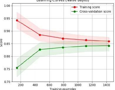
Learning Curve ... 27
ROC Curve ... 27
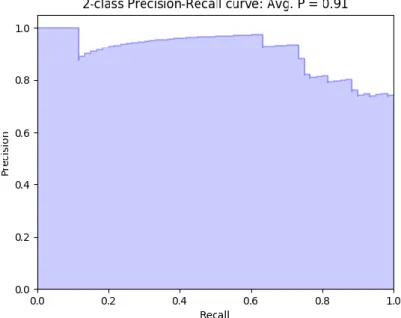
PR Curve ... 28
Section 3 Developed Work... 29
3.1.
Methodology ... 29
3.2.
Overview ... 29
3.3.
Script Development ... 30
3.3.1.
PubMed Search & Save ... 30
3.3.2.
Classifier... 31
3.3.2.1.
Model Evaluation ... 33
3.4.
Datasets ... 33
3.4.1.
Mindfulness/Fatigue ... 34
3.4.2.
Humanin ... 35
3.4.
Practical Applications ... 35
3.5.1.
Mindfulness/Fatigue Dataset ... 35
3.5.2.
Humanin Dataset ... 37
Section 4 Results & Discussion ... 40
4.1.
Results ... 40
4.1.1.
Mindfulness/Fatigue Dataset ... 40
4.1.1.1.
Model Evaluation ... 41
4.1.2.
Humanin Dataset ... 43
4.1.2.1.
Model Evaluation ... 45
4.2.
Discussion ... 47
Section 5 Conclusions & Future Work ... 51
5.1.
Summary ... 51
5.1.1.
Limitations ... 51
Bibliography ... 54
Annex ... 59
A.
ROC Curve Example ... 59
B.
MeSH Browser Search Example ... 59
C. Model Evaluation – Bag of Words ... 60
D. Model Evaluation – Confusion Matrix ... 60
E.
Humanin Article List ... 61
F.
Practical Applications – Mindfulness Dataset Classification Reports ... 64
List of Figures
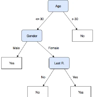
Figure 2.1 - Decision tree presenting response to direct mailing (adapted from [30]) ... 10
Figure 2.2 - Diagram for comprehension of precision and recall concepts ... 13
Figure 2.3 - MeSH hierarchy tree for "brain" term ... 18
Figure 2.4 - Classification report output example ... 26
Figure 2.5 - Example of learning curve using Naïve Bayes classifier ... 27
Figure 2.6 - Example of ROC curve ... 28
Figure 2.7 - Example of precision-recall curve with average precision of 0.91 ... 28
Figure 3.1 - Proposed methodology………..30
Figure 3.2 - Proposed pipeline………...30
Figure 3.3 - “PubMed Search and Save” example run ... 31
Figure 3.4 - "Classifier" script example run ... 32
Figure 3.5 - Search process and study selection flowchart (adapted from [71]) ... 34
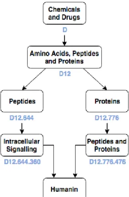
Figure 3.6 - Humanin MeSH hierarchy tree ... 38
Figure 4.1 - Learning curves for the "train" training set and logistic regression classification algorithm ... 42
Figure 4.2 - ROC curve for the "train" training set and logistic regression classification algorithm ... 42
Figure 4.3 – Precision-recall curve for the "train" training set and logistic regression classification algorithm ... 43
Figure 4.4 - Learning curves for the "train 4" training set and logistic regression classification algorithm ... 46
Figure 4.5 - ROC curve for the "train 4" training set and logistic regression classification algorithm ... 46
Figure 4.6 - Precision/recall curve for the "train 4" training set and logistic regression classification algorithm ... 47
Figure 1 - Example and explanation of a ROC curve (adapted from [72])……….………..59
Figure 2 - MeSH browser example, using the search term "brain"………60
Figure 3 - Bag of words and TF-IDF score for each word and label……….60
List of Tables
Table 2.1 - Confusion matrix with evaluation measures………..13
Table 3.1 - Queries for the mindfulness training set article retrieval………….………36
Table 3.2 - Queries for the Humanin training set article retrieval………38
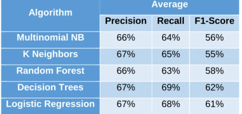
Table 4.1 - Average score of all classification trials with the mindfulness dataset……….40
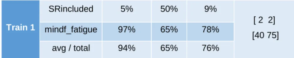
Table 4.2 - Classification reports for "train" and "train 1", using the Random Forest algorithm….40 Table 4.3 - Classification report for "train 3", using the Random Forest algorithm………...41
Table 4.4 - Average score of all classification trials with the humanin dataset……….44
Table 4.5 - Classification reports for "train 4" and "train 5”, using the Logistic Regression algorithm………...44
Table 4.6 - Classification report for "train 2", using the K-Neighbors algorithm………45
Table 4.7 - Queries for the "SRincluded" class from the Mindfulness/fatigue dataset……….…..48
Table 4.8 - MeSH terms for the "train 3" PubMed queries……….48
Table 4.9 - Queries for the "relevant" class from the Humanin dataset………..49
Table 1 - Humanin article list and corresponding classification……….61
Table 2 - Classification report for the mindfulness dataset, for each training set and algorithm..64
List of Acronyms
API Application Programming Interface
AUROC Area Under the Receiver Operator Characteristic
CS Citation Screening
CV Cross Validation
EL Entity Linking
FDA Food and Drug Administration
FN False Negative
FP False Positive
FPR False Positive Rate
IDF Inverse Document Frequency
IM Index Medicus
IR Information Retrieval
k-NN k-Nearest Neighbors
MAP Maximum A Posteriori
MeSH Medical Subject Headings
ML Machine Learning
NCBI National Center for Biotechnology Information
NER Named Entity Recognition
NLP Natural Language Processing
NLTK Natural Language Toolkit
PICOS Participants, Interventions, Comparators, Outcomes and Study design
PR Precision-Recall
RE Relation Extraction
ROC Receiver Operator Characteristic
SCR Supplementary Chemical Records
SR Systematic Review
SVC Support Vector Classification
SVM Support Vector Machines
TBS Token Boundary Symbol
TF Term Frequency
TF-IDF Term Frequency-Inverse Document Frequency
TM Text Mining
TN True Negative
TP True Positive
Section 1
Introduction
Science is currently witnessing the fast pace at which knowledge grows, especially in the biomedical field.
One of the first organizations to index medical literature was the US National Library of Medicine (NLM), in 1879: the Index Medicus (IM) was a comprehensive bibliographic index of life science and biomedical science information, that would in 1996 become the MEDLINE database.
The US Food and Drug Administration (FDA) introduced in 1962 a regulatory framework that required proof of the efficiency of new drugs [1], and other countries followed the practice. This led to an inevitable rise in the number of randomized controlled trials (i.e., a study in which the participants are assigned by chance to separate groups, according to the National Cancer Institute), and at the same time, the overall rise in the number of scientific articles, many providing evidence base for these trials. In 1966, the NLM had indexed 165,255 articles for Index Medicus; in 1985, the number of articles was 73% higher, with a total of 286,469 articles indexed [2]. By 2006, the index had grown to nearly 10 million references [3] that would cover areas such as medicine, nursing, pharmacy, dentistry, veterinary medicine, and healthcare. As of 2017, PubMed (a search engine that primarily accesses the MEDLINE database) contains more than 27 million citations for biomedical literature.
As the number of clinical trials raised, so did the science of reviewing trials, which aim to make sense of multiple studies. According to Bastian [3], there are now 75 new trials and 11 new systematic reviews (SR) of trials per day, haven’t yet reached a plateau in growth.
Clinicians and researchers are required to keep up with published scientific studies and use them in their field of work. However, with the massive amount of data that the all-new high-throughput molecular biology techniques and studies now produce, as well as the increasingly widespread adoption of health information systems that store clinical data, evidence-based science is increasingly becoming a more laborious task.
Problem
Finding the best scientific evidence that applies to a given problem is becoming exceedingly difficult due to the exponential growth of biomedical publications, which considers several types of publications such as:
(i) scientific publications, (ii) patents,
(iv) a plethora of regulatory, market, financial, and patent intelligence tools.
Scientific journals, the type of publication most widely used, tend to share a general arrangement (Title, Abstract, Introduction, Materials and Methods, Experiments, Results, Discussion, and Summary and Conclusion sections) although with considerable variability across publishers and themes.
Another obstacle lies in the fact that biomedical literature is plentiful in mentions of etiology, molecular mechanisms, clinical conditions, anatomical sites, medications, and procedures. Even though the language used for scientific discussion is formal, the names of the biomedical entities may not be uniform across different writings.
This plenitude of different terminologies motivates the application of text mining (TM) methods to enable efficient indexing and determination of similarities between the search terms in a given search engine and the retrieved document. Nonetheless, TM has been applied successfully to biomedical documents, for example, to identify protein-protein interactions [4] and associations between drugs [5].
More than recognizing entities within a given set of documents, it is crucial to recognize the search terms as a biomedical term (or set of terms) during the SR process, providing researchers with better tools to systematic review the existing literature. A common strategy involves linking text to a controlled vocabulary.
Objectives
The main objective of this work is to test the hypothesis that TM tools and controlled vocabularies have a positive impact on the systematic reviewing process, either from an aspect of time reduction or regarding performance (i.e., if a given article is relevant to the study or not).
For the accomplishment of this objective, it will be developed a system capable of creating a classification model which training is based on a controlled vocabulary (Medical Subject Headings – MeSH) that can be applied on a variety of biomedical literature.
This will optimistically provide researchers with a semi-automated systematic reviewing tool that aids them in keeping up with scientific studies, regarding the amount of time saved in research, as well as providing better support for decision-making.
The work described in this dissertation comprises two distinct tasks:
(i) the creation of a system consisting of a tool that searches the PubMed search engine for scientific articles and saves them according to pre-defined labels, and another tool that classifies a set of articles;
(ii) the analysis of the results obtained by the created system when applied to two different practical cases.
Results
The system was evaluated initially through a series of tests, using datasets whose classification results were previously known, allowing the confirmation of the obtained results. Afterwards, the system was tested by using two independently-created datasets which were manually curated by researchers working in the field of study. This last form of evaluation achieved, for example, precision scores as low as 68%, and as high as 81% (average score between two classes, on the Humanin dataset), depending on the controlled vocabulary terms used to train the system.
Contributions
The main contribution of this work is a system capable of creating a classification model in which training is based on a controlled vocabulary (MeSH) that can be applied to a variety of biomedical literature1.
Document Structure
The following sections are organized as follows:
Section 2 focuses on all the work done by third-party entities, i.e., it explains the main concepts applied in this research, presents an overview of the state-of-the-art tools in the area, and showcases the resources that will be further applied;
Section 3 presents all the work developed for this thesis, including the system developed, the methodology followed and the datasets used;
Section 4 demonstrates the results achieved in each study case, and ends with a discussion of all the results obtained;
Section 5 presents the conclusions achieved by this work, its limitations, some suggestions for future work, and finishes with some final remarks.
Section 2
Concepts and Related Work
This section is dedicated to describing some concepts necessary to contextualize this project, namely a description of systematic reviews, text mining, and controlled vocabularies, as well as presenting some related work.
2.1. Systematic Reviews
Systematic reviews were invented as a means to enable clinicians to use evidence-based medicine, to support clinical decisions [6]. SR identify, assess, synthesize, and interpret multiple published and unpublished studies in a given topic, improving decision-making for a variety of stakeholders [7], while also allow identifying research challenges to develop new research ideas.
The systematic reviewing process is conducted through a robust but slow and human-intensive process. According to Jonnalagadda et al. [8], a SR process includes seven steps:
1. Definition of the review question and development of criteria for including studies; 2. Search for studies addressing the review question;
3. Selection of studies that meet the criteria for inclusion in the review – citation screening (CS);
4. Extraction of data from included studies;
5. Assessment of the risk of bias in the included studies, by appraising them critically; 6. Where appropriate, an analysis of the included data by undertaking meta-analyses should be made;
7. Address reporting biases.
For reviews to be systematic, the search task has to ensure relevant literature is retrieved as much as possible, even at the cost of retrieving up to tens of thousands of irrelevant documents. It also involves searching multiple databases. Therefore, reviewers require specific knowledge of dozens of literary and non-literary databases, each with its own search engine, metadata, and vocabulary [6].
Given the amount of time it takes to filter out the immense quantity of research that will not be covered, a SR can take a considerable amount of time to complete. This is often a problem, since decision-making needs to happen quite fast, and there is not always the opportunity for a review to be concluded, even if it leads to a better decision.
There are several possible ways to reduce screening workload. As suggested by O'Mara-Eves et al. [9], these may be summed as follows:
reducing the number of items that need to be screened manually; reducing the number of experts needed to screen the items;
increasing the rate (or speed) of screening; improving the workflow.
To reduce the workload, there are ongoing efforts to automate part or all of the stages of the SR process. One approach is the application of Machine Learning (ML) techniques using TM to automate the CS (also called study selection) stage. Since the ML prediction performance is generally on the same level as the human prediction performance, using a ML-based system will lead to significant workload reduction for the human experts involved in the systematic review process [9].
2.2. Text Mining
Tan [10] described TM as “the process of extracting interesting and non-trivial patterns or knowledge from unstructured text documents.” According to Hotho [11], TM is a multi-disciplinary field in computer science that relies on information retrieval, machine learning, statistics, computational language, and data mining.
Research in this area is still in a state of significant flux, indicated by the sometimes confusing use of terms. Hotho et al. [11], for instance, presented different TM definitions, driven by the specific perspective of the area. The first approach considered that TM essentially corresponds to information retrieval (IR); a second strategy referred to TM as the application of algorithms and methods from machine learning and statistics to texts, aiming to find useful patterns.
Regarding biomedical TM, to name a few of the most typical tasks, one can point out: Information Retrieval (IR): to rank or classify articles for topics of relevance,
Named Entity Recognition (NER): detect a variety of different types of bioentity mentions, Entity Linking (EL): index or link documents to terms from controlled vocabularies or
bio-ontologies, and
Relations Extraction (RE): extract binary relationships between bioentities, in particular, protein or gene relations, like protein−protein interactions.
Despite the differences in focus and scope of the several biomedical branches, end users have mutual information demands: from finding papers of relevance (IR) to the assignment of predefined classes to text documents (formally known as classification).
The tasks of TM on which this work mainly focuses on are IR and classification, and therefore those will be described in the next sub-sections. A small description of other tasks, not addressed in this work but also relevant to the biomedical domain, will also be presented.
2.2.1. Information Retrieval
information retrieval was later used for the first time by Calvin Mooers, in 1950 [12].
As defined by Manning et al. [12] “IR is finding material (usually documents) of an unstructured nature (usually text) that satisfies an information need from within large collections (usually stored on computers).” The term “unstructured” mentions data that does not have clear, semantically explicit structure, that is easy for a computer to understand. It is the opposite of structured data, which the better example is a relational database.
In other words, IR is a task of TM that deals with automatically finding relevant texts from large datasets of unstructured text, where manual methods would typically be infeasible [13].
2.2.1.1.
Natural Language Processing Techniques
In most of the cases, the information demand concerns human language texts. Natural language processing (NLP) deals with the interactions between computers and human (natural) languages, particularly, with parsing the input text into a machine-readable form.
The following NLP techniques are some of the most commonly used in text mining systems, and they are also broadly applied in the biomedical domain:
Sentence Splitting
A low-level text processing step that consists of separating written text into individual sentences [14]. Follows simple heuristic rules, for example, a space followed by a capital letter should be separated [15]. Some exceptions could be “Dr. Xxx” or “e.g., YYY.”
Tokenization
Given a character sequence and a defined document unit, tokenization is the task of cutting it into smaller pieces, called tokens [12]. It is usually the first step in a text processing system, and if wrongly implemented, can lead to a poor-performing system [16].
Although these tokens are usually related to single words, they may also consist of numbers, symbols or even phrases. It has been observed that in biomedical documents, symbols that usually correspond to token boundary symbols (TBS), such as “+,” “/” and “%,” do not always denote correct boundary elements.
A tokenization parser is used to retrieve these tokens from the text, splitting the input based on a set of predefined rules. The output of various tokenizers can be significantly different, for instance, depending on how characters such as hyphens are handled [14], [17]. Two examples of systems
developed specially for text written in the English language are the Stanford Tokenizer2 and
Banner3.
Stemming & Lemmatization
The tokens are usually normalized before being added to a given term list; that is, a linguistic pre-processing step is carried out to generate a modified token representing the canonical form of the corresponding term [14]. Typically, this step refers to either stemming or lemmatization. Both aim to reduce words to their common base form: for instance, “am,” “are” and “is” would become “be”; “car,” “cars,” “car’s” and “cars” would become “car.”
The difference between both techniques is that stemming usually refers to a heuristic process that slices the ends of words, hoping to achieve this goal correctly most of the time. Lemmatization, on the other hand, attempts to perform a vocabulary correctly and morphological analysis of words, typically aiming to remove inflectional endings only and to return the dictionary form of a word (known as the lemma). However, to achieve this, the word form must be known, i.e., the part of speech of every word in the text document has to be assigned. Since this tagging process is usually very time-consuming and error-prone, stemming methods are applied alternatively [11].
Porter’s stemming algorithm4 has been shown to be empirically very effective [12]. It is a process
for removing the commoner morphological and inflexional endings from words in English [18].
The BioLemmatizer5 is a domain-specific lemmatization tool for the morphological analysis of
biomedical literature, achieving very high-performance scores when evaluated against a gold standard of manually labeled biomedical full-text articles [14], [19].
Machine Learning
One approach that has increasingly become the method of choice for many text classification tasks is Machine Learning. ML is a field of computer science which applies statistical techniques so that computer systems can "learn" (i.e., progressively improving its performance on a specific task) with data, without being explicitly programmed for it [20].
Regarding the classification problem, and given a set of classes, the user seeks to determine which class(es) a given document belongs to. More formally, the classification problem is defined
2 https://nlp.stanford.edu/software/tokenizer.shtml
3 https://github.com/oaqa/banner/blob/master/src/main/java/banner/tokenization/Tokenizer.java 4 https://tartarus.org/martin/PorterStemmer/index.html
as follows: having a training set 𝐷⟨𝑑𝑖⟩, 𝑖 = 1,2, … , 𝑛 of documents, such that each document 𝑑𝑖 is labeled with a label 𝐶 = {𝑐1, 𝑐2, … , 𝑐𝑗}, the task is to find a classification model (a classifier) 𝑓 where
𝑓: 𝐷 → 𝐶𝑓(𝑑) = 𝑐 (2.1)
Which can assign the correct class label to a new document 𝑑 (test instance) [21].
There are two main ML categories: supervised, and unsupervised learning. For supervised ML techniques to work well, manually annotated corpora are required as a training set. A statistical model/learning algorithm is “fed” with the training set to learn from it, and subsequently applied to assign labels to previously unseen data. Regarding unsupervised learning, no labels are given to the learning algorithm, and these are typically based on clustering algorithms.
Commonly used annotated corpora in the biomedical domain are the GENIA6 and the PennBioIE7
corpora, achieving very high-performance scores [14].
Regarding unsupervised learning, there are several learning algorithms worth emphasising.
i. Multinomial Naïve Bayes
Naïve Bayes methods are a set of supervised learning algorithms based on applying Bayes’ theorem with the “naïve” assumption of independence between every pair of features.
The Bayes classifier is a hybrid parameter probability model, that states the following relationship:
𝑃(𝑐𝑗|𝐷) =
𝑃(𝑐𝑗)𝑃(𝐷|𝑐𝑗) 𝑃(𝐷) (2.2)
Where 𝑃(𝑐𝑗) is prior information of the appearing probability of class 𝑐𝑗, 𝑃(𝐷) is the information from observations (which is the knowledge from the text itself to be classified), and 𝑃(𝐷|𝑐𝑗) is the distribution probability of document 𝐷 in classes space [22].
Regarding text classification, the goal is to find the best class for the document (Manning et al., 2009). The best class in Naïve Bayes classification is the most likely, or maximum a posteriori (MAP), class 𝑐𝑚𝑎𝑝:
𝑐𝑚𝑎𝑝= 𝑎𝑟𝑔𝑗𝑚𝑎𝑥𝑃(𝑐𝑗|𝐷) = 𝑎𝑟𝑔𝑗𝑚𝑎𝑥𝑃(𝑐𝑗) ∏ 𝑃(𝐷𝑖|𝑐𝑗) 𝑖
(2.3)
Naïve Bayes classifiers work quite well in many real-world situations, namely document
6 http://www.nactem.ac.uk/aNT/genia.html 7 https://catalog.ldc.upenn.edu/LDC2008T21
classification and spam filtering [24], although they require a small amount of training data to estimate the necessary parameters.
The different naïve Bayes classifiers differ mainly by the assumptions they make regarding the distribution of 𝑃(𝑐𝑗|𝐷). Until this point, nothing was said about the distribution of each feature. One disadvantage of the Naive Bayes is that it makes a very strong assumption on the shape of the data distribution, i.e. that any two features are independent given the output class. As for the multinomial naïve Bayes, it acknowledges that each 𝑃(𝑐𝑗|𝐷) is a multinomial distribution, rather than any other distribution, and is one of the two classic naïve Bayes variants used in text classification [25].
ii. K-Nearest Neighbors
Neighbors-based classification is a type of instance-based or non-generalizing learning, which does not attempt to construct a general internal model, but solely stores instances of the training data [26].
One of the neighbors-based classifiers is the k-nearest neighbors (k-NN). It is a non-parametric (i.e., not based solely on parameterized8 families of probability distributions) method used for
classification and regression. In any case, the input consists of the 𝑘 closest training examples in the feature space. Within the case of classification, the output is a class association. The principle behind k-NN is that an object is classified by a majority vote of its neighbours, with the object being assigned to the class most common among its 𝑘 nearest neighbors.
In ML, the training examples are vectors in a multidimensional feature space, each containing a class label. During its training phase, the algorithm stores the feature vectors and class labels of the training samples. In the classification phase, 𝑘 is a typically small, positive user-defined constant, and an unlabelled vector (either a query or test point) is classified by assigning the label which is most frequent among the 𝑘 training samples nearest to that point. If 𝑘 = 1, then the object is simply assigned to the class of that single nearest neighbour [27]. In binary (two class) classification problems, it is helpful to choose 𝑘 to be an odd number, as this avoids tied votes.
By default, k-NN employs the Euclidean distance, which can be calculated with the following equation:
𝐷(𝑝, 𝑞) = √(𝑝1− 𝑞1)2+ (𝑝2− 𝑞2)2+ ⋯ + (𝑝𝑛− 𝑞𝑛)2 (2.4)
where 𝑝 and 𝑞 are subjects to be compared with 𝑛 characteristics [28].
iii. Decision Trees
Tree models can be employed to solve almost any machine learning task, including classification, ranking, and probability estimation, regression and clustering [29]. In supervised learning, classification trees (common name for when a decision tree is used for classification tasks) are used to classify an instance into a predefined set of classes based on their attribute values, i.e., by learning simple decision rules inferred from the data [30].
Decision trees consist of nodes that form a Rooted Tree, i.e., a tree with a node called a “root” that has no incoming edges. All the remaining nodes have exactly one incoming edge. A node with outgoing edges is referred to as an “internal” or a “test” node. All other nodes are called “leaves.”
Each internal node of the tree divides the instance space into two or more sub-spaces, according to a particular discrete function of the input attributes values. The simplest and most frequent case is the one where each considers a single attribute, i.e., the instance space is partitioned according to the value of the attribute. For numeric attributes, a range is considered. Thus, each leaf is assigned to one class representing the most appropriate target value [30].
Figure 2.1 presents an example of a decision tree that predicts whether or not a potential customer will answer to a direct mailing. Rounded triangles represent the internal nodes (with blue background), whereas rectangles denote the leaves. Each internal node may grow two or more branches. Each node corresponds to a particular characteristic, and the branches correspond with a range of values, which must be mutually exclusive and complete. These two properties of disjointness and completeness are essential to ensure that each data instance is mapped to one instance.
iv. Random Forest
Random forests (also known as random decision forests) are an ensemble learning method (i.e., that use multiple learning algorithms to obtain a better predictive performance than a learning algorithm would alone) for classification, regression, and other ML tasks [31].
This method works by constructing several decision trees (hence the “forest” denomination) at training time. Each tree in the ensemble is built by taking a sample drawn, with replacement, from the training set. In addition, when splitting a node during the construction of the tree, the chosen split is the best among a random subset of the features, instead of the best among all features.
The random forest method is different from linear classifiers9 since the ensemble has a decision
boundary that can’t be learned by a single base classifier. Therefore, the random forest can be classified as an algorithm that implements an alternative training algorithm for tree models. The practical result is that the bias10 of the forest typically slightly increases (concerning the bias of a
single non-random tree). Nevertheless, due to averaging, its variance11 also decreases, which
usually more than compensates for the increase in bias, hence yielding an overall better model [26], [29].
v. Logistic Regression
Logistic regression is a linear classifier whose probability estimates have been logistically calibrated12, i.e., calibration is an integral part of the training algorithm, rather than a
post-processing step.
The output of this algorithm is a binary variable, where a unit change in the input multiplies the odds of the two possible outputs by a constant factor. The two possible output values are often labelled as "0" and "1", which represent outcomes such as correct/incorrect, for example. The logistic model generalises easily to multiple inputs, where the log-odds are linear in all the inputs (with one parameter per input). With some modification, this algorithm can also be applied to categorical outputs with more than two values, modelled by multinomial logistic regressions, or by ordinal logistic regression if the multiple categories are ordered [32], [33].
Logistic regression models the decision boundary directly. That is, if the classes are overlapping, then the algorithm will tend to locate the decision boundary in an area where classes are
9 A linear classifier makes a classification decision based on the value of a linear combination of the
object’s characteristics.
10 The bias of an estimator is its average error for different training sets.
11 The variance of an estimator indicates how sensitive it is to varying training sets.
12 Calibration is a procedure in statistics to determine class membership probabilities which assess
maximally overlapping, regardless of the ‘shapes’ of the samples of each class. This results in decision boundaries that are noticeably different from those learned by other probabilistic models, like Naïve Bayes [29].
vi. Support Vector Machines
Linearly separable data admits infinitely many decision boundaries that separate the classes, some of which are better than others. For a given training set and decision boundary, the training examples nearest to the decision boundary (on both sides of it) are called support vectors. Thus, the decision boundary of a support vector machine (SVM) is defined as a linear combination of the support vectors [29]. In supervised learning, an SVM algorithm will build a model that assigns new examples to one category (out of two), making it a non-probabilistic binary linear classifier.
Support vector classification (SVC) and NuSVC are algorithms capable of performing multi-class classification on a given dataset. They both are extensions of the SVM algorithm. These are similar methods but accept slightly different sets of parameters and have different mathematical formulations. Both methods implement the “one-vs-one” approach for multi-class classification [34]. If 𝑛𝑐𝑙𝑎𝑠𝑠is the number of classes, then 𝑛𝑐𝑙𝑎𝑠𝑠∗ (𝑛𝑐𝑙𝑎𝑠𝑠− 1) 2⁄ classifiers are constructed and each one trains data from two classes.
2.2.1.2.
Performance Assessment
To evaluate the effectiveness of an IR system (the quality of its results), we can apply two popular evaluation metrics:
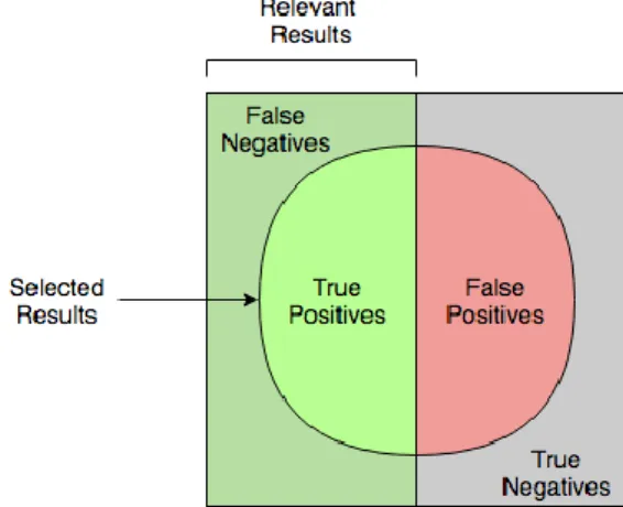
Precision (𝑝, or positive predictive value) is the percentage of correctly labeled positive results over all results, i.e., how many of the selected items are correct;
Recall (𝑟, also sometimes named coverage, sensitivity, true positive rate, or hit rate) refers to the percentage of correctly labelled positive results over all positive labelled cases, i.e., how many of the correct items were selected.
A system with high recall but low precision returns many results, most of which are incorrect when compared to the training labels. The contrary case is a system with high precision but low recall, which returns very few results, but most of its predicted labels are correct when compared to the training ones. An ideal system is the one that returns many results, all of which labelled correctly, achieving high precision and recall values.
Precision and recall can be described as a class match problem where the notion of true positive, true negative, false positive and false negative is required.
For a better understanding, table 2.1 shows a confusion matrix that relates each of these measures. The concepts presented are a result of the relation between the predicted class (the
one assigned in the process) and the golden class (the correct class/assignment).
Table 2.1 - Confusion matrix with evaluation measures
Predicted class
Golden class
Positive Negative
Positive True positive (TP) False positive (FP)
Negative False negative (FN) True negative (TN)
The stated concepts can be described as follows:
True Positive: If the identified class is correctly labelled, i.e., is present in the golden class.
True Negative: If the class is not present in the golden file, and the system, correctly, did not identify it.
False Positive: cases wrongly misclassified as positive (type I errors, incorrect cases), i.e., the identified class is not present in the golden file;
False Negative: cases missed or incorrectly rejected by the system (type II errors). The figure 2.2, presented below, may help the comprehension of these concepts.
Based on these concepts, one can see the measures previously described as follows:
𝑝 = 𝑇𝑃 𝑇𝑃 + 𝐹𝑃 (2.5) 𝑟 = 𝑇𝑃 𝑇𝑃 + 𝐹𝑁 (2.6)
Precision and recall are often combined into a single measure, the F-score (𝑓, also F1-score or
F-measure), which is the harmonic mean of precision and recall [35]. F-score reaches its best value at 1 (perfect precision and recall) and worst at 0, and can be represented as follows:
𝑓 =2 ∗ 𝑝 ∗ 𝑟 𝑝 + 𝑟 (2.7)
There are other metrics to consider. Accuracy (𝑎), for instance, is the fraction of correctly labelled (positive and negative) results over all results. Research in ML has put aside exhibiting accuracy results when performing an empirical validation of new algorithms. The reason for this is that accuracy assumes equal misclassification costs for false positive and false negative errors. This assumption is problematic, because for most real-world problems one type of classification error is much more expensive than another. For example, in fraud detection, the cost of missing a case of fraud is quite different from the cost of a false alarm [36].
Accuracy can be written following the same line of thoughts as precision and recall:
𝑎 = 𝑇𝑃 + 𝑇𝑁 𝑇𝑃 + 𝑇𝑁 + 𝐹𝑃 + 𝐹𝑁
(2.8)
One recommended metric when evaluating binary decision problems is Receiver Operator
Characteristic (ROC) curves, which show how the number of correctly classified positive
examples varies with the number of incorrectly classified negative examples [37]. An example of a ROC curve and how it should be interpreted is presented in the annex A, figure 1.
However, ROC curves can present an overly optimistic view of an algorithm’s performance if there is a significant skew in the class distribution. This can be addressed using Precision-Recall (PR)
curves. An example of a PR curve can be seen in subsection 2.6.3.5.
A precision-recall curve shows the trade-off between precision and recall for different thresholds. A high area under the curve denotes both high recall and high precision, where high precision represents a low false positive rate, and high recall a low false negative rate. High scores for both measures show that the classifier is retrieving accurate results (i.e., high precision), as well as a majority of all positive results (i.e., high recall).
The main difference between ROC space and PR space is the visual representation of the curves. In ROC space, the False Positive Rate (FPR) is plotted on the x-axis and the True Positive Rate (TPR) on the y-axis. In the PR space, the x-axis plots Recall, and the y-axis plots Precision. The goal in ROC space is to be in the upper left-hand corner; in PR space, the goal is to be in the upper-right-hand corner [38].
2.2.1.3.
Cross-Validation
provides a simple and effective method for both model selection and performance evaluation.
Ideally, there would be three different approaches to CV [40]:
1. In the simplest scenario, the user would collect one dataset and train the model via cross-validation to create the best model possible. Then, it would collect another utterly independent dataset and test it in the previously created model. However, this scenario is the most infrequent (given time, cost or most frequently dataset limitations).
2. If the user has a sufficiently large dataset, it would want to split the data and leave part of it to the side (i.e., completely untouched during the model training process). This is to simulate it as if it was a completely independent dataset, since a model that would repeat the labels of the samples that it has just seen would have a perfect score but would fail to predict anything useful on data not yet seen [26]. This event is called overfitting. To prevent it, the user would then build the model on the remaining training samples and test the model on the left-out samples.
3. Lastly, if the user is limited to a smaller dataset, it may not be able to ignore part of the data for model building simply. As such, the data is split into k folds, validation is performed on every fold (thus, the name k-fold cross-validation) and the validation metric would be aggregated across each iteration.
Since datasets are frequently small, k-fold cross-validation is the most used cross-validation method. Under it, the data is randomly divided to form k separated subsets of approximately equal size. In the ith fold of the cross-validation procedure, the ith subset is used to estimate the
generalised performance of a model trained on the remaining k−1 subsets. The average of the generalised performance observed over all k folds provides an estimate of the generalised performance of a model trained on the entire sample [41].
2.3. Controlled Vocabularies
In several fields of study, controlled vocabularies exist as a way to organise knowledge for subsequent retrieval of information. An example of knowledge classification is taxonomy13. The
end-user will most likely focus on one or more topic areas that can be summarised by a network of concepts and associations between them. These typically correspond to domain concepts which are found in thesauri and ontologies [42].
An ontology can be defined as “an explicit specification of a conceptualization” [43], thereby including representation, formal naming and/or definition of the categories, properties, and relations of the concepts, data, and entities that it covers. More formally, in information science, the word ontology is applied to a set of logical axioms that model a portion of reality [44].
The main strength in applying ontologies to data from different fields is the ease with which researchers can share information and process data using computers. As such, ontologies describe knowledge in a way that can be understood by humans and machines alike.
Because modelling ontologies are highly resource-consuming (given that are developed and described in logic-based languages like OWL), there is a preference to reuse existing models, like thesauri, as ontologies instead of developing ontologies from scratch. However, as Kless [45] stated, thesauri cannot be considered a less expressive type of ontology. Instead, thesauri and ontologies must be seen as two kinds of models with superficially similar structures. A qualitatively good ontology may not be a good thesaurus, the same way a qualitatively good thesaurus may not be a suitable ontology.
A thesaurus seeks to dictate semantic manifestations of metadata14 in the indexing of content
objects15 [46]. In other words, it assists the assignment of preferred terms to convey semantic
metadata associated with the content object, guiding both an indexer and a searcher in the selection of the same ideal term/combination of terms to represent a given subject.
The aim in using thesauri is to minimise semantic ambiguity by ensuring uniformity and consistency in the storage and retrieval of any manifestations of content objects.
2.3.1. Medical Subject Headings (MeSH)
The Medical Subject Headings (MeSH) thesaurus is a controlled vocabulary for the purpose of indexing, cataloguing and searching journal articles and books related to the life sciences [47].
It was first introduced by Frank Rogers, director of the NLM, in 1960 [48], with the NLM's own index catalogue and the subject headings of the Quarterly Cumulative Index Medicus (1940 edition) as precursors. Initially, it was intended to be a dynamic list, with procedures for recommending and examining the need for new headings [49]. Today it is used by MEDLINE/PubMed database and by NLM's catalogue of book holdings.
Many synonyms and closely related concepts are included as entry terms to help users find the most relevant MeSH descriptor for the concept they seek. In NLM's online databases, many search terms are automatically mapped to MeSH descriptors to ease the retrieval of relevant information.
2.3.1.1.
MeSH Structure
MeSH possesses three types of records [50]:
14 Data/information that provides information about other data. 15 Any item that is to be described.
i. Descriptors
Unit of indexing and retrieval. The MeSH descriptors are organised in 16 categories, from anatomic terms, organisms, diseases, and so on. Each category is further divided into subcategories. Within each subcategory, descriptors are arrayed hierarchically from most general to most specific in up to thirteen hierarchical levels. Because of the branching structure of the hierarchies, these are sometimes referred to as "trees" [51].
Each descriptor is followed by the number that indicates its tree location. For example, “C16.131” stands for “Congenital Abnormalities.”
ii. Qualifiers
Qualifiers offer a convenient means of grouping together citations which are concerned with a particular aspect of a subject. For example, “liver/drug effects” indicates that the article or book is not about the liver in general, but about the effect of drugs on the liver.
There are 81 topical Qualifiers (also known as Subheadings) used for indexing and cataloguing in conjunction with Descriptors.
iii. Supplementary Concept Records (SCRs)
Supplementary Chemical Records (SCRs), also called Supplementary Records, are used to index chemicals, drugs, and other concepts such as rare diseases for MEDLINE.
SCRs are not organised in a tree hierarchy; instead, each SCR is linked to one or more Descriptors by the Heading. They also include an Indexing Information (II) field that is used to refer to other descriptors from related topics. There are more than 230,000 SCR records, with over 505,000 SCR terms.
2.3.1.2.
Online Retrieval with MeSH
The MeSH Browser16, as an interactive Web application for searching and browsing MeSH data,
is the primary way of access to MeSH. However, as the MeSH browser only returns terms, these are to be used in databases such as PubMed.
The main method of using MeSH with PubMed is by providing the search engine with terms in MeSH records. To ensure a Pubmed search uses a MeSH term, the query should have the [mh] tag, for example, “Asthma [mh].” This query17 would retrieve every citation indexed with this
Descriptor since PubMed automatically searches on narrower Descriptors indented under the main Descriptor in the MeSH Tree Structures.
16 https://meshb.nlm.nih.gov/search
If the user has no idea what MeSH term or terms have been used in indexing relevant literature, a text word search may be performed first. For example, if a user is interested in "scalp diseases" - a term not in MeSH, they can search this term in PubMed (title and/or abstract). After seeing particularly relevant citations, the user can look at the citation record (MEDLINE format), and find the MH term “Scalp Dermatoses,” that will be the basis of a new query [52].
2.3.1.3.
Example
A quick search through the MeSH Browser allows the user to acquaint itself with the functioning of the database.
Taking “brain” as a search term, for instance. After the insertion of the term in the search box, a full report is displayed, as presented in figure 2 (in the annex B).
The first tab, “Details,” immediately shows the MeSH Heading and its tree number(s) in the first two lines, in this case, “brain” and “A08.186.211” respectively. The following lines present the related annotations, scope notes, entry terms, and other notes. The “Qualifiers” tab shows the related entry combination (for example, “chemistry:Brain Chemistry”) and allowable qualifiers (for example, “anatomy & histology (AH)”). The “MeSH Tree Structures” tab shows the location of the term, as well as the parent and child nodes (if available). For the referred term, the hierarchy tree is presented in figure 2.3.
The last tab, “Concepts,” shows the concepts related to the term in question, is this case the only concept is “Brain Preferred.”
2.4. Text Mining within Systematic Reviews
Several authors have widely studied the availability and utility of text-mining tools to support systematic reviews over time.
The application of TM techniques to support the citation screening stage of SRs is an emerging research field in computer science, with the first reported publication on the subject in 2005 by Aphinyanaphongs et al. [53]. Their research showed that using machine learning methods it was possible to automatically construct models for retrieving high-quality, content-specific articles in a given time period in internal medicine, that performed better than the 1994 PubMed clinical query filters.
A SR of 26 studies, performed by Pluye et al. [54], reiterates the statement that information-retrieval technology produces a positive impact on physicians regarding decision enhancement, learning, recall, reassurance, and confirmation of a given hypothesis.
In 2015, another SR of 44 papers by O’Mara-Eves et al. [9] pulled together the evidence base for the use of TM for CS. Whilst the authors found that it is difficult to establish any overall conclusions about the best approaches, they also suggested that the (semi)-automation of screening could result in a saving in workload of between 30% and 70%, though sometimes that saving is accompanied by a 95% recall (i.e., the loss of 5% of relevant studies).
Jonnalagadda et al. [8] later referred on their study that the data extraction step is one of the most time-absorbing of the SR process, and that TM techniques, more specifically NLP, may be an essential strategy to reduce the time implicated. Nonetheless, the authors point out that even though most NLP research has focused on reducing the workload for the CS step, biomedical NLP techniques have not been fully exploited to entirely or partially automate the SR process.
A challenge that was pointed by Paynter et al. [55] was that the creation of training datasets, given the comprehensive nature of the TM algorithm, given the comprehensive nature of the research performed, tends to include much more irrelevant than relevant citations, leading to “imbalanced datasets.” Olorisade et al. [56] also highlight that the lack of information about the datasets and machine learning algorithms limits the reproducibility of a high amount of published studies.
Even though TM tools are currently being used within several SR organizations for a variety of review processes (e.g., searching, screening abstracts), and the published evidence-base is growing fairly rapidly in extent and levels of evidence, Paynter et al. [57] acknowledge that text mining tools will be increasingly used to support the conduct of systematic reviews, rather than substituting current literature retrieval and information extraction tools. Some significant limitations presented by the authors are that many TM tools rely on corpora from PubMed/MEDLINE to train the learning algorithm, which does not represent the entire population of literature relevant for healthcare-related systematic reviews.
2.5. Related Tools
together with articles cited by the ACP Journal Club as a gold standard for the training of the algorithm. The authors chose this specific gold standard because of its focused quality review, that is highly regarded and uses stable explicit quality criteria.
In most of the studied categories, the data-induced models showed better or comparable precision, recall, and specificity than the pre-existing query filters. These results proved that, following this approach, it is possible to automatically build models for retrieving high-quality, content-specific articles in a given time period that performed better than the 1994 PubMed clinical query filters.
Rathbone et al. [58] evaluated the performance of Abstrackr, a semi-automated online tool for predictive title and abstract screening. The authors used four different SR to train a classifier, and then predict and classify the remaining unscreened citations as relevant or irrelevant. The results showed that the proportion of citations predicted as relevant by Abstrackr was affected by the complexity of the reviews and that the workload saving achieved varied depending on the complexity and size of the reviews. Still, the authors concluded that the tool had the potential to save time and reduce research waste.
Paynter et al. [55] conducted a research which goal was to provide an overview of the use of TM tools as an emerging methodology within some SR processes. This project culminated in a descriptive list of text-mining tools to support SR methods and their evaluation. The authors found two major TM approaches:
1. The first approach assessed word frequency in citations as presented by stand-alone applications, which generate frequency tables from the results set outlining the number of records by text word, controlled vocabulary heading, year, substances, among others. While this approach was used by Balan et al. [59], Kok et al. [60] and Hausner et al. [61] in their studies and applications, other authors used EndNote (a citation management application) to generate word frequency lists.
2. The second approach is automated term extraction. This approach also generates word frequency tables, but many were limited to single word occurrences. Tools such as AntConc18, Concordance19, and TerMine20 extract phrases and combination terms; other
applications such as MetaMap21 and Leximancer22 add a semantic layer to the process
by using tools provided through the NLM’s Unified Medical Language System.
18 http://www.laurenceanthony.net/software/antconc/ 19 http://www.concordancesoftware.co.uk 20 http://www.nactem.ac.uk/software/termine/ 21 https://metamap.nlm.nih.gov 22 https://info.leximancer.com
Even though the tools apply different algorithms, the overall approaches were similar. They start by creating a training set. In addition to that, another corpus representing the general literature (usually created by randomly sampling citations from PubMed) may be presented to the algorithm.
Only “overrepresented” words and phrases in the training set are considered for inclusion in the search strategy. Nonetheless, as noted by Petrova et al. [62] and O’Mara-Eves et al. [63], this approach has inherent problems: not only the reported frequencies for text words do not necessarily reflect the number of abstracts in which a word appears, but the term extraction algorithm also depends on the content of the documents supplied to it by the user/reviewer.
Most of the tools and studies examined by Paynter et al. [55] found benefit in automating term selection for SR, especially those comprising large unfocused topics. For example, in their study, Balan et al [59] concluded that “the benefits of TM are increased speed, quality, and reproducibility of text process, boosted by rapid updates of the results”; Petrova et al. [62] highlights the importance of word frequency analysis, since it “has shown promising results and huge potential in the development of search strategies for identifying publications on health-related values”.
2.6. Resources
This project is built on a wide range of Python packages, namely Biopython, NLTK, and Scikit-learn. The following subsections will describe each of them, relating them to their future role on this work.
2.6.1.
Biopython
The Biopython Project [64] is an international association of developers of freely available Python tools for computational molecular biology. Python is an object-oriented, high-level programming language with a simple and easy to learn syntax, which is why it is becoming increasingly popular for scientific computing. Thus, Biopython provides an online resource for modules, scripts, and web links for developers of Python-based software for bioinformatics use and research.
One of Biopython’s functionalities is the access to NCBI’s Entrez databases. Entrez23 is a data
retrieval system that provides users access to NCBI’s databases such as PubMed, GenBank, GEO, among others. Entrez can be accessed from a web browser to enter queries manually, or one can use Biopython’s Bio.Entrez module for programmatic access to Entrez, which allows searching PubMed from within a Python script.
After using Bio.Entrez to query PubMed, the result will be a Python list containing all of the PubMed IDs of articles related to the given query. If one wishes to get the corresponding Medline records and extract the information from them, it will be necessary to download the Medline
records in the Medline flat-file format and use the Bio.Medline module to parse them into Python utilisable data structures.
2.6.2.
NLTK
The Natural Language Toolkit, also known as NLTK [65], is an open source library, which includes extensive software, data, and documentation, that can be used to build natural language processing programs in Python. It provides basic classes for representing data relevant to natural language processing, standard interfaces for performing tasks such as syntactic parsing and text classification, and standard implementations for each task that can be combined to solve complex problems.
One of NLTK’s functionalities is the processing of raw text. For that, it requires a corpus. The
nltk.corpus Python package defines a collection of corpus reader classes, which can be used to
access the contents of a diverse set of corpora. An example of this is the
CategorizedPlaintextCorpusReader. It is used to access corpora that contain documents which
have been categorised for topic, label, etc. In addition to the standard corpus interface, these corpora provide access to the list of categories and the mapping between the documents and their categories.
After accessing the corpus, it is necessary to normalise it. NLTK provides tools to normalize text, from tokenization, the removing of punctuation, or converting text to lowercase, so that the distinction between “The” and “the,” for example, is ignored. Another resource NLTK provides is a set of stopwords, that is, high-frequency words like “the,” “to” and “also” that one sometimes wants to filter out of a document before further processing. Stopwords usually have little lexical content, and their presence in a text fails to distinguish it from other texts. Often it is still necessary to go further than this, so NLTK offers a way to Stemm and/or Lemmatize the raw text.
2.6.3.
Scikit-learn
Scikit-learn [26] is a free machine learning library for Python. It features various classification, regression and clustering algorithms including support vector machines, random forests, k-means and many others.
The Scikit-learn Application Programming Interface (API) is an object-oriented interface centered around the concept of an estimator — broadly any object that can learn from data, be it a classification, regression or clustering algorithm. Each estimator in Scikit-learn has a fit() and a
predict() method:
The fit() method sets the state of the estimator based on the training data. Usually, the data is comprised of a two-dimensional array X of shape “(nr. samples, nr. predictors)” that holds the feature matrix, and a one-dimensional array y that holds the labels; The predict() method generates predictions: predicted regression values in the case of


![Figure 3.5 - Search process and study selection flowchart (adapted from [71])](https://thumb-eu.123doks.com/thumbv2/123dok_br/19225412.964680/47.892.136.763.421.864/figure-search-process-study-selection-flowchart-adapted.webp)