Likelihood-based Inference for Multivariate Regression Models using Synthetic Data

(1)

Ricardo Pinto Moura

Licenciado em Matemática - Ramo Educacional

Likelihood-based Inference for Multivariate

Regression Models using Synthetic Data

Dissertação para obtenção do Grau de Doutor em

Estatística e Gestão do Risco

Co-orientadores: Carlos Agra Coelho, Associate Professor with Habilitation, Faculty of Sciences and Technology NOVA University of Lisbon

Bimal K. Sinha, Presidential Research Professor, University of Maryland Baltimore County

Júri

Presidente: Prof. Doutor José Paulo Barbosa Mota

Arguentes: Prof.aDoutora Maria Ivette Leal de Carvalho Gomes Prof. Doutor Pedro José Ramos Moreira de Campos Vogais: Prof. Doutor António Manuel Pacheco Pires

(2)

(3)

Likelihood-based Inference for Multivariate Regression Models

using Synthetic Data

(4)

(5)

(6)

(7)

Acknowledgements

Firstly, I would like to thank my adviser Prof. Dr. Carlos Agra Coelho for giving me the honor of being his advisee, for trusting me, for his great friendship and support and for giving the brightest advices every time. I would like to also thank my co-adviser Prof. Dr. Bimal Sinha for introducing me to the SDC world and to the multiple imputation technique that would be the foundation of this thesis, for trusting me the task of developing this work, for sharing with me his expertise and also for his friendship.

To my friends in the Centre of Mathematics and Aplications of the Nova Uni-versity of Lisbon, for making me feel at home in the center and for their support. To UMBC staffand students for welcoming me to their family and to make me

a member of that family.

To Fulbright, by choosing me for the Research Grant which allowed me to build the core work near the Prof. Dr. Bimal Sinha at UMBC and for allowing me to experience the culture of the U.S.A..

To Dr. Martin Klein, for letting me be in his Statistical Computing classes and for his support.

To my parents, for their sacrifice in all the rough times showing that there’s no gain without work.

(8)

(9)

Abstract

Likelihood-based exact inference procedures are derived for the multivari-ate regression model, for singly and multiply imputed synthetic data genermultivari-ated via Posterior Predictive Sampling (PPS), via a newly proposed sampling method, which will be called Fixed-Posterior Predictive Sampling (FPPS), and via Plug-in sampling. By contemplating the single imputation case, the new developed pro-cedures fill the gap in the existing literature where inferential methods are only available for multiple imputation and, by being based in exact distributions, it may even be applied to cases where the sample size is small. Simulation studies compare the results obtained from all the proposed exact inferential procedures and also compare these with the results obtained from the adaptation of Reiter’s combination rule to multiply imputed synthetic datasets. An application using U.S. 2000 Current Population Survey data is discussed and measures of privacy are presented and compared among all methods.

(10)

(11)

Resumo

Procedimentos inferenciais baseados em funções de verosimilhança são dedu-zidos para o Modelo de Regressão Linear Multivariado, para dados sintéticos de imputação única e de imputação múltipla gerados viaPosterior Predictive Sampling (PPS), via um novo método, que se denominará porFixed-Posterior Predictive Sam-pling(FPPS), e viaPlug-in Sampling. Ao contemplar o caso de imputação única, os novos procedimentos desenvolvidos preenchem um vazio na literatura existente onde métodos inferenciais estão disponíveis exclusivamente para casos de impu-tação múltipla e, como se baseiam em distribuições exatas, podem ainda assim ser aplicados a casos onde a dimensão da amostra é pequena. O estudo de simulações permite a comparação de todos os resultados provenientes dos procedimentos exatos propostos como também a comparação destes com os resultados obtidos aquando da aplicação da regra combinatória de Reiter a dados sintéticos de múl-tipla imputação. É discutida uma aplicação usando dados daU.S. 2000 Current Population Surveye medidas de privacidade são apresentadas e comparadas entre todos os métodos.

(12)

(13)

List of Figures

2.1 Smothed Empiricaldistributionsandcut-offpoints (_γ=0_.05) of_T•

1,T2•,

T₃•andT₄•forρ=0.2,0.4,0.6,0.8. . . 16

3.1 Smoothed empiricaldistributionsandcut-offpoints (_γ=0_.05) of_T∗

1,T2∗,

T₃∗andT₄∗ forρ=0.2,0.4,0.6,0.8. . . 37

5.1 Histograms (with same vertical scale) of the empirical distributions of T_M† for M = 2 and 5 (for m = 3, p = 24, n = 141, α = 8 and 104

simulation sizes). . . 68 5.2 Histograms (with same vertical scale for eachM) of the empirical

dis-tributions of bothT_M• andT_comb• for M= 1,2 and 5 (form= 3,p = 24, n= 141,α= 8 and 104simulation sizes). . . 68

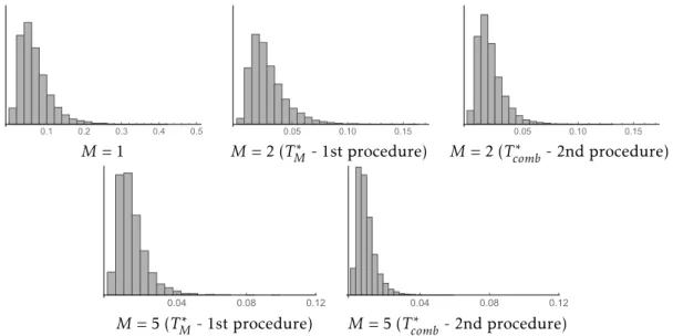
5.3 Histograms (with same vertical scale for eachM) of the empirical

dis-tributions of bothT_M∗ andT_comb∗ for M= 1,2 and 5 (form= 3,p = 24, n= 141 and 104simulation sizes). . . 68

5.4 Box-plots of p-values obtained, when testing the joint significance of I(R=2), I(R=4) and I(S=2), from 100 draws of synthetic datasets using PPS, FPPS and Plug-in Sampling method as also when using Reiter’s adapted combination rule forM= 1,M = 2 andM= 5 . . . 70

(16)

(17)

List of Tables

2.1 Cut-offpoints of the 95% confidence set for the regression coefficients matrix B. . . 19

3.1 Cut-off_{points of the 95% confidence set for the regression coe}ffi_{cients matrix} B. . . 41

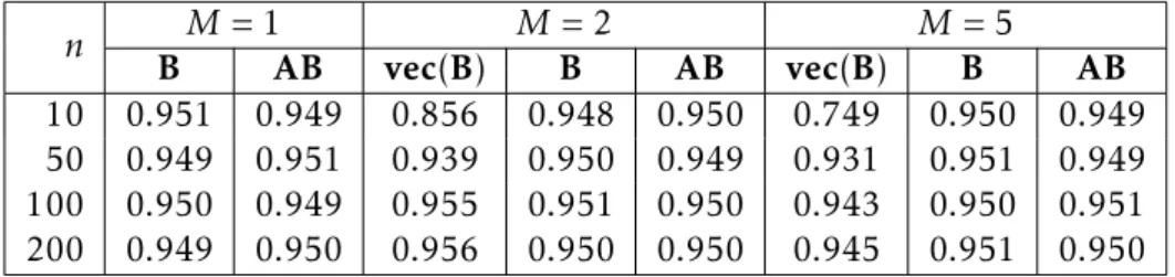
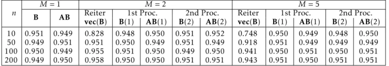
4.1 Estimated coverage probability forvec(B),BandABunder PPS.. . . 59 4.2 Estimated coverage probability forBandABunder FPPS. . . 60 4.3 Estimated coverage probability forvec(B),BandABunder Plug-in Sampling. 60 4.4 Average values of theradiuswhen using FPPS and Plug-in Sampling with the

corresponding expected values and the values ofΥ†

M,minandΥM,max† defined

in (4.9) and (4.8) when using PPS, for the confidence set forB. . . 61 4.5 Average values of theradiuswhen using FPPS and Plug-in Sampling with the

corresponding expected values and the values ofΥ†

M,minandΥM,max† defined

in (4.9) and (4.8) when using PPS, for the confidence set forC. . . 61

5.1 Summary of CPS data variables. . . 64 5.2 Estimates of the regressor coefficients from the synthetic data and from the

original data. . . 66 5.3 Approximated values of the cut-offpoints computed from the empirical

dis-tributions ofT_M†,T_M•,T_comb• ,T_M∗ andT_comb∗ respectively defined in subsections 2.2.2, 2.3.1, 2.3.2, 3.2.2 and 3.2.3, forγ= 0.05. . . 69 5.4 Power for the test to the hypothesis (5.3), withB(1) andB(2) denoting the

first and second procedures developed in Chapters 2 and 3, for the FPPS, PPS (only one procedure is available) and Plug-in methods, withvec(B) denoting Reiter’s adapted procedures. . . 73 5.5 Power for the test to the hypothesis (5.4), withC(1) andC(2) denoting the

(18)

L i s t o f T a b l e s

5.7 Values ofΓ₃_,₀_.₁and a summary of the distribution of_D₃. . . 76

(19)

Listings

A.1 Example of source code for the empirical distribution ofT_M† defined

in (2.27) used in the CPS application. . . 88 A.2 Example of source code for the empirical distribution of T_M• and

T_comb• respectively defined in (2.32) and (2.40), used in the CPS

application.. . . 89 A.3 Example of source code for the empirical distribution of T_M∗ and

T_comb∗ respectively defined in (3.11) and (3.15), used in the CPS

(20)

(21)

C

h

a

p

t

e

r

1

General Introduction

«In intelligence work,[. . . ] there are limits to the amount of information one can share. Confidentiality is essential[. . . ].»

Gijs de Vries

1.1 Introduction

When releasing microdata to the public, methods of statistical disclosure control (SDC) are used to protect confidential data, that is “data which allow statistical units to be identified, either directly or indirectly, thereby disclosing individual information” [29], without compromising an adequate and accurate statistical analysis of the data. Several SDC methods have been recently developed in order to protect the data, without changing its fundamental structure.

(22)

C H A P T E R 1 . G E N E R A L I N T R O D U C T I O N

Recoding, suppression, top and bottom coding are classified as non-perturbative [5,9,12].

With these methods one faces the problem that some released data guaran-tees respondents confidentiality but researchers may not accept it due to dubious quality or the problem that in order to have high quality data, respondents sensi-tive information could be put in high risk of disclosure. With the synthetic data approach, which has gained considerable popularity and importance in recent times, these problems can be overcome [21,37].

Little [24] and Rubin [36], in 1993, first supported the use of synthetic data for SDC, using the framework of multiple imputation [35]. Rubin claimed that synthetic data so created do not correspond to any actual sampling unit, thus preserving the confidentiality of the respondents. Rubin also proposed that one could use fitted models to generate random and independent samples of the orig-inal survey data and release these synthetic versions of microdata publicly, called fully synthetic datasets. The quality of this approach is dependent on the model to impute the values, therefore, all the relationship between variables must be included and the joint distribution of these has to be specified, in order to not give biased results when using the synthetic data [5,6]. Later that year, Little [24] proposed to only replace, with imputed values, the observed values that could contain sensitive information, leaving the rest unchanged, a proposed solution to overcome the problems inherent to the creation of fully synthetic datasets. This approach is called generation of partially synthetic datasets. This will be the context of the present work. In 1997, Kennickell [14] was the first to use multiply-imputed partially synthetic data to protect the confidentiality of respondents in the Survey of Consumer Finances. Only in 2003, inferential methods for fully synthetic data were developed by Raghunathan et al [27], while, at the same time, Reiter [30] presented the first methods for drawing inference for partially syn-thetic data.

In comparison with the standard SDC methods, multiple imputation tech-niques presents many advantages dealing with many real data problems that other methods cannot. It preserves the joint distribution of the original data of-fering a better quality analysis; is applicable to both categorical and continuous variables; released fully synthetic datasets gives a very small disclosure risk; with partially synthetic datasets generation one may only synthesize the records at risk, maintaining intact the records that have no need to be protected; it allows the possibility to impute missing values before generating synthetic datasets having

(23)

1 . 1 . I N T R O D U C T I O N

no need to give up on some records; preserves linear constraints; allows the ana-lyst to decide if valid results will be given from the synthetic data based on the meta-data information. Some drawbacks exist as well. Since it is a perturbation method there is a question on the utility limit of the data and only the statistical properties gathered by the model are preserved [2,5].

The most common methods to synthesize data are the Posterior Predictive Sampling and Plug-in Sampling. Although most inferential methods for synthetic data are based on multiple imputation, Klein and Sinha [17,18,19,20] in a series of recent papers developed exact parametric inferential methods based on singly imputed synthetic data for several probability models, including the multiple linear regression model where the sole response variable is considered sensitive, thus requiring protection, while the covariates are treated as non-sensitive, having no need of confidentiality protection.

The main goal of this thesis is to extend this scenario to the multivariate linear regression model where there are multiple sensitive responses variables follow-ing a multivariate normal distribution with expected values modeled as linear combinations of multiple non-sensitive covariates. Based on the fitted multi-variate linear regression model, the sensitive responses are synthesized based on the Posterior Predictive Sampling method, Plug-in Sampling method and on a new proposed sampling method that will be called Fixed-Posterior Predictive Sampling, and exact data analysis procedures are developed for both single and multiple imputation, for all methods. Reiter [30,31] combining rules for scalar and vector parameters are the most commonly used methodologies in the analysis of released multiply imputed synthetic datasets [1,4,8,13,20], due to its easy applicability to various statistical models, as such, in this thesis, one will compare the new developed inferential procedures with the adaptations of Reiter’s [31] methodology to Posterior Predictive Sampling and Plug-in Sampling multiply imputed synthetic data, under the Multivariate Linear Regression model. The contents of this thesis are as follows:

• In Chapter2, based on singly imputed synthetic data generated via Posterior Predictive Sampling, an exact inferential procedure is developed for the matrix regression coefficients_B. Based on multiply imputed synthetic data

(24)

is contrasted with Reiter’s asymptotic methodology adaptation for multiple imputation synthetic data [31]. It is also shown that pivot statistics based in the classical test statistics forBunder Multivariate Linear Regression model are not pivotal for imputed synthetic data generated via Posterior-Predictive Sampling.

• In Chapter3, an exact inferential procedure for the matrix of regression co-efficients_Bis developed based on singly imputed synthetic data generated

via Plug-in Sampling. Based on multiply imputed synthetic data, two exact inference procedures are developed and compared with Reiter’s asymptotic methodology adapted to multiply imputed synthetic data. It is also shown that pivot statistics based on the classical test statistics forBunder the Mul-tivariate Linear Regression model are also not pivotal for imputed synthetic data generated via Plug-in Sampling.

• In Chapter4, it is proposed a measure, theradius, that measures the distance between the center and the edge of the confidence sets for the regression coefficients matrix_B. Simulation results corroborate the accuracy of the

the-oretically derived results for the singly imputed and multiply imputed syn-thetic datasets. These are compared with the results from Reiter’s adapted procedures. Values for the confidence sets radius for all new procedures developed in Chapters2and3are also compared.

• Chapter5presents data analyses under the proposed methods for singly and multiply imputed synthetic data in the context of public use data from the 2000 U.S. Current Population Survey. The results are compared with those obtained from the original data. Using the same public use data, the levels of Privacy Protection for single and multiple imputation released synthetic data for all sampling methods used in Chapters2and3are compared.

• A general discussion of the main results and conclusions is presented in Chapter6.

1.2 Generating Synthetic Data

In order to generate synthetic data for the purpose of public release, the tech-niques used throughout this thesis will be the Posterior Predictive Sampling (PPS), a new adapted method that we will call Fixed-Posterior Predictive Sam-pling (FPPS) and the Plug-in SamSam-pling.

(25)

1 . 3 . T H E M U LT I VA R I AT E L I N E A R R E G R E S S I O N M O D E L

Brief descriptions of the three techniques are presented in the following sub-sections where we consider that Y = (y1, . . . ,yn) are the original data which are

jointly distributed according to the probability density function (pdf)fθ(Y), where

θ is the unknown (scalar, vector or matrix) parameter.

1.2.1 Posterior Predictive Sampling (PPS)

A priorπ(θ) forθ is assumed and then the posterior distribution ofθ is obtained as π(θ_|_Y)_∝_π(θ)_f_θ, and used to draw _M independent estimates θ•₁_{, . . . ,}θ•

M ofθ.

Following, M replacements ofYare generated, namely, W_j =w_j1, . . . ,wjn

, j =

1, . . . , M,drawn all independently from the correspondingj-th pdffθ•

j, wherefθ•j

is the pdf of Y where the originalθ is replaced by θ•

j, for j = 1, . . . , M. These

synthetic datasets W_j (j = 1, . . . , M) will be the datasets available to the general

public.

1.2.2 Fixed-Posterior Predictive Sampling (FPPS)

A priorπ(θ) forθ is assumed and then the posterior distribution ofθ is obtained as π(θ_|_Y) _∝ _π(θ)_fθ, and used to draw just one estimate of θ, θ•

f. Then, one

generatesMreplacements ofY, namely,Wj=

wj1, . . . ,wjn

, j = 1, . . . , Mdrawn all

independently from the same fθ•

f, where fθ

•

f is the pdf of the original Y where

θ•

f replaces the originalθ. These synthetic datasetsWj (j = 1, . . . , M) will be the

datasets available to the general public. One may observe that, forM= 1, both the

Posterior Predictive Sampling and the new Fixed-Posterior Predictive Sampling methods concur.

1.2.3 Plug-in Sampling

We start by taking the value of a point estimator ˆθ(_Y) ofθ, and plug it into the joint pdf ofY. The resulting pdf, with the unknownθ replaced by the observed value of the point estimator ˆθ(_Y), is denoted by _f_θ_ˆ. The multiply imputed syn-thetic datasets, denoted by W_j(j = 1, . . . , M), are then generated independently

by drawingW_j =w_j1, . . . ,wjn

from the joint pdffθˆ and these synthetic datasets

W_j(j= 1, . . . , M) will be the datasets available to the general public.

1.3 The Multivariate Linear Regression Model

(26)

this model in the context of partially-synthetic data analysis and define the test statistics that will be used for the original data.

Considermsensitivevariablesy_j, j = 1, . . . , m, that should be replaced by their

synthetic version because they present a risk to respondents confidentiality, origi-nating the vector y = (y1, . . . , ym)′, and a set of p non-sensitive variables x=x1, . . . , xp

′

, that do not need to be protected.

In terms of the MLR model,y= (y1, . . . , ym)′ will be considered the vector of

response variables andx=x1, . . . , xp ′

the set of predictor variables or covariates. We will consider thaty|_x∼Nm(B′x,Σ), withBand Σunknown, and the

orig-inal data will consist of Y=n(y1i, . . . , ymi, x1i, . . . , xpi), i= 1, . . . , n o

, observing that predictor variables are considered fixed. Let us write Y = (y1, . . . ,yn) with yi =

(y1i, . . . , ymi)′ and X = (x1, . . . ,xn) with xi = (x1i, . . . , xpi)′, assuming that rank(X : p×n) =p < nandn≥m+p. Therefore we have the following regression model

Y_m×n=B′m×pXp×n+Em×n (1.1)

whereE_m×nwill be distributed asNmn(0,In⊗Σ).

The maximum likelihood estimator (MLE) and uniformly minimum-variance unbiased estimator (UMVUE) ofB, distributed asN_pmB,Σ_⊗(_XX′)−1

ˆB= (XX′)−1_XY′_, _(1.2)

independent of

ˆ

Σ= 1

n

Y− ˆB′X Y− ˆB′X′ (1.3)

which is the MLE ofΣ, with_nΣˆ _∼_W

m(Σ, n−p) [3, Chapter 8]. ThereforeS= n

ˆ

Σ n−p

will be an unbiased estimator (UE) ofΣ.

Several tests forB based on the original data can be found in the literature [3, Chapter 8], but, as it will be shown in the next Chapter, the adaptations of this classical tests to the synthetic data cannot be used, therefore, for purposes of comparison, it is developed a new test procedure for Band also for C=AB,

whereAis ak×pmatrix withrank(A) =k≤pandk ≥m. Inference based on the

original data will be drawn and will be used to compare with inference drawn from the synthetic data. This test procedure will be based on

T_O =

_Bˆ ₋_B′₍_XX′₎_Bˆ ₋_B

|(n−p)S| ∼

m Y

i=1

p−i+ 1

n−p−i+ 1Fi (1.4)

and

T_O,C=

ABˆ −C′A(XX′₎−1_A′−1_A_Bˆ ₋_C

|(n−p)S| ∼

m Y

i=1

k−i+ 1

n−p−i+ 1Fk,i (1.5)

(27)

1 . 4 . A N I M P O R TA N T L E M M A

whereFi (i = 1, . . . , m) andFk,i (i = 1, . . . , m) are two sets of independent random

variables following respectivelyF_p−i+1,n−p−i+1andFk−i+1,n−p−i+1distributions. The derivation of the distributions ofT_O andT_O,Ccan be seen in AppendixA.

1.4 An important Lemma

Concluding this Chapter, it will be important for the derivation of all the results developed in Chapters2and3to make an observation regarding the existence of sufficient statistics.

Suppose the original data areY∼fθˆ₍_Y₎, and the synthetic dataV = (V1, . . . ,V_M) are generated such that V1|Y, . . . ,VM|Y are independent and identically

distributed (i.i.d.) fromfθˆ(_Y). Suppose thatT(Y) is a sufficient statistic forθbased on the original data. Then the pdf of the synthetic dataV = (_V₁_{, . . . ,}_V_M) is

Z _YM

i=1

fθˆ(_Y)(V_i)

fθ(Y)dY=

Z _YM

i=1

gθˆ(_Y)(T(V_i))h(V_i)

fθ(Y)dY

=

M Y

i=1

h(V_i) Z

M Y

i=1

gθˆ₍_Y₎(T(V_i))

fθ(Y)dY,

wheregθˆ₍_Y₎(T(V_i)) andh(V_i) are non-negative functions, withg depending onV_i only through the statisticT(V_i) andhonly depending onV_i, which implies the following result.

Lemma 1.4.1. Suppose that when the original dataY are observed, T(Y) is a suffi -cient statistic for θ_{. Then when the synthetic data} V = (_V₁_{, . . . ,V}_M) _{are observed,}

(T(V1), . . . ,T(VM)) is jointly sufficient forθ. Furthermore, if M = 1, the sufficient

(28)

(29)

C

h

a

p

t

e

r

2

Inference for Multivariate

Regression Model based on

synthetic data generated via PPS

and FPPS

The main objective of this chapter is to present the likelihood-based approach developed for the analysis of partially-synthetic data generated via Posterior Pre-dictive Sampling (PPS) and via a new proposed sampling method called Fixed-Posterior Predictive Sampling (FPPS) which is originated from an adaptation of the PPS method.

When one uses the PPS method to generate the multiply imputed synthetic data one has to deal with the problem of obtaining the distribution of a sum of Wishart distributions with different parameters. The use of the FPPS method is

suppose to overcome this problem.

Most of the content of Sections 2.1 and 2.3 is taken from [25].

2.1 Posterior Predictive Sampling (PPS)

(30)

C H A P T E R 2 . I N F E R E N C E FO R M U LT I VA R I AT E R E G R E S S I O N M O D E L BA S E D O N S Y N T H E T I C DATA G E N E R AT E D V I A P P S A N D F P P S

developed asymptotic based inferential procedures to analyze multiply imputed synthetic data using the PPS method to generate these synthetic data. All these inferential procedures are only suitable for the analysis of multiply imputed syn-thetic datasets leaving a gap in the state of art by leaving out the single imputation case. Since, in some cases [11,15,16] it is mandatory to only release one single synthetic data due to the high risk of disclosure, it is important to make available an inference procedure for this case.

2.1.1 Single Imputation: Posterior Predictive Sampling Method

The PPS method was generally described in subsection1.2.1. In this subsection, we will start by describing specifically the PPS method under the MLR model case.

Let us consider the MLR model (1.1) withY,X,B,Σ, ˆBand_Sdefined in that

same context. Consider the joint prior distribution

π(B,Σ)_{∝ |}Σ_|−α/2

and from it let us develop the posterior distributions for the unknown parameters

Σ and _Bin model (1.1). Let us observe that_Y_|_B

,Σ ∼N_mn(B′X,I_n⊗Σ). Hence the

likelihood function forYwill be

l(B,Σ_|

Y)∝ |Σ|−n/2e− 1

2tr{Σ−1(Y−B′X)(Y−B′X)′}_,

and the joint posterior distribution for (B,Σ) can be obtained from the product of

the previous prior and likelihood functions

π(B,Σ_|_Y)_{∝ |}Σ_|−n+2α_e−12tr{Σ−1(Y−B′X)(Y−B′X)′}_.

Regarding the exponent part of this joint posterior distribution, we may de-compose it as

trnΣ−1(_Y₋_B′_X)(_Y₋_B′_X)′o=_trnΣ−1(_Y₋ ˆB′_X+ ˆB′_X₋_B′_X)(_Y₋ ˆB′_X+ ˆB′_X₋_B′_X)′o

=trnΣ−1h(_Y₋ ˆB′_X)(_Y₋ ˆB′_X)′io

+trnΣ−1h(_Y₋ ˆB′_X)(ˆB′_X₋_B′_X)′+ (ˆB′_X₋_B′_X)(_Y₋ ˆB′_X)′+ (ˆB′_X₋_B′_X)(ˆB′_X₋_B′_X)′io

=trnΣ−1h(_Y₋ ˆB′_X)(_Y₋ ˆB′_X)′i+ (_B₋ ˆB)′(_XX′)(_B₋ ˆB)o

+ 2trnΣ−1h(_Y₋ ˆB′_X)(ˆB′_X₋_B′_X)′io_.

(31)

2 . 1 . P O S T E R I O R P R E D I C T I V E SA M P L I N G ( P P S )

Note that 2trnΣ−1h(_Y₋ ˆB′_X)(ˆB′_X₋_B′_X)′io is null, since ˆB′ = h(_XX′)−1_XY′i′ =

YX′₍_XX′₎−1_{and so}

Y− ˆB′X ˆB′X−B′X′=YX′ˆB−YX′B+ ˆBXX′_ˆB₊ _ˆBXX′_B

=YX′ˆB−YX′B+YX′(XX′)−1_XX′_ˆB₊_YX′₍_XX′₎−1_XX′_B

=YX′ˆB−YX′B−YX′ˆB+YX′B= 0,

therefore obtaining the posterior distribution proportional to

|Σ_|−n+α2−p_e−n−2ptr{Σ−1S} |Σ_|−p2_e−12tr{Σ−1(B−ˆB)′(XX′)(B−ˆB)}_,

by recalling the definition ofSasS=_n1₋_p(Y− ˆB′X)(Y− ˆB′X)′_.

Using Corollary 2.4.6.2. in [22], the posterior distribution forΣis given by

Σ_|_S_∼_W−1

m

(n−p)S, n+α−p, (2.1)

whereW_m−1(Ψ_{, ν}) denotes the Inverse Wishart distribution withΨ:_m_×_ma

posi-tive definite matrix andν degrees of freedom, and the posterior distribution for Bis given by

B|_ˆB_,Σ∼N_pm

ˆB,Σ_⊗(_XX′)−1 (2.2)

assumingn+α > p+m+ 1.

Now, it is possible to generate the synthetic dataset under the MLR model. Start by drawing Σ˜ from (2.1) and _B˜ from (2.2), upon replacing Σ byΣ˜ in this

latter expression, and then generate one single synthetic dataset, denoted asW= (w1, . . . ,wn) wherewi= (w1i, . . . , wmi)′, will be independently distributed as

w_i|_B˜_,Σ˜ ∼Nm _˜

B′x_i,Σ˜_{, i}= 1_{, . . . , n.} (2.3)

Let us define

B•= (XX′)−1XW′ (2.4)

and

S•= 1

n−p

W−B•′X W−B•′X′, (2.5)

that will be the estimators ofBandΣ, respectively. By Lemma1.4.1these

estima-tors are jointly sufficient. Note that conditionally on_B,˜ Σ˜,_B• is independent of

S•_{, as in the original data} _ˆB_and_S_{were also independent.}

(32)

Theorem 2.1.1. The joint pdf ofB•,S•andΣ˜−1_{, for}_B• _and_S• _{respectively defined in}

(2.4) and (2.5), is proportional to

e−

1 2tr

(2Σ˜+Σ)−1(_B•−B)′_XX′₍_B•₋_B₎₊₍_n₋_p₎Σ˜−1_S•

× |S

•_|(n−p)−₂m−1

|Σ˜_|(n−p)+2n+α−m−1

|Σ_|−n2

1 2Σ˜

−1₊_Σ−1

−p/2

Σ˜−1+Σ−1−

2n+α−2p−m−1

2 _. _(2.6)

Proof. GivenΣ˜ and_B˜ respectively from (2.1) and (2.2), we have that

W′|_B˜_,Σ˜ ∼Nnm

X′B,˜ Σ˜ _⊗_I

n

=⇒ B•|_B˜_,Σ˜ = (XX′)−1XW′|_B˜_,Σ˜ ∼Npm

˜

B,Σ˜ _⊗(_XX′)−1

and

(n−p)S•|Σ˜ ∼Wm

˜

Σ_{, n}₋_p_.

SinceB• _and_S•_{are independent, the conditional joint pdf of (}_B•_,_S•_{), given ˜}_B

and ˜Σ, will be proportional to

e−12tr{Σ˜−1[(B•−B˜)′XX′(B•−B˜)+(n−p)S•]} |S

•_|(n−p)−₂m−1

|Σ˜_|(n−p2)+p

, (2.7)

while, due to the independence of_B˜ _andΣ˜−1 drawn respectively from (2.2) and

(2.1), the joint pdf of (_B,˜ Σ˜−1), given_S, is proportional to

|Σ˜_|−p/2_e−21tr{Σ˜−1[(B˜−ˆB)′XX′(B˜−ˆB)+(n−p)S]} |S|

n+α−p−m−1 2

|Σ˜_|n+α2−p−m−1

. (2.8)

Given the independence of ˆBandS, defined in (1.2) and (1.3), the joint pdf of

(ˆB,S) is proportional to

e−12tr{Σ−1[(ˆB−B)′XX′(ˆB−B)+(n−p)S]} |S|

n−p−m−1 2

|Σ_|n2 . (2.9)

Thus, by multiplying the three pdf’s (2.7), (2.8) and (2.9), the joint pdf of

B•_,_S•_,_B,_˜ _Σ_˜−1_, _ˆB,_S_{is obtained.}

Since

trB•−B˜′XX′B•−B˜=trB˜−B•′XX′B˜−B•,

and since from (A.1) in Result A.2.1,

_˜

B−B•′XX′B˜ −B•+_B˜ ₋ _ˆB′_XX′_B_˜₋ _ˆB₌

= 2_B˜ −1

2

B•+ ˆB′XX′

˜ B−1

2

B•+ ˆB+1 2

B•−ˆB′XX′B•−ˆB,

(33)

the joint pdf of (B•,S•,Σ˜−1_, ˆB,_S) is obtained by integrating out_B˜, being

propor-tional to

e−12tr{Σ˜−1[12(B•−ˆB)′XX′(B•−ˆB)+(n−p)(S•+S)]+Σ−1[(ˆB−B)′XX′(ˆB−B)+(n−p)S]}

× |S

•_|(n−p)−₂m−1

|Σ˜_|(n−p)+2n−α−m−1

|S|n+α2−p−m−1

|Σ_|n2 . (2.10)

Taking into account that

tr ₁

2Σ˜

−1_B•₋ _ˆB′_XX′_B•₋ _ˆB₊_Σ−1_ˆB₋_B′_XX′_ˆB₋_B₌

=tr

XX′1

2

B•− ˆBΣ˜−1_B•₋ ˆB′+ˆB₋_BΣ−1ˆB₋_B′

and from (A.2) in Result A.2.2,

1 2

B•− ˆBΣ˜−1_B•₋ ˆB′+ˆB₋_BΣ−1ˆB₋_B′=

=

" ˆB−

₁

2B

•_Σ_˜−1₊_B_Σ−1 1

2Σ˜

−1₊_Σ−1−1# 1

2Σ˜

−1₊_Σ−1

" ˆB−

₁

2B•Σ˜−1+BΣ−1 1

2Σ˜−1+Σ−1

−1#′

+ (B•−B)2Σ˜ +Σ−1(_B•₋_B)′_,

integrating out ˆB, the joint pdf ofB•,S•,Σ˜−1_,_Swill be proportional to

e−12tr{(2Σ˜+Σ)−1(B•−B)′XX′(B•−B)+(n−p)Σ˜−1(S•+S)+(n−p)Σ−1S}

× |S

•_|(n−p)−₂m−1

|Σ˜_|(n−p)+2n−α−m−1

|S|n+α2−p−m−1

|Σ_|n2

1 2Σ˜

−1₊_Σ−1

−p/2

.

Consequently, integrating outSone ends up with the joint pdf ofB•_,_S•_,_Σ_˜−1

proportional to (2.6), concluding the proof.

In expression (2.6), one may see that S• _and _B•_{, conditionally on} _Σ_˜−1_{, are} separable, with

B•|Σ˜ ∼N_pm

B,(2Σ˜+Σ)_⊗(_XX′)−1 (2.11)

and

S•|Σ˜ ∼Wm

1

n−pΣ˜, n−p !

, (2.12)

(34)

Immediately from pdf (2.6), we may conclude that the MLE ofBbased on the synthetic data will beB•_{, with}

E(B•) = (XX′)−1XE(W′) = (XX′)−1_XX′_E_B_˜₌_E_ˆB₌_B,

therefore makingB• _{an UE. Its variance may be derived from} V ar(B•) =V arhE(B•|B,˜ Σ˜)i+_Eh_{V ar}(_B•_|_B,˜ Σ˜)i_,

where, forn+α > p+ 2m+ 2,

V arhE(B•|B,˜ Σ˜)i=_{V ar}h_B˜i=_{V ar}h_E(_B˜_|ˆB,Σ˜)i+_Eh_{V ar}(_B˜_|ˆB,Σ˜)i

=V ar(ˆB) +EhΣ˜ _⊗(_XX′)−1i=Σ_⊗(_XX′)−1+ n−p

n+α−p−2m−2Σ⊗(XX

′₎−1

and

EhV ar(B•|B,˜ Σ˜)i=_EhΣ˜ _⊗(_XX′)−1i= n−p

n+α−p−2m−2Σ⊗(XX

′₎−1_,

thus yielding

V ar(B•) =2(n−p−m−1) +n−p+α

n+α−p−2m−2 Σ⊗(XX

′₎−1_,

under the condition thatn+α > p+ 2m+ 2.

We may also observe thatS•is an UE ofΣ, if_α= 2_m₋2, since

E(S•) =E(Σ˜) =_E n−p

n+α−p−2m−2S

!

= n−p

n+α−p−2m−2Σ.

This way, having access only to one released synthetic dataset it is simple to compute estimates for the unknown parameters from the usual estimators.

At this point one could suggest, in order to perform tests forB, the following adaptations of the classical test criteria for the multivariate regression model (see [3, Secs 8.3 and 8.6] for the classical criteria):

(a) T₁•=|S•|S•+ (B•−B)′₍_XX′₎₍_B•₋_B₎−1 _{(Wilks’ Lambda Criterion);}

(b) T₂•=trn(B•−B)′₍_XX′₎₍_B•₋_B₎₍_S•₎−1o_{(Pillai’s Trace Criterion);}

(c) T₃• = trn(B•−B)′₍_XX′₎₍_B•₋_B_)[(_B•₋_B₎′₍_XX′₎₍_B•₋_B_{) +}_S•_]−1o _(Hotelling -Lawley Trace Criterion);

(35)

(d) T₄• = λ1 where λ1 denotes the largest eigenvalue of (B•−B)′(XX′)(B•−

B)(S•₎−1_{(Roy’s Largest Root Criterion).}

However, these statistics are non-pivotal, that is, their distributions will be func-tion of Σ. When using the term ‘statistic’ we are assuming _B known. In fact,

Lehmann in [23, Sec. 8.4] said that the distributions of these classical test statistics will depend only on the nonzero roots of the equation|E−λΣ_|= 0 thus implying

that their distribution will depend onΣ. Therefore, it is expected that the adapted

statistics in (a)-(d) for the analysis of synthetic data will also have distributions that will be function ofΣ. Considering this fact, let us begin by rewriting all four

classical statisticsT₁•,T₂•,T₃•andT₄•, in order to make them assume the same type

of form and then prove why all of them are non-pivotal. Let us consider

H=2Σ˜ +Σ−

1 2₍

B•−B)′(XX′)(B•−B)2Σ˜+Σ−

1

2 _(2.13)

and

G= (n−p)Σ˜−21_S•Σ˜−12_. (2.14) By Theorem 2.4.1 in [22], forp≥m,

(B•−B)′₍_XX′₎₍_B•₋_B₎_|

˜

Σ−1∼W_m

2Σ˜+Σ_{, p}_.

As such from Theorem 2.4.2 in [22] and subsection 7.3.3 in [3] we have forH

andGin (2.13) and (2.14)

H|Σ˜−1 ∼W_m(I_m, p) (2.15)

and

G|Σ˜−1∼W_m(I_m, n−p), (2.16) whose distributions are not function ofΣ.

The statisticT₁•may then be rewritten as

T₁•= |G|

G+ (n−p)Σ˜−1/2

2Σ˜ +Σ1/2_H2Σ˜+Σ1/2Σ˜−1/2

.

whileT₂• andT₃• may be rewritten as

T₂•= (n−p)tr

H2 ˜Σ+Σ1/2Σ˜−1/2_G−1Σ˜−1/22Σ˜ +Σ1/2

and

T₃•=tr (

HH+ (n−p)2Σ˜+Σ−1/2Σ˜1/2_{G ˜}Σ1/22Σ˜ +Σ−1/2

−1)

(36)

ConcerningT₄•, we have thatT₄•=λ1 whereλ1 denotes the largest eigenvalue of

(n−p)H2Σ˜ +Σ1/2Σ˜−1/2_G−1Σ˜−1/22Σ˜ +Σ1/2_.

Now, let us observe that a term in the denominator of the expressionT₁•is

˜

Σ−1/22Σ˜ +Σ1/2_H2Σ˜+Σ1/2Σ˜−1/2 _∼_W_m2_I_m+Σ˜−1/2ΣΣ˜−1/2_{, p}_,

while in the expressions for the other statistics there are terms similar to

(n−p)2Σ˜ +Σ−1/2Σ˜1/2_{G ˜}Σ1/22Σ˜ +Σ−1/2_∼_W_m 2Σ˜+Σ−1/2Σ˜2Σ˜ +Σ−1/2_{, n}₋_p

which have distributions that will depend onΣ. Since the remaining terms in_T₁•

areG and in the other three statistics areH, the distributions of these statistics will themselves be function ofΣ, therefore making these statistics non-pivotal.

In order to illustrate how these statistics are dependent onΣ, one may analyze

in Figure 2.1 the empirical distributions ofT₁•,T₂•,T₃• and T₄• form= 3, p = 24, α= 4,n= 100 and

Σ=

1 ρ ρ ρ 1 ρ ρ ρ 1

!

withρ= 0.2,0.4,0.6,0.8 for a simulation size of 104.

0.0000 0.0001 0.0002 0.0003 0.0004 0.0005 10 000

20 000 30 000 40 000

a Wilks

5000 10 000 15 000 20 000 25 000 0.00005

0.00010 0.00015

b Lawley

0 1 2 3 4

0.5 1.0 1.5 2.0 2.5 3.0

c Pillai

5000 10 000 15 000 20 000 25 000 0.00005

0.00010 0.00015

d Roy

Figure 2.1: Smothed Empiricaldistributionsandcut-off_{points (}_γ₌₀_._{05) of}_T•

1,T2•,T3•andT4•for

ρ=0.2,0.4,0.6,0.8.

(37)

As seen, these adaptations of the classical criteria cannot be used to make inference about the regression coefficient matrix since they will always depend

on the original data, throughΣ˜. Therefore there is a need to propose a different

quantity which will be pivotal, not dependent on the original data.

Theorem2.1.2makes available a pivotal statistic that is not dependent on the original data and which may be used to draw inference forBfrom the synthetic version of the original data, which is the accessible data to general public.

Theorem 2.1.2. Let us consider

T•= |(B

•₋_B₎′₍_XX′₎₍_B•₋_B₎_|

|(n−p)S•_| . (2.17)

Its distribution can be obtained from the decomposition

T•|Ω∼st       

m Y

i=1

p−i+ 1 n−p−i+ 1Fi

     

|2Im+Ω|

where∼st means ‘stochastic equivalent to’ and whereF_i ∼F_p−i+1,(n−p)−i+1are

indepen-dent random variables, themselves indepenindepen-dent ofΩ_{, which has the same distribution}

as that ofA

1 2 1A−21A

1 2

1 whereA1∼Wm(Im, n+α−p−m−1)andA2∼Wm(Im, n−p)are

two independent random variables.

Proof. Let us recall the distributions of S• andB• in (2.11) and (2.12) and that conditionally onΣ˜−1,_S• is independent of_B•.

Let us also recallHandGdefined in (2.13) and (2.14), whose distributions are given in (2.15) and (2.16). Given the independence ofB•andS•, conditionally on

˜

Σ,_Hwill be independent of_G.

SinceT• in (2.17) can be written as

T•=|(B

•₋_B₎′₍_XX′₎₍_B•₋_B₎_|

|(n−p)S•_| =

2Σ˜ +Σ

|Σ˜_| ×

|H| |G|,

where |G| ∼ Qm_i₌₁χ2_n₋_p₋_i₊₁ and |H| ∼ Qm_i₌₁χ2_p₋_i₊₁, with independent chi-square

random variables in each product, the distribution of |H|/|G|, given Σ˜−1, is that

of a product of independent F-distributions, given the independence of H and

G. Since the distributions ofHandG, respectively given in (2.15) and (2.16), are not function ofΣ˜ then we will have that they will be independent of2Σ˜ +Σ_/_|Σ˜_|,

(38)

Thus,

T•|Σ˜−1 ∼

       m Y i=1

p−i+ 1

(n−p)−i+ 1Fp−i+1,(n−p)−i+1       ×

Σ˜−12Σ˜ +Σ_.

Noting that

Σ˜−12Σ˜+Σ=2_I+Σ˜−1Σ=2Σ−1+Σ˜−1_|Σ_|

=Σ1/22Σ−1+Σ˜−1Σ1/2=2_I+Σ1/2Σ˜−1Σ1/2_,

from (2.6), integrating outB•_and_S• _{we end up with}

fΣ(Σ˜−1)∝ |Σ˜|

n−p

2 2Σ˜ +Σ p

2 1

|Σ˜_|(n−p)+2n−α−m−1

|Σ_|−n2

×

1

2Σ˜−1+Σ−1

−p/2

|Σ˜−1+Σ−1_|−2n+α−22p−m−1

∝ |Σ˜−1_|n+α−22m−22Σ˜ +Σ p

2_|_Σ_|−n₂

1 2Σ˜

−1₊_Σ−1

−p/2

|Σ˜−1+Σ−1_|−2n+α−22p−m−1_.

Making the transformationΩ=Σ12Σ˜−1Σ12, which implies thatΣ˜−1=Σ−12ΩΣ−12 (the Jacobian of the transformation ofΣ˜−1toΩis_|Σ_|−m2+1) we have

f(Ω)_{∝ |}Ω_|n+α−22m−22Ω−1+_I_m p

2

1

2Ω+Im

−p/2

|Ω+_I_m_|−2n+α−22p−m−1_.

Since|2Ω−1+_I_m_|p2 = 2p/21

2Ω+Im p

2_|_Ω_|−p₂ _{we end up having}

f(Ω)_{∝ |}Ω_|n+α−p2−2m−2_|Ω+_I_m_|−2n+α−22p−m−1

not function ofΣ, where from [26, Theorem 8.2.8.]Ωhas the same distribution

as that of A

1 2 1A−21A

1 2

1, whereA1 ∼Wm(Im, n+α−p−m−1) andA2∼Wm(Im, n−p)

are two independent random variables, and where Ω, being a function ofΣ˜, is

independent of|H|/|G|.

Remark 2.1.1. Whenm= 1andM= 1, the statistic in (2.17) reduces to the statistic

T2 used in [17] whose pdf is obtained by noting that

T2|Ω=_ω∼ p

n−p(2 +ω)Fp,n−p where fΩ(ω)∝

ωn+α2−p−4 (1 +ω)2n+α−22 p−2

.

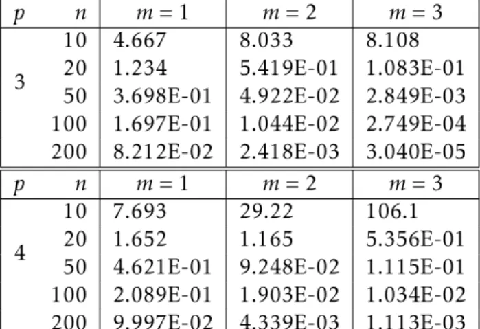
In Table 2.1 are listed the simulated 0.05 cut-offpoints for_T•for some values

ofp,mandn.

(39)

Table 2.1:Cut-off_{points of the 95% confidence set for the regression coe}ffi_{cients matrix}_B_.

n

p= 3

m= 1 m= 3

α= 2 α= 4 α= 4 α= 6

10 6.568 7.433 20.11 29.08

50 5.502E-01 5.581E-01 9.277E-03 9.691E-03 100 2.518E-01 2.542E-01 9.212E-04 9.443E-04 200 1.207E-01 1.208E-01 1.049E-04 1.064E-04

n

p= 4

m= 1 m= 3

α= 2 α= 4 α= 4 α= 6

10 11.08 12.69 239.2 372.7

50 6.884E-01 6.984E-01 3.550E-02 3.697E-02 100 3.108E-01 3.128E-01 3.487E-03 3.564E-03 200 1.487E-01 1.490E-01 3.674E-04 3.723E-04

If instead of testing the regression coefficients matrix_B, someone wants to test

a linear combination of the parameters inB, namely, C=ABwhere A is ak×p

matrix withrank(A) =k≤p andk ≥m, one may define

T_C•=|(AB

•₋_C₎′₍_A₍_XX′₎−1_A′₎−1₍_AB•₋_C₎_|

|(n−p)S•_| ,

which will present a similar distribution to that ofT• in (2.17). If one notes that

(AB•−AB)′_|

˜

Σ−1∼N_mk

0,A(XX′)−1_A′_⊗₍₂_Σ_˜ ₊_Σ₎_,

and that

(AB•−C)′₍_A₍_XX′₎−1

A′)−1₍_AB•₋_C₎_|

˜

Σ−1∼W_m(2Σ˜ +Σ, k), easily realizing that

T_C•|Ω∼st       

m Y

i=1

k−i+ 1

(n−p)−i+ 1Fk,i      

|2Im+Ω|, (2.18)

withF_k,i as independent random variables withF_k−i+1,(n−p)−i+1distribution, them-selves independent ofΩdefined in Theorem2.1.2.

So, if one wants to perform the test

H0:C=C0 versus H1:C,C0,

(40)

simulating the distribution in (2.18). To perform a test forB=B0 one must take

A=I_p,C0=B0 andk =p in (2.18).

A (1−γ) level confidence set forCwill be given by

∆(_C) =_{_C:_T•

C≤ωk,m,n,p;γ}. (2.19)

The inference for the regression coefficients when just a single partially

syn-thetic dataset is released is now made available fulfilling the existing gap and fulfilling the first objective of this work.

This derivation of an exact inference procedure for the singly imputed syn-thetic data generated via PPS, allows the derivation of an exact inferential pro-cedure for multiply imputed synthetic datasets generated via PPS, as shown in subsection2.2.2.

2.2 Multiple imputation: Posterior Predictive

Sampling

In Chapter1, it was referred the inclusion of multiple imputation as a SDC tech-nique for partially synthetic data, treating the values fromsensitivevariables as missing data and replacing these by synthesized values. These values may be generated independently M times via PPS method, which is the most common

method when dealing with missing data.

To specify in detail the PPS method in the MLR model context, let us consider again the model (1.1) withY, X, B, Σ_, ˆBand_Sdefined in that context.

The synthetic data will consist ofM synthetic versions ofYgenerated based on the PPS method.

Let us consider the joint prior distribution

π(B,Σ)_{∝ |}Σ_|−α/2_,

as in subsection2.1.1leading to the same posterior distributions forΣ and_Bas

in (2.1) and (2.2), assuming that n+α > p+m+ 1. Consequently, we draw Σ˜₁

from (2.1) and _B˜₁ _{from (2.2), generating the first synthetic dataset, denoted as} Z1= (z11, . . . ,z1n) wherez1i = (z11i, . . . ,zm1i), are independently distributed as

z1i|B˜1,Σ˜1 ∼Nm

˜

B′₁xi,Σ˜1

, i= 1, . . . , n. (2.20)

Then, we repeat the same procedure in order to generate i.i.d. Z2, . . . ,ZM, by

drawing sequentially Σ˜₂_{, . . . ,}Σ˜_M and _B˜₂_{, . . . ,}_B˜_M, in order to generate i.i.d.

(41)

2 . 2 . M U LT I P L E I M P U TAT I O N : P O S T E R I O R P R E D I C T I V E SA M P L I N G

Z2, . . . ,ZM.

2.2.1 Reiter’s adapted methodology

Before presenting the development of an exact inference procedure, we will present an adaptation of Reiter’s [31] methodology for drawing inference based on multiply synthetic data generated via PPS for a vector valued parameter, to the inference on a matrix value parameter.

In order to be possible to use Reiter’s methodology, developed for a vector of parameters, to estimateB, ap×mdimensional matrix parameter, let us consider vec(B) = (B′₁B′₂ . . . B′_m)′_{, a}_pm_×_{1 vector parameter, where}_B

j(j= 1, . . . , m) denotes

thej-th column ofB.

Based on the original data,vec(ˆB) is an estimator ofvec(B) and its covariance matrix estimator is U=S⊗(XX′₎−1_{, a}

pm×pm matrix. Let Z1, . . . ,ZM be the M

synthetic datasets obtained via PPS. Let vec(B†_j) = vec((XX′₎−1_XZ′

j) and Uj = S†_j ⊗(XX′)−1_{, where} _S†

j = n−1p(Zj −B†

′

j X)(Zj−B†

′

j X)′, for j = 1, . . . , M. Note that

based onZ_j, conditionally on ˆBandS,vec(B†_j) is an UE ofvec(B) andU_j is an UE of its variance. Then the following estimators

vec(B†_M) = 1

M M X

j=1

vec(B†_j), U_M= 1

M M X

j=1

U_j, (2.21)

b_M = 1

M−1

M X

j=1

(vec(B†_j)−vec(B†_M))(vec(B†_j)−vec(B†_M))′ _(2.22)

should be Reiter’s estimators to be used to draw inference aboutB, wherevec(B†_M) is an estimator forvec(B), its variance being estimated byT= _M1b_M+U_M.

Let us consider

T_R,M= (vec(B †

M)−vec(B))′(UM)−1(vec(B †

M)−vec(B))

pm(1 +r) (2.23)

wherer= tr(bMU −1 M)

Mpm . Then following Reiter [31], the distribution ofTR,M is

approx-imated by anF_pm,w(r) distribution where

w(r) = 4 + [pm(M−1)−4]

"

1 +1

r −

2 (M−1)rpm

#2

. (2.24)

(42)

imputation cases, since, in fact, was developed only for multiple imputation and also if one takesM = 1 in the expression ofw(r), above, it becomes meaningless.

Thus the inclusion of the single exact inference method in the previous Section. Second, it is asymptotic in nature and not exact, thus it is not fit for relatively small sample sizes.

With this second problem in mind, follows in the next subsection the develop-ment of an exact inference procedure for the multiply imputed synthetic datasets via PPS.

2.2.2 Exact inference for multiple imputation cases based in

single imputation inference

In order to develop an exact inferential procedure for the multiple imputation case, one first idea could be to obtain the distribution of the mean of theM

indi-vidual estimators ofB,B†_j, and the distribution of the mean of theMindividual

estimators ofΣ,_S†

j, defined in the previous subsection. Unfortunately, this would

be too hard to materialize for the distribution of the mean of the S†_j estimators. Since, to obtain the exact pdf of such an estimator, under the MLR model, one would face the problem of deriving the distribution of the sum of variables that follow Wishart distributions with different parameter matrices.

Therefore, a new approach is presented where each synthetic data is seen as an individual sample.

Let

B†_j = (XX′)−1_XZ′

j (2.25)

and

S†_j = 1

n−p(Zj−B •′

j X)(Zj−B•

′

j X)′ (2.26)

be respectively the estimators of B and Σ based on the _j-th synthetic dataset

(j= 1, . . . , M), which by Lemma1.4.1are jointly sufficient for_BandΣ.

Conditionally on (_B˜_j_,Σ˜_j), for every_j = 1_{, . . . , M},_B†

j will be independent ofS†j

andn(B†₁,S†₁), . . . ,(B†_M,S†_M)owill be jointly sufficient estimators for_BandΣ.

For eachj = 1, . . . , M, individually, one may note that, from Section2.1.1, the

MLE ofBwould beB†_j and ˆS_j =n+α−_np₋−_p2m−2S†_j would be an UE forΣ.

Then, it is proposed the following test statistic

T_M† = M X

j=1

T_j† (2.27)

(43)

2 . 2 . M U LT I P L E I M P U TAT I O N : P O S T E R I O R P R E D I C T I V E SA M P L I N G

with

T_j†= |(B †

j−B)′(XX′)(B†j −B)|

|(n−p)S†_j| .

Let us note that T_M† will be a pivotal quantity due to the fact that, for j =

1, . . . , M, allT_j† are not function of any original data parameter. From Theorem

2.1.2we have that

T_j†|Ω∼st        m Y i=1

     

|2Im+Ω|, j= 1, . . . , M

leading to the conclusion that

T_M†|Ω∼st M X j=1           m Y i=1

     

|2Im+Ω|   ,

whereΩhas the same distribution as_A

1 2 1A−21A

1 2

1, whereA1 ∼Wm(Im, n+α−p−m−1), A2 ∼Wm(Im, n−p) andFi ∼Fp−i+1,n−p−i+1 (i = 1, . . . , m), all independent random

variables.

To test a linear combination of the parameters inB, namely,C=ABwhereA

is ak×pmatrix withrank(A) =k≤pandk≥m, one defines

T_M,† _C= M X

j=1

|(AB†_j −C)′₍_A₍_XX′₎−1_A′₎−1₍_AB† j −C)|

|(n−p)S†_j|

and proceed by noting that

T_M,† _C|_Wst∼

M X j=1           m Y i=1

k−i+ 1 n−p−i+ 1Fk,i

     

|2Im+Ω|  

 (2.28)

withF_k,i ∼F_k−i+1,n−p−i+1, all independent variables, themselves independent ofΩ, which is defined as above.

In order to test

H0:C=C0 versus H1:C,C0,

we reject H0 whenever T_M,† C0 exceeds ψM,k,m,n,p;γ, where ψM,k,m,n,p;γ satisfies (1−γ) =Pr(T_M,† _C₀ ≤ψ_M,k,m,n,p;γ) whenH0 is true, where the value ofψM,k,m,n,p;γ