Recurrent gaussian processes and robust dynamical modeling

CENTRO DE TECNOLOGIA

DEPARTAMENTO DE ENGENHARIA DE TELEINFORM ´ATICA

PROGRAMA DE P ´OS-GRADUA ¸C ˜AO EM ENGENHARIA DE TELEINFORM ´ATICA

DOUTORADO EM ENGENHARIA DE TELEINFORM ´ATICA

C´ESAR LINCOLN CAVALCANTE MATTOS

RECURRENT GAUSSIAN PROCESSES AND ROBUST DYNAMICAL MODELING

RECURRENT GAUSSIAN PROCESSES AND ROBUST DYNAMICAL MODELING

Tese apresentada ao Curso de Doutorado em Engenharia de Teleinform´atica do Programa de P´os-Gradua¸c˜ao em Engenharia de Teleinform´atica do Centro de Tecnologia da Universidade Federal do Cear´a, como requisito parcial `a obten¸c˜ao do t´ıtulo de doutor em Engenharia de Teleinform´atica.

´

Area de Concentra¸c˜ao: Sinais e sistemas

Orientador: Prof. Dr. Guilherme de Alencar Barreto

Biblioteca Universitária

Gerada automaticamente pelo módulo Catalog, mediante os dados fornecidos pelo(a) autor(a)

M39r Mattos, César Lincoln.

Recurrent Gaussian Processes and Robust Dynamical Modeling / César Lincoln Mattos. – 2017. 189 f. : il. color.

Tese (doutorado) – Universidade Federal do Ceará, Centro de Tecnologia, Programa de Pós-Graduação em Engenharia de Teleinformática, Fortaleza, 2017.

Orientação: Prof. Dr. Guilherme de Alencar Barreto.

1. Processos Gaussianos. 2. Modelagem dinâmica. 3. Identificação de sistemas não-lineares. 4. Aprendizagem robusta. 5. Aprendizagem estocástica. I. Título.

RECURRENT GAUSSIAN PROCESSES AND ROBUST DYNAMICAL MODELING

A thesis presented to the PhD course in Teleinformatics Engineering of the Graduate Program on Teleinformatics Engineering of the Center of Technology at Federal University of Cear´a in fulfillment of the the requirement for the degree of Doctor of Philosophy in Teleinformatics Engineering.

Area of Concentration: Signals and systems

Approved on: August 25, 2017

EXAMINING COMMITTEE

Prof. Dr. Guilherme de Alencar Barreto (Supervisor)

Universidade Federal do Cear´a (UFC)

Prof. Dr. Antˆonio Marcos Nogueira Lima Universidade Federal de Campina Grande

(UFCG)

Prof. Dr. Oswaldo Luiz do Valle Costa Universidade de S˜ao Paulo (USP)

I would like to thank my supervisor, Prof. Guilherme de Alencar Barreto, for his long-time support, partnership and academic guidance. Guilherme knows a fine balance between a focused supervision and the freedom to explore and experiment. His patience, encouragement and dedication throughout all the PhD journey were invaluable.

I thank my many friends in the PPGETI, for all the intra and extra campus conversations about the most diverse topics. You were very important to proportionate a suitable environment for all this period. I specially thank Jos´e Daniel Alencar and Amauri Holanda, with whom I had many valuable discussions.

I am very grateful to Prof. Neil Lawrence, for kindly receiving me in his research group in the University of Sheffield. Neil has been a great intellectual inspiration and provided a significant boost to my studies. The way he works in his group and handles machine learning research will always have an influence on me.

I was very lucky to be around Neil’s ML group in SITraN for six months. I learned so much from the incredible people I met there. All the experiences we shared were critical for my adaptation and will be treasured. Thanks a lot, everyone! A special thanks to my co-authors, Andreas Damianou and Zhenwen Dai, who dedicated a lot of time to help me with my research (and are great guys!).

I acknowledge the financial support of FUNCAP (for my PhD scholarship) and CAPES (for my time abroad via the PDSE program).

not possession but the act of getting there, which grants the greatest enjoyment.”

O estudo de sistemas dinˆamicos encontra-se disseminado em v´arias ´areas do conhecimento. Dados sequenciais s˜ao gerados constantemente por diversos fenˆomenos, a maioria deles n˜ao pass´ıveis de serem explicados por equa¸c˜oes derivadas de leis f´ısicas e estruturas conhecidas. Nesse contexto, esta tese tem como objetivo abordar a tarefa de identifica¸c˜ao de sistemas n˜ao lineares, por meio da qual s˜ao obtidos modelos diretamente a partir de observa¸c˜oes sequenciais. Mais especificamente, n´os abordamos cen´arios desafiadores, tais como o aprendizado de rela¸c˜oes temporais a partir de dados ruidosos, dados contendo valores discrepantes (outliers) e grandes conjuntos de dados. Na interface entre estat´ısticas, ciˆencia da computa¸c˜ao, an´alise de dados e engenharia encontra-se a comunidade de aprendizagem de m´aquina, que fornece ferramentas poderosas para encontrar padr˜oes a partir de dados e fazer previs˜oes. Nesse sentido, seguimos m´etodos baseados em Processos Gaussianos (PGs), uma abordagem probabil´ıstica pr´atica para a aprendizagem de m´aquinas de kernel.

A partir de avan¸cos recentes em modelagem geral baseada em PGs, introduzimos novas contribui¸c˜oes para o exerc´ıcio de modelagem dinˆamica. Desse modo, propomos a nova fam´ılia de modelos de Processos Gaussianos Recorrentes (RGPs, da sigla em inglˆes) e estendemos seu conceito para lidar com requisitos de robustez a outliers e aprendizagem estoc´astica escal´avel. A estrutura hier´arquica e latente (n˜ao-observada) desses modelos imp˜oe express˜oes n˜ao-anal´ıticas, que s˜ao resolvidas com a deriva¸c˜ao de novos algoritmos variacionais para realizar inferˆencia determinista aproximada como um problema de otimiza¸c˜ao. As solu¸c˜oes apresentadas permitem a propaga¸c˜ao da incerteza tanto no treinamento quanto no teste, com foco em realizar simula¸c˜ao livre. N´os avaliamos em detalhe os m´etodos propostos com benchmarks artificiais e reais da ´area de identifica¸c˜ao de sistemas, assim como outras tarefas envolvendo dados dinˆamicos. Os resultados obtidos indicam que nossas proposi¸c˜oes s˜ao competitivas quando comparadas a modelos dispon´ıveis na literatura, mesmo nos cen´arios que apresentam as complica¸c˜oes mencionadas, e que a modelagem dinˆamica baseada em PGs ´e uma ´area de pesquisa promissora.

The study of dynamical systems is widespread across several areas of knowledge. Sequential data is generated constantly by different phenomena, most of them that we cannot explain by equations derived from known physical laws and structures. In such context, this thesis aims to tackle the task of nonlinear system identification, which builds models directly from sequential measurements. More specifically, we approach challenging scenarios, such as learning temporal relations from noisy data, data containing discrepant values (outliers) and large datasets. In the interface between statistics, computer science, data analysis and engineering lies the machine learning community, which brings powerful tools to find patterns from data and make predictions. In that sense, we follow methods based on Gaussian Processes (GP), a principled, practical, probabilistic approach to learning in kernel machines. We aim to exploit recent advances in general GP modeling to bring new contributions to the dynamical modeling exercise. Thus, we propose the novel family of Recurrent Gaussian Processes (RGPs) models and extend their concept to handle outlier-robust requirements and scalable stochastic learning. The hierarchical latent (non-observed) structure of those models impose intractabilities in the form of non-analytical expressions, which are handled with the derivation of new variational algorithms to perform approximate deterministic inference as an optimization problem. The presented solutions enable uncertainty propagation on both training and testing, with focus on free simulation. We comprehensively evaluate the introduced methods with both artificial and real system identification benchmarks, as well as other related dynamical settings. The obtained results indicate that our propositions are competitive when compared to models available in the literature within the aforementioned complicated setups and that GP-based dynamical modeling is a promising area of research.

Figure 1 – Block diagrams of common evaluation methodologies for system

identi-fication. . . 25

Figure 2 – Examples of GP samples with different covariance functions. . . 34

Figure 3 – Graphical model detailing the relations between the variables in a standard GP model. . . 36

Figure 4 – Samples from the GP model before and after the observations. . . 38

Figure 5 – Illustration of the Bayesian model selection procedure. . . 39

Figure 6 – Simplified graphical models for the standard and augmented sparse GPs. 47 Figure 7 – Comparison of standard GP and variational sparse GP regression. . . . 48

Figure 8 – Simplified graphical model for the GP-LVM. . . 49

Figure 9 – Graphical model for the Deep GP. . . 51

Figure 10 – Graphical model for the GP-NARX. . . 56

Figure 11 – Graphical model for the GP-SSM. . . 59

Figure 12 – RGP graphical model with H hidden layers. . . 63

Figure 13 – Detailing of a single recurrent transition layer h,1_≤h_≤H, of the RGP model. . . 63

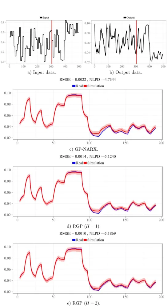
Figure 14 – Example of system identification with the RGP model. . . 81

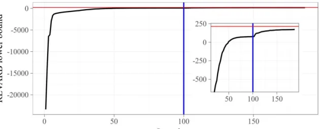
Figure 15 – Convergence curve of the REVARB lower bound during the training step of the RGP model withH=2hidden layers on theExample dataset using the BFGS algorithm. . . 82

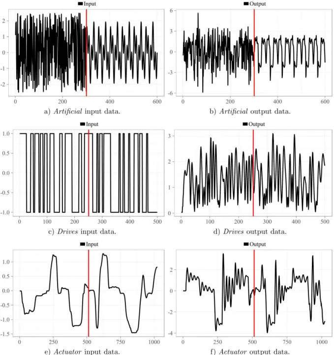
Figure 16 – Datasets considered for the nonlinear system identification task. . . 84

Figure 17 – Free simulation on nonlinear system identification test data. . . 86

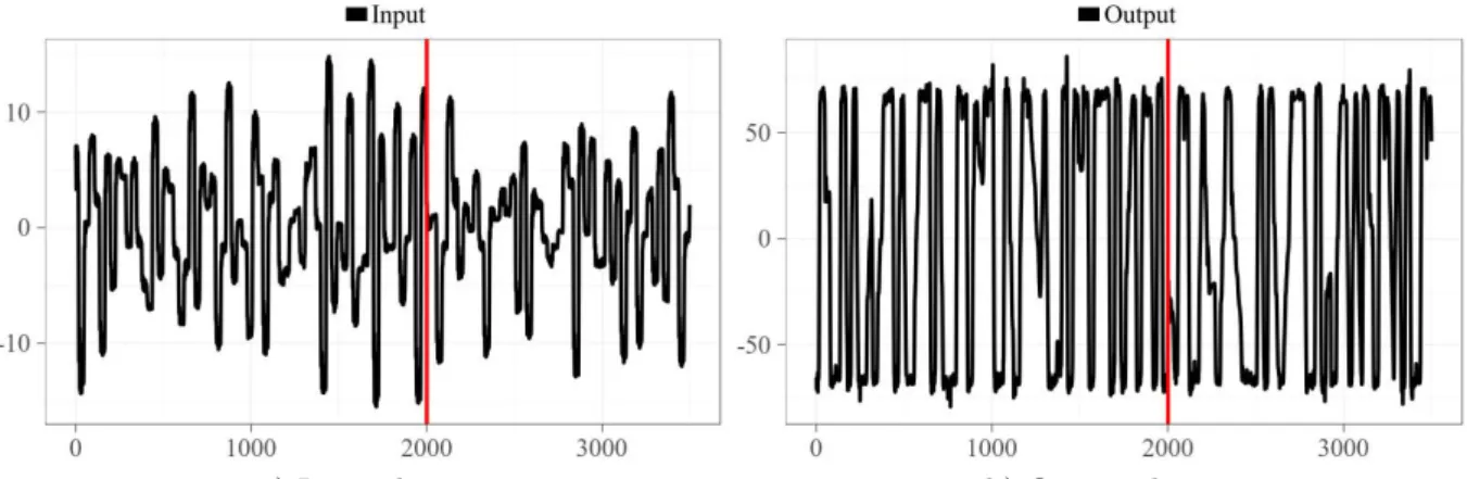
Figure 18 – Input and output series for the Damper dataset. . . 87

Figure 19 – Free simulation on test data with the 2-hidden layer RGP model after estimation on theDamper dataset. . . 88

Figure 20 – Input and output series for the Cascaded Tanks dataset. . . 89

Figure 21 – Free simulation on test data with the RGP model after estimation on the Cascaded Tanks dataset. . . 90

for the average velocity. . . 93 Figure 24 – Comparison between the Gaussian likelihood and heavy-tailed

distribu-tions. . . 98 Figure 25 – Effect of outliers on both standard and robust GP regression models. . 99 Figure 26 – Graphical models for some of the robust GP-based approaches considered

for dynamical modeling in this chapter. . . 113 Figure 27 – Line charts for the RMSE values related to the free simulation on test

data with different levels of contamination by outliers. The correspon-dent bar plots indicate the percentage of outliers detected by the robust models using the variational framework. . . 122 Figure 28 – Example of the robust filtering property of the GP-RLARX model. . . 123 Figure 29 – Free simulation on test data after estimation on the pH train dataset

without and with outliers. . . 125 Figure 30 – Outlier detection by the RGP-tmodel with 2 hidden layers and

REVARB-t inference for thepH estimation data . . . 125 Figure 31 – Free simulation on test data after estimation on the Heat Exchanger

train dataset without and with outliers. . . 127 Figure 32 – Outlier detection by the RGP-t model with 2 hidden layers for the Heat

Exchanger estimation data . . . 128 Figure 33 – Diagram for the MLP and RNN-based recognition models of the Global

S-REVARB framework in a RGP model withH recurrent layers. . . 140 Figure 34 – Convergence curves of the S-REVARB lower bound with H=2 hidden

layers, in both Local and Global variants, during the training step on the Damper dataset using the Adam stochastic gradient algorithm. . . 147 Figure 35 – Comparison between the absolute test errors obtained by the Global

S-REVARB and the RNN on the Silverbox dataset, both with one hidden layer. . . 151 Figure 36 – Comparison between the absolute test errors obtained by the Global

Table 1 – List of regressors used by common model structures with external dynamics. 55 Table 2 – Summary of RMSE values for the free simulation results on system

identification test data. . . 85 Table 3 – RMSE and NLPD values for the free simulation results on the Damper

dataset. . . 87 Table 4 – Free simulation results on the Cascaded Tanks dataset. . . 90 Table 5 – Results for free simulation on the Mackey-Glass time series. . . 91 Table 6 – Summary of RMSE values for the free simulation results on human

motion test data. . . 92 Table 7 – Details of the five artificial datasets used in the computational

experi-ments related to the task of robust system identification. . . 104 Table 8 – Summary of test free simulation RMSE values in scenarios with different

contamination rates by outliers in the estimation data. . . 105 Table 9 – Details of the sixth artificial dataset used in the robust computational

experiments. . . 121 Table 10 – RMSE and NLPD results for free simulation on test data after estimation

on the pH dataset without and with outliers. . . 124 Table 11 – RMSE and NLPD results for free simulation on test data after estimation

on the Heat Exchanger dataset without and with outliers. . . 127 Table 12 – Comparison of computational and memory requirements of some

GP-based dynamical models. . . 137 Table 13 – RMSE and NLPD values for the free simulation results of the S-REVARB

framework on the Damper dataset. . . 146 Table 14 – Summary of results for the free simulation on test data after estimation

from large dynamical datasets. . . 150 Table 15 – Comparison of the number of adjustable parameters (RNNs) or

hyper-parameters and variational hyper-parameters (S-REVARB variants) in the experiments with the Wiener-Hammerstein benchmark (N=95,000). . 150 Table 16 – Summary of features presented by some of the different dynamical

Algorithm 1 – Standard GP modeling for regression. . . 40

Algorithm 2 – REVARB for dynamical modeling with the RGP model. . . 76

Algorithm 3 – GP-RLARX for outlier-robust dynamical modeling. . . 111 Algorithm 4 – REVARB-t for outlier-robust dynamical modeling with the RGP-t

model. . . 120

ARD Automatic Relevance Determination

BFGS Broyden-Fletcher-Goldfarb-Shanno (algorithm) EM Expectation Maximization

EP Expectation Propagation ESGP Echo State GP

ESN Echo State Network GP Gaussian Process

GP-LEP GP model with Laplace likelihood and EP inference GP-NARX GP model with NARX structure

GP-RLARX Robust GP Latent Autoregressive Model GP-SSM GP model with SSM structure

GP-tVB GP model with Student-t likelihood and variational inference GPDM Gaussian Process Dynamical Model

GP-LVM Gaussian Process Latent Variable Model KL Kullback-Leibler (divergence)

KLMS Kernel Least Mean Squares KRLS Kernel Recursive Least-Squares LSTM Long Short-Term Memory MAP Maximum a Posteriori MCMC Markov Chain Monte Carlo

MIMO Multiple-Input and Multiple-Output ML Maximum Likelihood

MLP Multilayer Perceptron MLP-NARX MLP with NARX structure NAR Nonlinear Autoregressive

NARMAX Nonlinear Autoregressive Moving Average with eXogenous inputs NARX Nonlinear Autoregressive with eXogenous inputs

NFIR Nonlinear Finite Impulse Response NLPD Negative Log-Predictive Density NN Neural Network

PAM Partition Around Medoids PCA Principal Component Analysis RBF Radial Basis Function

ReLu Rectifier Linear Unit

REVARB REcurrent VARiational Bayes REVARB-t REVARB with Student-t likelihood RGP Recurrent Gaussian Process

RGP-t RGP with Student-t likelihood RKHS Reproducing Kernel Hilbert Spaces RMSE Root Mean Square Error

RNN Recurrent Neural Network SISO Single-Input and Single-Output

SISOG System Identification using Sparse Online GP SMC Sequential Monte Carlo

SNR Signal to Noise Ratio S-REVARB Stochastic REVARB SSM State-Space Model

SVI Stochastic Variational Inference SVI-GP SVI for sparse GP models SVM Support Vector Machines

TBPTT Truncated Backpropagation Through Time VB Variational Bayes

hip(·) Expectation with respect to the distribution p(·)

D Input dimension

E_{{·} Mean of the random variable in the argument}

ε_i(h) Noise variable related to the i-th instant of theh-th layer

ζζζ(_mh) j-th pseudo-input of the h-th layer

f(_·) Unknown (possibly) nonlinear function

fi Latent function value in the i-th instant

f_∗ Latent function value related to a test input

H Number of hidden layers

III Identity matrix

k(_·,_·) Covariance (or kernel) function

K K

Kf z Covariance (or kernel) matrix between the vectors fff and zzz

K K

Kf Covariance (or kernel) matrix related to the vector fff

KL(_·||·) Kullback-Leibler divergence

L Order of the lagged latent dynamical variables

Lu Order of the lagged exogenous inputs

Ly Order of the lagged outputs

λ_i(h) Variational variance related to the i-th dynamical latent variable of the

h-th layer

log Natural logarithm operator

M Number of pseudo-inputs

µ_i(h) Variational mean related to the i-th dynamical latent variable of the

h-th layer

N Number of estimation (or training) samples

p(_·) Probability density function

q(_·) Variational distribution

Tr Trace operator

θ θ

θ Vector of parameters or hyperparameters

τi Precision (inverse variance) related to the i-th observation

ui Exogenous system input in the i-th instant

V_{{·} Variance of the random variable in the argument}

wd d-th inverse lengthscale hyperparameter

x(_ih) Dynamical latent variable in thei-th instant of the h-th layer

¯

xxx(_ih) Latent regressor vector in the i-th instant of theh-th layer

ˆ

xxx(_ih) Input vector in thei-th instant of the h-th layer

xxx_∗ Test input vector

ˆ

X X

X(h) Stack of all the vectors xxxˆ(_ih)

yi System observed output in the i-th instant

y_∗ System observed output related to a test output

1 INTRODUCTION . . . 20

1.1 Objectives . . . 23

1.2 System Identification . . . 23

1.3 Probabilistic Reasoning . . . 25

1.4 A Word About Notation and Nomenclature . . . 26

1.5 List of Publications . . . 28

1.6 Organization of the Thesis . . . 29

2 THE GAUSSIAN PROCESS MODELING FRAMEWORK . 31 2.1 Multivariate Gaussian Distribution: Two Important Properties 31 2.2 GP Prior over Functions . . . 32

2.3 Inference from Noisy Observations . . . 34

2.4 Bayesian Model Selection . . . 37

2.5 From Feature Spaces to GPs . . . 41

2.6 Sparse GP Models . . . 43

2.6.1 The Variational Sparse GP Framework . . . 43

2.7 Unsupervised GP Modeling and Uncertain Inputs . . . 49

2.8 Hierarchical and Deep Gaussian Processes . . . 51

2.9 Discussion . . . 53

3 DYNAMICAL MODELING AND RECURRENT GAUSSIAN PROCESSES MODELS . . . 54

3.1 Dynamical Modeling with GPs . . . 54

3.1.1 GP Models with External Dynamics . . . 55

3.1.2 GP Models with Internal Dynamics . . . 57

3.2 Recurrent GPs . . . 61

3.3 REVARB: REcurrent VARiational Bayes . . . 64

3.3.1 Making Predictions with the REVARB Framework . . . 69

3.3.2 Sequential RNN-based Recognition Model . . . 72

3.3.3 Multiple Inputs and Multiple Outputs . . . 73

3.3.4 Implementation Details . . . 75

3.4 Experiments . . . 79

3.4.2.1 Magneto-Rheological Fluid Damper Data. . . 85

3.4.2.2 Cascaded Tanks Data . . . 88

3.4.3 Time Series Simulation. . . 89

3.4.4 Human Motion Modeling. . . 92

3.4.5 Avatar Control . . . 93

3.5 Discussion . . . 93

4 ROBUST BAYESIAN MODELING WITH GP MODELS . . 96

4.1 Robust GP Model with Non-Gaussian Likelihood . . . 97

4.1.1 The GP-tVB Model . . . 100

4.1.2 The GP-LEP Model . . . 102

4.1.3 Evaluation of GP-tVB and GP-LEP for Robust System Iden-tification . . . 103

4.2 GP-RLARX: Robust GP Latent Autoregressive Model . . . . 106

4.3 The RGP-t Model . . . 111

4.4 The REVARB-t Framework . . . 114

4.4.1 Making Predictions with the REVARB-t Framework . . . 118

4.5 Experiments . . . 119

4.5.1 Artificial Benchmarks . . . 120

4.5.2 pH Data . . . 124

4.5.3 Heat Exchanger Data . . . 126

4.6 Discussion . . . 128

5 GP MODELS FOR STOCHASTIC DYNAMICAL MODELING130 5.1 Stochastic Optimization . . . 131

5.2 Stochastic Variational Inference with GP Models . . . 131

5.3 S-REVARB: A Stochastic REVARB Framework . . . 135

5.3.1 Local S-REVARB: Recurrent SVI . . . 138

5.3.2 Global REVARB: Sequential Recognition Models for S-REVARB . . . 139

5.3.3 Making Predictions with the S-REVARB Framework . . . 141

5.3.4 Implementation Details . . . 143

5.4.2 Stochastic System Identification with Large Datasets . . . 148

5.5 Discussion . . . 152

6 CONCLUSIONS . . . 154

6.1 Future Work . . . 155

BIBLIOGRAPHY . . . 158

APPENDIX . . . 175

1 INTRODUCTION

“The most important questions of life are indeed, for the most part, only problems of probability.”

(Pierre-Simon Laplace)

The contemporary world is immersed in a great variety of systems and sub-systems with intricate interactions between themselves and with our society. Some of those systems are related to fixed input-output mappings and, therefore, only the current interactions affect their operation. Those are labeled as static systems. However, the class of dynamical systems do not present those properties and require distinct study strategies.

The concept of a dynamical system defines a process whose state presents a temporal dependence. In other words, the output of the system depends not only on the current external inputs but also their previous values. In many cases the external stimuli is easy to define, for instance, the opening of a valve in a hydraulic actuator or the wind speed in a wind turbine. Alternatively, if the external signals that excite the system are not observed, its measured outputs are usually called a times series (LJUNG, 1999). Those definitions may be used to describe phenomena of several different fields, such as engineering, physics, chemistry, biology, finance and sociology (CHUESHOV, 2002). Moreover, it is important to note that, ultimately, all real systems are dynamical, even though for some of them the static analysis is sufficient (AGUIRRE, 2007).

The analysis of a dynamical system demands that its behavior must be ex-plained by a mathematical model, which can be obtained theoretically or empirically. The theoretical methodology is based on findings supported by equations relating pa-rameters from a known structure, determined by underlying physical laws. On the other hand, the experimental approach, named identification, seeks an appropriate model from measurements and a priori knowledge, possibly acquired from past experiments (ISER-MANN; M ¨UNCHHOF, 2011). The latter, which avoids the limitations and problem-specific complexities of the purely theoretical approach, is the main application subject of this work.

usually involve much more complex analyses, provided the wide class of possible model nonlinearities (BILLINGS, 2013). Since the quality of the model is frequently the bottleneck of the final problem solution (NELLES, 2013), complications such as noisy data and the presence of discrepant observations in the form of outliers must be carefully considered. Moreover, modern systems have generated increasingly larger datasets, a feature which by itself provides algorithmic and computational demands.

As described so far, the system identification exercise seems a perfect candidate to be tackled by the machine learning community, a field closely related to statistics and at the intersection of computer science, data analysis and engineering. The goal of machine learning is to apply methods that can detect patterns in data, make predictions and aid decision making (MURPHY, 2012). As opposed to other common machine learning applications, such as standard continuous regression (static mapping) and classification (mapping to discrete classes), we are interested in working with sequential records. Thus,

all the models presented in this work can be viewed as machine learning efforts tailored to handle dynamical data. It is worth mentioning the recent preprint work by Pillonetto (2016), who analyzes general connections between the fields of system identification and

machine learning, with focus on the shared problem of learning from examples.

In this thesis we mainly follow the Bayesian point of view, where the model accounts for the uncertainty in the noisy data and in the learned dynamics (PETERKA, 1981). More specifically, we apply Gaussian Processes (GP) models, a principled, practical, probabilistic approach to learning in kernel machines (RASMUSSEN; WILLIAMS, 2006). Differently from modeling approaches that aim to fit a parametrized structure to a system’s inputs and outputs, a GP model directly describes the probabilistic relations between the output data with respect to the inputs (KOCIJAN, 2016). Thus, GP models have been widely applied to the so called “black box” approach1 to system modeling (AˇZMAN; KOCIJAN, 2011). The probabilistic information obtained a posteriori from GP models, i.e., after training using observed data, has made them an attractive stochastic tool to applications in control and system identification in general (KOCIJAN et al., 2005).

The Bayesian nature of GP-based models considers the uncertainty inherited from the quality of the available data and the modeling assumptions, which enables a clear probabilistic interpretation of its predictions. Thus, an immediate advantage of the GP

1

framework over other regression methods, like Neural Networks (NNs) or Support Vector Machines (SVMs), is that its outputs are distributions, i.e., instead of point estimates, each prediction is given by a fully defined probability distribution. Therefore, it explicitly indicates its uncertainty due to limited information about the process that generated the observed data and enables error bars in the predictions, a valuable feature in many applications, such as control and optimization. Gregorˇciˇc and Lightbody (2008) present some more advantages of GPs over other learning methods, such as the reduced number of hyperparameters, less susceptibility to the so called “curse of dimensionality”2 and the more transparent analysis of the obtained results due to the uncertainty they are able to express.

Taking advantage of the aforementioned features, the authors have explored diverse applications of GP-based dynamical models, such as nonlinear signal processing (P´EREZ-CRUZ et al., 2013), human motion modeling (EK et al., 2007; WANG et al.,

2008; JIANG; SAXENA, 2014), speech representation and synthesis (HENTER et al., 2012; KORIYAMAet al., 2014), fault detection (JURICIC; KOCIJAN, 2006; OSBORNE et al., 2012) and model-based control (KOCIJAN et al., 2004; LIKAR; KOCIJAN, 2007; KO et al., 2007; DEISENROTH; RASMUSSEN, 2011; ROCHA et al., 2016; KLENSKEet al., 2016; VINOGRADSKAet al., 2016).

There is also a vast body of theses with diverse contributions to the use of GP-based methods to dynamical modeling and more in-depth theoretical and empirical analyses, such as GP with noisy inputs and derivative observations (GIRARD, 2004), multiple GPs and state-space time series models (NEO, 2008), implementation and application to engineering systems (THOMPSON, 2009), nonlinear filtering and change-point detection (TURNER, 2012). Recently, work in this topic has been even more active, with several authors proposing more flexible model structures, powerful learning algorithms and tackling task-specific issues in their doctoral researches (MCHUTCHON, 2014; FRIGOLA-ALCADE, 2015; DAMIANOU, 2015; SVENSSON, 2016; BIJL, 2016).

The present PhD work builds upon such rich literature on dynamical GP-based models in order to revisit the problem of nonlinear system identification. We aim to exploit recent advances in general GP modeling to bring new contributions to the field, as detailed in our objectives, listed as follows.

2

1.1 Objectives

The main objective of this thesis consists in elaborating and evaluating GP-based formulations capable of modeling dynamical systems in challenging scenarios, such as when facing noisy datasets, data containing outliers or very large training sets.

The specific objectives of our work are listed below:

1. To propose a novel GP-based model specifically designed to learn dynamics from sequential data, with the focus on accounting for data and model uncertainties over both training and testing;

2. To propose novel GP-based models to tackle the problem of learning dynamics from data containing non-Gaussian noise in the form of outliers;

3. To propose a novel inference methodology to enable stochastic training of dynamical GP models with large datasets;

4. To evaluate all the proposed models in their specific tasks by performing free simulation on unseen data, as described in the next section.

1.2 System Identification

The system identification task, i.e., the process of obtaining a model only from a system’s inputs and outputs, can be summarized by the following major steps (LJUNG, 1999):

1. Collect data: Via specifically designed experiments, data is recorded from a real system, where the user chooses the measured signals, sampling rates and the inputs to excite its dynamics, aiming for the most informative records possible. Note however that sometimes one has to build a model only from the data obtained during the system normal operation.

2. Determine model structure: A sufficiently general class of models is chosen in order to constrain the search for a good model to explain the analyzed phenomenon. Such structure may contain adjustable parameters to enable variations in its behavior. 3. Perform model selection: The identification step, where the collected data is

used to estimate unknown parameters, usually by assessing how well the model is able to reproduce the collected data, as quantified by a given rule.

with the chosen model are acceptable, preferably using data similar but not equal to the records used in the model selection phase, in order to evaluate the model generalization capability. The validation metric should be chosen accordingly the final model application.

As many engineering procedures, the previous steps may be repeated until one is satisfied with the obtained results, revising each step after analyzing encountered issues. In the present thesis we are mostly interested in the latter three steps, since the data collection step is considered to have been already done. We refer the readers to Ljung (1999), Zhu (2001), Aguirre (2007), Isermann and M¨unchhof (2011) to learn more about

such data recording step, also called experiment design.

Regarding Step 4 of the aforementioned system identification methodology, i.e., where the selected dynamical model is used to perform predictions using separate test data, two common evaluation approaches are described below (NELLES, 2013):

One-step-ahead prediction The next prediction is based on previous test inputs and test observed outputs until the current instant, in a feedforward fashion. Typical applications include weather and stock market forecasting, where measures are readily available and applied especially for short-term prediction.

Free simulation Predictions are made only from past immediate test inputs and predic-tions, without using past test observapredic-tions, following a recurrent structure. It is also called infinite step ahead prediction, model predicted output or simply simulation. Such procedure is necessary when the model will be used to replace the original system, for instance, to experiment with different inputs or as a way to diagnose a real process.

Fig. 1 illustrates the difference between the evaluation strategies described above, considering an autoregressive set-up. The external input of the i-th iteration is denoted as ui, while the noiseless system output, noisy measurement (corrupted by the

disturbance ε_i(y)) and model prediction are respectively fi, yi and f˜i. The z−1 blocks

System +

ε_i(y)

Model

z−1

z−1

.. .

z−1

z−1

z−1

.. .

z−1

ui fi yi

˜ fi

System +

ε_i(y)

Model

z−1

z−1

.. .

z−1

z−1

z−1

.. .

z−1

ui fi yi

˜ fi

(a) One-step ahead prediction. (b) Free simulation.

Figure 1 – Block diagrams of common evaluation methodologies for system identification. The z−1 blocks indicate unit delays. The red lines highlight the difference between both approaches. Note that the left diagram presents a feedforward configuration, as opposed to the diagram in the right, which is recurrent.

1.3 Probabilistic Reasoning

We mostly adopt in this thesis a probabilistic approach to modeling3_{. Its main} ingredient is the account for uncertainty, which comes from noisy observations, finite data and our limited understanding about the analyzed phenomenon (BISHOP, 2006; BARBER, 2012). Those characteristics are intrinsic to machine learning in general, which turns probability an important tool for the area. Although in the present thesis we are not directly interested in discussing about the basic meanings and interpretations about the very much vague concept of probability, it is worth mentioning some of the predominant views.

One possible view is to consider probability as being the long run frequency of events, i.e., the probability of a certain event would be given by its frequency in the limit of a very large number of trials (MURPHY, 2012). That is called the frequentist interpretation or simply frequentism.

3

Another view treats probability as the quantification of our belief about some-thing. In this approach, the Bayesian view, the uncertainty of an event is related to the degree of information we have about it (JEFFREYS, 1998; JAYNES, 2003; COX, 2006). As already mentioned, this is the approach followed by the present work.

The fundamental step in Bayesian modeling is to performreasoning, orinference, i.e., to learn a probability model given a dataset and output probability distributions on unobserved quantities, such as components of the model itself or predictions for new observations (GELMAN et al., 2014a).

From a methodological point of view, it is interesting to separate the concepts of model and learning algorithm. While the first is the mathematical way of representing knowledge, for instance, in a probabilistic way, the latter is the procedure in which we perform inference with our model. Such separation is important to enable model and learning algorithm analyses and improvements independently of each other, as well as to apply different inference methods to the same model in distinct applications (KOLLER; FRIEDMAN, 2009).

As we have already declared, in this thesis our main interest lies in the GP modeling approach, which is first of all a Bayesian nonparametric framework. The first term of such label indicates, as previously discussed, that it treats the uncertainty of the data and the model itself by probability means. The second term indicates the absence of a finite set of parameters, i.e., the knowledge captured by the model is not concentrated in a fixed set of tunable weights, such as in neural networks or models with weighted basis functions4. Furthermore, the complexity of a GP model grows with the amount of data made available. In other words, instead of a rigid prespecified structure, the model allows for the data to “speak by itself”.

1.4 A Word About Notation and Nomenclature

We have tried to maintain a certain degree of formalism in the mathematical descriptions of the current work, while constantly reminding ourselves of our practical goals over pure analytical derivations. Nevertheless, we could not avoid the common problem of choosing and keeping a comprehensive mathematical notation. In order to avoid confusion,

we refer the readers to the List of Symbols at the beginning of this document, which is complemented by the additional conventions below, adopted throughout this thesis.

• We follow a notation for random variables common in the the probabilistic modeling literature, used for instance by Neal (1994), S¨arkk¨a (2013), Gelman et al. (2014a). Thus, a vector fff with a multivariate Gaussian distribution defined by its mean µµµ

and covariance matrix KKK is denoted as fff _∼N _{(µµµ,KKK) or equivalently via its explicit}

density function p(fff) =N _{(fff|µµµ,KKK). Note that, in the latter, the symbol ‘|’ is used}

to highlight the random variable associated with the distribution and separate it from other quantities.

• Although probability density functions are written using p(_·), we use the notation

q(_·) to denote a variational distribution, i.e., a parametrized simpler function used to approximate a more complex density. A factorized variational distribution of multiple variables, e.g., fff and xxx, is sometimes compactly written as Q=q(fff)q(xxx).

• In probabilistic models we frequently have to marginalize random variables in joint or conditional distributions. Such operation consists in integrating out a variable from a given distribution considering all the possible values it can assume. For instance, to marginalize the variable fff from the joint distribution p(yyy,fff), we have to solve the integral p(yyy) =R₋∞∞p(yyy,fff)dfff.

In this thesis we rewrite the former integral in an equivalent but more compact way: R_fff p(yyy,fff), where the subindex in the integral symbol indicates the integrated variables over their respective domains, with the operation considering all the possible values it can take. This approach, adopted for instance by Barber (2012), will allow us to write long expressions avoiding notation clutter.

1.5 List of Publications

The following works were developed during the course of the PhD period. The works marked with a “*” are the ones more directly related to the main subjects of the present thesis, but all of them were relevant to the overall academic formation.

1. C´esar L. C. Mattos; Jos´e D. A. Santos & Guilherme A. Barreto (2014). Classifi-ca¸c˜ao de padr˜oes robusta com redes Adaline modificadas, XI Encontro Nacional de Inteligˆencia Artificial e Computacional, ENIAC 2014.

2. Jos´e D. A. Santos; C´esar L. C. Mattos & Guilherme A. Barreto (2014). A Novel Recursive Kernel-Based Algorithm for Robust Pattern Classification, 15th International Conference on Intelligent Data Engineering and Automated Learning, IDEAL 2014.

3. C´esar L. C. Mattos; Jos´e D. A. Santos & Guilherme A. Barreto (2014). Improved Adaline Networks for Robust Pattern Classification, 24th International Conference on Artificial Neural Networks, ICANN 2014.

4. *C´esar L. C. Mattos; Jos´e D. A. Santos & Guilherme A. Barreto (2015). Uma avalia¸c˜ao emp´ırica de modelos de processos Gaussianos para identifica¸c˜ao robusta de sistemas dinˆamicos, XII Simp´osio Nacional de Automa¸c˜ao Inteligente, SBAI 2015. 5. Jos´e D. A. Santos; C´esar L. C. Mattos& Guilherme A. Barreto (2015).

Perfor-mance Evaluation of Least Squares SVR in Robust Dynamical System Identification, Lecture Notes in Computer Science, vol. 9095, pages 422-435.

6. *C´esar L. C. Mattos; Jos´e D. A. Santos & Guilherme A. Barreto (2015). An Empirical Evaluation of Robust Gaussian Process Models for System Identification, Lecture Notes in Computer Science, vol. 9375, pages 172-180.

7. *C´esar L. C. Mattos; Andreas Damianou; Guilherme A. Barreto & Neil D. Lawrence (2016). Latent Autoregressive Gaussian Processes Models for Robust System Identification, 11th IFAC Symposium on Dynamics and Control of Process Systems DYCOPS-CAB 2016.

8. *C´esar L. C. Mattos; Zhenwen Dai; Andreas Damianou; Jeremy Forth; Guilherme A. Barreto & Neil D. Lawrence (2016). Recurrent Gaussian Processes, International Conference on Learning Representations, ICLR 2016.

Performance Comparison, 14th International Work-Conference on Artificial Neural Networks, IWANN 2017.

10. C´esar L. C. Mattos; Guilherme A. Barreto; Dennis Horstkemper & Bernd Hellingrath (2017). Metaheuristic Optimization for Automatic Clustering of Customer-Oriented Supply Chain Data, WSOM+ 2017.

11. *C´esar L. C. Mattos; Zhenwen Dai; Andreas Damianou; Guilherme A. Barreto & Neil D. Lawrence (2017). Deep Recurrent Gaussian Processes for Outlier-Robust System Identification, Journal of Process Control.

12. *C´esar L. C. Mattos & Guilherme A. Barreto (2017). A Stochastic Variational Framework for Recurrent Gaussian Processes Models, In submission.

1.6 Organization of the Thesis

The remaining of this document is organized as follows:

• Chapter 2 introduces the Bayesian GP modeling framework, first detailing its application to standard regression and then describing important variations and enhancements that will be used in our work, such as sparse approximations, GP models with uncertain inputs and deep GPs;

• Chapter 3 reviews GP-based contributions for dynamical modeling in the literature and details the proposed Recurrent Gaussian Processes (RGP) model. It also contains the presentation of the variational framework called Recurrent Variational Bayes (REVARB), used to perform inference with RGPs. Afterwards, comprehensive computational experiments are presented to evaluate the newly introduced approach.

• Chapter 4 tackles the problem of learning dynamics from data containing non-Gaussian noise in the form of outliers. GP variants for robust regression found in the literature are evaluated in this task and two novel robust GP-based models are proposed. Modified variational procedures are derived for those new approaches, which are then evaluated in several benchmarks.

• Chapter 6 concludes the thesis with a final discussion about our work and recom-mendations for further research.

2 THE GAUSSIAN PROCESS MODELING FRAMEWORK

“How dare we speak of the laws of chance? Is not chance the antithesis of all law?”

(Joseph Bertrand)

GP models have been used for predictions by the geostatistics community for many decades, where is usually known as kriging (MATHERON, 1973; STEIN, 2012). It was only some years later that works such as Williams and Rasmussen (1996) and Rasmussen (1996) indicated that GP models are capable to outperform more conventional nonlinear regression methods, such as neural networks (NN) (Bayesian NNs and ensembles of NNs) and spline methods. Since then, the GP framework has also been applied to classification problems (WILLIAMS; BARBER, 1998; OPPER; WINTHER, 2000; KUSS; RASMUSSEN, 2005), unsupervised learning (LAWRENCE, 2004; TITSIAS; LAWRENCE, 2010) and Bayesian global optimization (SNOEK et al., 2012). Furthermore, in Chapter 3 we will approach dynamical modeling with GPs and in Chapter 4 we will cover the use of GP models in the problem of learning from data containing outliers. All those different applications highlight the flexibility of the GP modeling approach.

In this chapter we describe the general GP framework with focus on its appli-cation to the standard regression task with noisy Gaussian distributed observations. We start by following the presentation made by Rasmussen and Williams (2006) and introduce the more convenient GP formulation onfunction space, but also detail the parameter space view, which explicits the link between GPs and other kernel-based methods. We then describe important extensions to standard GPs, such as sparse GPs, unsupervised GP learning and hierarchical modeling, some of the tools largely used throughout this work.

2.1 Multivariate Gaussian Distribution: Two Important Properties

Since most of the GP features are inherited from the multivariate Gaussian distribution, we shall first briefly review it. The notation was intentionally chosen to allow easy relation later to the GP learning setting.

distribution expressed by

p(fff_|µµµ,KKKf) =N (fff|µµµ,KKKf) =

1 (2π)N2|KKK_f|

1 2

exp

−1

2(fff−µµµ) ⊤_KKK−1

f (fff−µµµ)

, (2.1)

where _{| · |}denotes the determinant of a matrix and the distribution is completely defined by its mean vector µµµ _∈RN _{and its covariance matrix KKKf ∈}RN×N_.

Consider now fff_1∈RN1 and _fff

2∈RN2, N=N1+N2, two subsets of the vector

fff, which are jointly Gaussian:

fff =



 fff₁

fff₂ 

∼N (µµµ,KKKf), µµµ = 

 µ µ µ₁

µ µ µ₂



, KKKf = 



KKK11 KKK12

KKK⊤₁₂ KKK22



,

where the vectors and matrices have the appropriate dimensions. We shall emphasize two fundamental properties of such collection of random variables:

Marginalization The observation of a larger collection of variables does not affect the marginal distribution of smaller subsets, which, given the former expressions, implies that fff_1∼N _(µµµ

1,KKK11)and fff2∼N (µµµ2,KKK22).

Conditioning Conditioning on Gaussians results in a new Gaussian distribution given by

p(fff_1|fff₂) =N _(fff

1|µµµ1+KKK12KKK−₂₂1(fff2−µµµ2),KKK11−KKK12KKK−₂₂1KKK⊤12). (2.2)

Although simple, both properties are of fundamental importance to formulate most of the GP modeling framework in the next sections.

2.2 GP Prior over Functions

A GP is formally defined as a distribution over functions f :X _→R _such as that, for any finite subset _{xxx1,xxx2,_···,xxxN} ⊂X, xxxi∈RD, of the domain X, a vector fff = [f(xxx1),f(xxx2),_···,f(xxxN)]⊤ follows a multivariate Gaussian distribution fff ∼N (µµµ,KKKf).

By viewing functions as infinitely long vectors, all points generated by f(_·) are jointly modeled as a single GP, an infinite object.

Fortunately, because of the marginalization propriety of Gaussians, we can analyze such object by working with a finite multivariate Gaussian distribution over the vector fff _∈RN_{. ConsideringN samples of D-dimensional inputs X}XX_∈RN×D_{, i.e., a stack of} the vectors xxxi|N_i=1, we have

where we have defined a zero mean vector 000_∈RN _{for the GP prior. Any other value, or} even another model, could be chosen for the mean, but our choice is general enough and will be used all along this thesis. We shall see as follows that a zero mean prior does not correspond to zero mean posterior.

In order to model the function values fff with respect to different inputs, the elements of the covariance matrix KKKf are calculated by [Kf]i j =k(xxxi,xxxj),∀i,j∈ {1,···,N},

where xxxi,xxxj ∈RD and k(·,·) is the so-called covariance (or kernel) function, which is

restricted so that it generates a positive semidefinite matrix KKKf, also called the kernel

matrix. The exponentiated quadratic kernel (also named squared exponential or Radial Basis Function (RBF)), which enforces a certain degree of smoothness, is a common choice and will be applied throughout this work:

k(xxxi,xxxj) =σ2f exp "

−1

2

D

∑

d=1

w2_d(xid−xjd)2 #

, (2.4)

where xid,xjd are respectively the d-th components of the inputs xxxi,xxxj and θθθ = [σ2

f,w21, . . . ,w2D]⊤ is the collection of kernel hyperparameters, responsible for

char-acterizing the covariance of the model. For instance, the values of w2₁, . . . ,w2_D, the inverse lengthscales, are responsible for the so-called automatic relevance determination (ARD) of the input dimensions, where the hyperparameters related to less relevant dimensions have low values.

Any function that generates a positive semidefinite matrix KKKf is a valid

co-variance function. Chapter 4 of the book by Rasmussen and Williams (2006) describes some common examples. Interestingly, the sum and/or product of any number of covari-ance functions, possibly scaled, is also a valid covaricovari-ance function (SHAWE-TAYLOR; CRISTIANINI, 2004):

k(xxxi,xxxj) =

∑

Amkm(xxxi,xxxj) +

∏

Bnkn(xxxi,xxxj), (2.5)

where Am and Bn are real positive constants. Furthermore, the following expression also results in valid covariance functions:

k2(xxxi,xxxj) =k(g(xxxi),g(xxxj)), (2.6)

where g(_·) is an arbitrary nonlinear mapping. Interestingly, the output dimension of g(xxxi) can even be different from the original dimension of xxxi. All those properties turn easy the

a) Exponentiated quadratic b) Linear

k(xi,xj) =σ_f2exp−1₂w2(xi−xj)2. k(xi,xj) =w2xixj.

c) Mat´ern 3/2 d) Periodic

k(xi,xj) =σ2f(1+

√

3w(xi−xj))exp

−√3w(xi−xj)

. k(xi,xj) =σ2fexp

h

−2w2sin2xi−xj

2

i . Figure 2 – Examples of GP samples with different covariance functions.

We can sample from the GP prior in Eq. (2.3) even before observing any data. Fig. 2 shows some samples for the unidimensional case using some of the covariance functions commonly used in the literature. We emphasize that a single sample defines an entire possible realization of the unknown function f(_·).

Remark The kernelhyperparametersof the GP model (and other kernel-based approaches) are distinct from the parameters found, for instance, in neural networks. Instead of concentrating the knowledge extracted from the data, as the weights of a neural network, hyperparameters simply constrain and characterize the general behavior of the model. Moreover, they are usually present in a much lower number.

2.3 Inference from Noisy Observations

with some noiseε_i(y). If we consider the observation noise to be independent and Gaussian with zero mean and varianceσ2

y, i.e.,ε

(y)

i ∼N (0,σy2), we obtain the likelihood

p(yyy_|fff) =N _(yyy|fff,σ2

yIII), (2.7)

where yyy_∈RN _{is the vector of noisy observations and III ∈}RN×N _{is the identity matrix.} Since fff is Gaussian (Eq. (2.3)), it can be marginalized analytically in order to obtain the

marginal likelihood

p(yyy_|XXX) =

Z

fff

p(yyy_|fff)p(fff_|XXX)

=

Z

fff

N _(yyy|fff,σ2

yIII)N (fff|000,KKKf)

=N _{(yyy|000,KKKf+σ}2

yIII). (2.8)

Given a new input xxx_∗∈RD_{, the posterior predictive distribution of the related} output f_∗∈R _{is calculated analytically using standard Gaussian distribution conditioning} properties (Eq. (2.2)):

p(f_∗|yyy,XXX,xxx_∗) =N _f∗µ_∗,σ_∗2, (2.9) µ_∗=kkk_∗f(KKKf+σy2III)−1yyy,

σ_∗2=K_∗−kkk_∗f(KKKf+σy2III)−1kkkf∗,

which holds given the zero-mean joint Gaussian distribution below:

p(yyy,f_∗) =N 

 

 yyy

f_∗ 



000,



 K K

Kf+σy2III kkkf∗

kkk_∗f K∗



 

, (2.10)

where kkkf∗= [k(xxx∗,xxx1),···,k(xxx∗,xxxN)]⊤∈RN, kkk∗f =kkk⊤f∗ and K∗=k(xxx∗,xxx∗)∈R. The predic-tive distribution of the noisy versiony_∗∈R_{is simply given byp(y∗|yyy,XXX,xxx∗) =}N _y∗µ_∗,σ_∗2+σ_y2.

It is important to note that predictions done with Eq. (2.9) use all the estimation data yyy. Furthermore, each prediction is a fully defined distribution, instead of a point estimate, which reflects the inherent uncertainty of the regression problem.

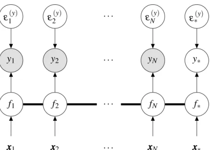
Fig. 3 illustrates a graphical model to represent the relations between the vari-ables previously defined for the standard GP model for noisy regression. The observations are shown as filled nodes and the latent (unobserved) variables as white nodes. Since the inputs xxxiare not random, they are shown as deterministic variables. The observation noise

y

y

···

y

y

ε

ε

···

ε

ε

f

f

···

f

f

xxx

xxx

···

xxx

xxx

Figure 3 – Graphical model detailing the relations between the variables in a standard GP model. The observations are shown as filled nodes and the latent (unobserved) variables as white nodes. The thick bar that connects the latent variables fi

indicates that all the those variables are connected between themselves.

It is important to highlight some points in Fig. 3: (i) an observation yi is

conditionally independent of the other nodes given its associated latent function variable

fi and observation noiseε( y)

i , which implies p(yyy|fff) =∏iN=1p(yi|fi); (ii) the thick bar that

connects the latent variables fiindicates that all the those variables are connected between

themselves, which is expected from the definition of the covariance matrix KKKf (see Eq.

(2.4)); (iii) the prediction f_∗ is part of the same GP prior that models the N training samples, which justifies the joint distribution in Eq. (2.10).

Alternatively (and more extensively), we could obtain the predictive expressions in Eq. (2.9) following a more formal Bayesian approach by first calculating the posterior distribution of fff given observed data via Bayes’ rule, which is tractable1 _{in this case:}

p(fff_|yyy,XXX)

| {z }

posterior =

likelihood

z }| { p(yyy_|fff)

prior

z }| { p(fff_|XXX)

p(yyy_|XXX)

| {z }

marginal likelihood

p(fff_|yyy,XXX)∝N _(yyy|fff,σ2

yIII)N (fff|000,KKKf) p(fff_|yyy,XXX) =N _{(fff|KKKf(KKKf+σ}2

yIII)−1yyy,(KKK−f1+σ−

2

y III)−1), (2.11)

where the marginal likelihood acts as a normalization term and the final expression is obtained by working the product of the likelihood and the prior and then “completing the

1

square”2.

Now that we have both the likelihood p(yyy_|fff) and the posterior p(fff_|yyy,XXX), inference for a new output f_∗ given a new input xxx_∗ is obtained with the tractable integral below, which marginalizes (integrates out) the latent variable fff:

p(f_∗|yyy,XXX,xxx_∗) =

Z

fff

p(f_∗|fff,XXX,xxx_∗)p(fff_|yyy,XXX), where p(f_∗|fff,XXX,xxx_∗) =N _{(f∗|kkk∗fKKK}−1

f ttt,K∗−kkk∗fKKK−

1

f kkkf∗) (see Eq. (2.2)), p(f_∗|yyy,XXX,xxx_∗) =N _{(f∗|µ∗,σ}2

∗),

µ_∗=kkk_∗f(KKKf+σy2III)−1yyy,

σ_∗2=K_∗−kkk_∗f(KKKf+σy2III)−1kkkf∗,

which is equal to Eq. (2.9). We emphasize that many of the previous expressions are only tractable because of the GP prior and Gaussian likelihood. For instance, if the likelihood is not Gaussian, which implies non-Gaussian observations, inference would not be analytical anymore. In such case, as in Chapter 4 of this thesis, where we consider non-Gaussian heavy-tailed likelihoods, approximation methods are required.

Fig. 4 shows a priori and a posteriori samples, i.e., before and after the observation of some outputs (represented by the small black dots). Note that larger values of w2 (smaller lengthscales) are related to wigglier functions. Note also that when noisy outputs are considered (σ2

y >0) the uncertainty around the observations is not close to

zero anymore.

Remark The sampled curves shown in Fig. 4 illustrate a typical issue faced by nonlinear machine learning method: the finite (and possibly noisy) training set is responsible for the existence of multiple models that are able to explain the observations. Thus, one should be careful when choosing a single instance within a class of models and do so by following a clearly defined metric.

2.4 Bayesian Model Selection

Differently from parametric regression methods, GP models do not have param-eters that concentrate the knowledge obtained from the training set. The only unknown

2

(a) Prior withw2=0.5 andσ2

y =0. (b) Posterior withw2=0.5 andσy2=0.

(c) Posterior withw2=0.5 andσ2

y =0.01. (d) Posterior withw2=5andσy2=0.01.

Figure 4 – Samples from the GP model before and after the observations. In all cases

σ2

f =1 was used.

model components are the kernel and noise hyperparameters. The noise variance σ2

y is

usually included in the vector of kernel hyperparameters θθθ, whose length becomesD+2, a quantity often much smaller than, for example, the number of weights in a multilayer neural network.

Figure 5 – Illustration of the Bayesian model selection procedure, where models too simple or too complex are avoided. The vertical axis indicates the evidence of a given model. Note that models with intermediate complexity present a balance between the value of the evidence and the number of possible supported datasets. Figure adapted from Rasmussen and Williams (2006).

marginalizing fff, is given by

logp(yyy_|XXX,θθθ) =logN _{(yyy|000,KKKf+σ}2 yIII),

=₋N

2log(2π)− 1 2log

KKKf+σy2III

| {z }

model capacity

−1₂yyy⊤ KKKf+σy2III −1

yyy

| {z }

data fitting

, (2.12)

which follows the marginal likelihood derived in Eq. (2.8), but now we explicitly denote the dependency on the vector of hyperparameters θθθ, which is used to compute the covariance matrixKKKf+σy2III3. Thedata fitting term highlighted in Eq. (2.12) is the only one containing

the observations yyy. The other highlighted term is related to the model capacity and is equivalent to a complexity penalty. Thus, model selection by evidence maximization automatically balances between those two components. This procedure is also known as type II maximum likelihood, since the optimization is in the hyperparameter space, instead of the parameter space (RASMUSSEN; WILLIAMS, 2006). Fig. 5 illustrates such Bayesian selection methodology, where the preferred model should be an intermediate one, neither too simple nor too complex, which is able to efficiently explain a given dataset without being too restrictive or too generic.

The optimization of such model selection problem is guided by the analytical

3

Algorithm 1: Standard GP modeling for regression. - Estimation step

Require: XXX _∈RN×D _{(inputs), yyy∈}RN _(outputs)

Initialize model hyperparameters θθθ =hσ2_f,w2₁,_···,w2_D,σ_y2i⊤; repeat

Compute the model evidence logp(yyy_|XXX,θθθ) via Eq. (2.12).

Compute the analytical gradients ∂logp_{∂ θ}(_θθyyy|XXX,θθθ) via the Eq. (2.13);

Updateθθθ with a gradient-based method (e.g. BFGS (FLETCHER, 2013)); until convergence or maximum number or iterations

Output the optimized hyperparameters θθθML;

- Test step

Require: xxx_∗∈RD _{(inputs), θ}θθML

Compute the predictive mean µ_∗ and variance σ_∗2 via the Eq. (2.9); Output y_∗∼N _µ∗,σ2

∗+σy2

;

gradients of the evidence with respect to each component of θθθ:

∂logp(yyy_|XXX,θθθ)

∂ θθθ =−

1

2Tr (KKKf+σ 2

yIII)−1

∂(KKKf+σy2III) ∂ θθθ

!

+1 2yyy

⊤_(KKK

f+σy2III)−1

∂(KKKf+σy2III)

∂ θθθ (KKKf+σ

2

yIII)−1yyy.

(2.13)

After the optimization, σ2

f is proportional to the overall variance of the output,

while σ2

y becomes closer to the observation noise variance. The optimized ARD

hyper-parameters w2₁, . . . ,w2_D are able to automatically turn off unnecessary dimensions of the input by taking values close to zero. Importantly, the model selection procedure does not involve any grid or random search, mechanisms usually needed for other kernel methods. Algorithm 1 summarizes the use of the standard GP modeling framework for regression.

2.5 From Feature Spaces to GPs

Despite the easiness of explaining the GP modeling approach from the function space view, as in Sections 2.2 and 2.3, it is useful to present the same expressions derived in a different manner.

Let φ :RD_→RV _{be a feature mapping function, from aD-dimensional space} to a V-dimensional space, and www_∈RV _{a vector of weights (or parameters). Using the} same notation for inputs and outputs of previous sections, wwwcan be used in the standard Bayesian linear (in the parameters) regression model below:

yi=www⊤φ(xxxi) +ε_i(y), ε_i(y)∼N (0,σy2). (2.14)

If we consider a zero mean Gaussian prior p(www) =N _(www|000,ΣΣΣ_w)over the weights, with covariance matrix ΣΣΣ_w∈RV×V_{, and define} ΦΦΦ₌φ(XXX)_∈RV×N _{as a matrix where each} column is given by φ(xxxi), after the application of the Bayes’ rule we get the posterior

p(www_|yyy,XXX) = p(yyy|www,XXX)p(www)

p(yyy_|XXX) =N www

1

σ2

y

AAA−1ΦΦΦyyy,AAA−1 !

, (2.15)

whereAAA_∈RV×V ₌ 1 σ2

y Φ

ΦΦΦΦΦ⊤+ΣΣΣ−_w1.

Given a new input xxx_∗, prediction is performed by averaging the weights, i.e., integrating out www:

p(f_∗|xxx_∗,XXX,yyy) =

Z

www

p(f_∗|xxx_∗,www)p(www_|yyy,XXX) =N _f∗

1

σ2

y

φ(xxx_∗)⊤AAA−1ΦΦΦyyy,φ(xxx_∗)⊤AAA−1φ(xxx_∗)

!

. (2.16)

We can rewrite the predictive distribution using the definition of the matrix AAA

and the two matrix identities below:

AAA−1ΦΦΦ= 1

σ2

y

ΦΦΦΦΦΦ⊤+ΣΣΣ−_w1

!−1

Φ

ΦΦ=σ_y2ΣΣΣ_wΦΦΦΦΦΦ⊤ΣΣΣ_wΦΦΦ+σ_y2III−1,

A

AA−1= 1

σ2

y

ΦΦΦΦΦΦ⊤₊ΣΣΣ−_w1

!₋1

=ΣΣΣ_w−ΣΣΣ_wΦΦΦΦΦΦ⊤ΣΣΣ_wΦΦΦ₊σ_y2III −1

Φ ΦΦ⊤ΣΣΣ_w,

where the second expression is the so-called matrix inversion lemma. The first identity is directly used in the mean of Eq. (2.16), while the lemma is applied in the variance. The new prediction then becomes

p(f_∗|xxx_∗,XXX,yyy) =N _f∗

φ(xxx∗)⊤ΣΣΣwΦΦΦ(ΦΦΦ⊤ΣΣΣwΦΦΦ+σy2III)−1yyy,

φ(xxx_∗)⊤ΣΣΣ_wφ(xxx_∗)₋φ(xxx_∗)⊤ΣΣΣ_wΦΦΦ(ΦΦΦ⊤ΣΣΣ_wΦΦΦ+σ_y2III)−1ΦΦΦ⊤ΣΣΣ_wφ(xxx_∗).

We can define some quantities by applying the kernel trick and the definition of a kernel function (SMOLA; SCH ¨OLKOPF, 2002):

Φ Φ

Φ⊤ΣΣΣ_wΦΦΦ=ΦΦΦTΣΣΣ1_w/2ΣΣΣ_w1/2ΦΦΦ=ΩΩΩ⊤ΩΩΩ=k(XXX,XXX) =KKKf, φ(xxx_∗)⊤ΣΣΣ_wΦΦΦ=k(xxx_∗,XXX) =kkk_∗f,

ΦΦΦ⊤ΣΣΣ_wφ(xxx_∗) =k(XXX,xxx_∗) =kkkf∗,

φ(xxx_∗)⊤ΣΣΣ_wφ(xxx_∗) =k(xxx_∗,xxx_∗) =K_∗,

where we have denoted ΩΩΩ as a modified feature map obtained from the input and replaced the inner product of such mapping by the kernel matrix KKKf. It is important to emphasize

that the actual mapping is never performed explicitly, but only by using the kernel function. Finally, by replacing the new kernel expressions back in Eq. (2.17), we get the standard predictive expression for GP models:

p(f_∗|xxx_∗,XXX,yyy) =N _{(kkk∗f(KKKf+σ}2

yIII)−1yyy,K∗−kkk∗f(KKKf+σy2III)−1kkkf∗). (2.18) Now we can see that GP regression is related to Bayesian regression with basis functions, i.e., linear combination of possibly nonlinear mappings, where a Gaussian prior is given to the weights, which are analytically integrated out. We emphasize that such integration is equivalent to consider infinitely many weights pondered by their priors. Furthermore, it is well known from the kernel learning literature, that many kernel functions, such as the previously mentioned exponentiated quadratic (Eq. (2.4)) is related to an infinite-dimensional feature space ΩΩΩ (SMOLA; SCH ¨OLKOPF, 2002).

Perhaps even more interestingly, in the chapter entitled Priors for Infinite Net-works in his thesis (NEAL, 1994), Neal demonstrated that within the Bayesian formalism, neural networks with one hidden layer containing infinitely many hidden neurons converge to a GP when Gaussian priors are assigned to the neurons’ weights. Furthermore, he also stated that such model should be able to avoid the risk of overfitting. Later, Williams (1998) derived the covariance function related to such infinity limit.

2002). Connections with kernel extensions to classical adaptive filters, such as the kernel recursive least-squares (KRLS) (ENGEL et al., 2004) and kernel least mean squares (KLMS) (LIU et al., 2008) algorithms have also been studied by Vaerenbergh et al. (2012)

and Vaerenbergh et al. (2016), respectively.

2.6 Sparse GP Models

A problem usually associated with GP models is its O_(N3_{) computation}

com-plexity and O_(N2_{) memory requirement}4_{, related to the predictive expression in Eq. (2.9)}

and the evidence in Eq. (2.12). The latter is more critical, since along with the gradients in Eq. (2.13), it needs to be computed every iteration of the optimization procedure. When the number of samples N is larger than a few thousands, the matrix inverse and determinant operations can be slow or even prohibitive.

Several authors have proposed different solutions to deal with this problem. Most of such methods were covered by Qui˜nonero-Candela and Rasmussen (2005), where a unifying view for sparse GP modeling is presented, highlighting the implicit approximations considered by each approach.

Later, a sparse approximate GP framework was proposed by Titsias (2009a), following a variational Bayes approach (SCHWARZ, 1988; JORDAN et al., 1999; GIBBS; MACKAY, 2000). Such approach has been proven to be flexible and effective by other authors, for instance in the recent works by Matthews et al.(2016) and Baueret al.(2016). Since Titsias’ variational sparse framework, sometimes called the variational free energy approximation, is applied within several models addressed by this thesis, we will describe it in more detail here. We follow the original presentation by Titsias (2009a) and the one presented by Damianou (2015). The reader is referred to Qui˜nonero-Candela and Rasmussen (2005) and Rasmussen and Williams (2006) to learn more about other sparse GP approaches.

2.6.1 The Variational Sparse GP Framework