Fiscal Episodes, Technological Progress and Market Power

(1)

António Afonso & João Tovar Jalles

Fiscal Episodes, Technological Progress and

Market Power

WP09/2015/DE/UECE

_________________________________________________________

De pa rtme nt o f Ec o no mic s

WORKING PAPERS

(2)

Fiscal Episodes, Technological Progress and

Market Power

*

July 2015

António Afonso

$

and João Tovar Jalles



Abstract

We assess the impact of fiscal adjustments (and technology) on the evolution of markups in a panel of 14 OECD countries. We allow for smooth changes in the technological parameters by generating measures of TFP compatible with markups and assess the interaction between the two variables. Our results with narrative action-based data show counter-cyclicality since negative fiscal shocks increase markups. Moreover, in times of economic contraction the degree of counter-cyclicality of negative (positive) government spending (tax) shocks is larger than during economic expansions. In addition, markups have a pro-cyclical behaviour after a productivity shock. However, when identifying fiscal consolidations using changes of the cyclically adjusted primary balance, one obtains expansionary effects and a pro-cyclical behaviour in terms of markups and aggregate demand shocks.

JEL: D4, E3, E6, H6

Keywords: imperfect competition, TFP, fiscal consolidation, local projection, business cycle, impulse response functions, GMM

*_{We thank comments from participants at the 4}th_{UECE Conference on Economic and Financial Adjustments in Europe}

(Lisbon). The opinions expressed herein are those of the authors. The usual disclaimer applies and any remaining errors

are the authors’ sole responsibility.

$_ISEG/ULisbon_–_{University of Lisbon, Department of Economics; UECE}_–_{Research Unit on Complexity and}

Economics, R. Miguel Lupi 20, 1249-078 Lisbon, Portugal, email: [email protected]. UECE is supported by the Portuguese Foundation for Science and Technology through national funds via the Strategic Project: UID/ECO/00436/2013. email: [email protected].

_{Center for Globalization and Governance, Nova School of Business and Economics, 1099-032 Lisboa, Portugal. email:}

(3)

2

1. INTRODUCTION

The interaction between fiscal policy effectiveness and imperfect competition has received some attention in economic theory (Hall, 2009; Christiano et al., 2011; Woodford, 2011, and the survey by Costa and Dixon, 2011). In particular, the cyclical behaviour of markups following government spending shocks has been closely analyzed. The New Keynesian Synthesis has developed models that produce undesired endogenous markups due to nominal rigidity, enhancing the effectiveness of demand-side policy, including fiscal policy. Moreover, macroeconomic models with time-varying desired markups are even more attractive as they work similarly to productivity shocks in the presence of active fiscal policy (Ravn et al., 2006).

The theoretical literature on endogenous markups is dominated by the view that markups behave counter-cyclically following a demand shock. When a positive shock originates in the demand side, such as a government spending shock, the marginal cost function is only indirectly affected and the main effect depends on how the individual demand function responds (see e.g. Gali, 1994a, b; Clarida et al. 1999; Goodfriend and King, 1997; Hairault and Portier, 1993; Ravn et al., 2006). However, with a positive supply shock (or TFP shock), we expect marginal costs to decrease for a given output. Therefore, assuming that the indirect effect on prices via demand is small, markups tend to increase implying a pro-cyclical average markup.

Several papers that try to measure markups for different industries over a period find evidence of a mildly counter-cyclical behaviour (Hall, 1988; Martins and Scarpetta, 2002; Rotemberg and Woodford, 1991, 1999). The combination of demand and supply shocks is a possible explanation for the existing evidence on countercyclicality. Recently Monacelli and Perotti (2008), Nekarda and Ramey (2010), Juessen and Linnemann (2012) and Afonso and Costa (2013) analyzed the effects of

fiscal policy on markups’ behaviour both in country-specific VARs and in a panel VAR.

(4)

3

adjusted primary balance (CAPB) as a quantitative approach to identifying fiscal episodes (including fiscal expansions), as well as assessing how the role of other macroeconomic and structural factors impact the markup’s cyclicality behaviour.

Our results show that negative fiscal shocks stemming from fiscal retrenchments (either a decrease in expenditure or an increase in taxes) in the fiscal stance lead to a rise in the markup up until 4 years after the start of the fiscal episode. Moreover, in times of economic contraction the degree of counter-cyclicality of negative (positive) government spending (tax) shocks is much larger than in times of economic expansion.

In addition, markups have a pro-cyclical behaviour after a productivity shock (markups increase up to 4 years alongside the positive response of GDP), an outcome consistent with most existing endogenous markups hypotheses.

However, since when using CAPB-based methods one gets evidence of expansionary fiscal effects, there is a pro-cyclical behaviour in terms of markups and aggregate demand shocks in that case. This result raises some already existing concerns about the use of CAPB-based approaches and the need to expand the use of narrative methods.

The remainder of the paper is organized as follows. Section 2 briefly outlines the framework of the markup. Section 3 presents the data and econometric methodology. Section 4 discusses the empirical results and section 5 concludes.

2. THE MARKUP

The markup is the price wedge,

(1)

where represents the price of the good produced by firm i and stands for its marginal cost,

in t.

Since marginal costs are not observable, one can estimate them using the relationship where is the nominal wage rate (with homogeneous labour input) and is the marginal product of labor. The production function is represented by Yit = F(Lit,), with

technology given by



1



. t. t

t t t t t

(5)

4

At being TFP, 0 < t < 1, and t > 0, and Afonso and Costa (2013) assume that the production

function has namely a positive decreasing MPLit.

The data for the markup are from Afonso and Costa (2013).1 Therefore, we also used a set of 14

OECD countries for which there were data on average markups for a long period (1970-2007) and the macroeconomic variables were taken from the European Commission AMECO database (see

Afonso and Costa’s, 2013 notation and definitions below):

- represents real GDP per capita, i.e., per head between 15 and 64 years old, measured in 2000 PPPs;

- stands for real capital stock per capita, measured in 2000 PPPs;

- is total hours worked, i.e., the product of average hours per employee and total employment, per capita;

- represents the adjusted wage share in total income, (which was adjusted using the ratio between the concepts of employment and number of employees that exist in the national accounts for domestic industries), and the long-run labour share is st* = 1 - t.

3. DATA AND ECONOMETRIC METHODOLOGY

3.1.1 Computing fiscal episodes

The literature addressing the identification of fiscal episodes is vast and has, for a long time, relied on changes in the cyclically adjusted primary balance (CAPB). Nevertheless, some caveats surrounding this approach have also been highlighted. In particular, the CAPB approach could bias empirical estimates towards finding evidence of non-Keynesian effects (see Afonso and Jalles, 2014). Many non-policy factors, such as price fluctuations, influence the CAPB and can lead to erroneous conclusions regarding the presence of fiscal policy changes.2 In addition, even when the CAPB accurately measures fiscal actions these include discretionary responses to economic developments, such as fiscal tightening to restrain rapid domestic demand growth.

Therefore, with the above mentioned considerations in mind, an alternative “narrative approach” is considered, which relies on the identification of fiscal episodes on the basis of concrete

1_{This markup data set is available at:}

https://aquila4.iseg.ulisboa.pt/aquila/homepage/f619/research/datasets/afonso-and-costa:-market-power-and-fiscal-policy-in-oecd-countries.

2_{For example, a stock price boom raises the CAPB by increasing capital gains tax revenue, and also tends to coincide}

(6)

5

policy decisions. The episodes are identified by looking at IMF and OECD historical reports and by checking what countries intended to do at the time of publication.3 This policy-action based approach makes use of descriptive historical facts that usually describe what happened to the budget deficit in a particular period but they do not go into the details of policy makers' intentions, discussions and congressional records. Proponents of this approach argue that the estimated size of the fiscal measures during the episodes identified have the advantage of not being affected by the

cycle (since their construction is “bottom-up”), can minimize identification problems,4_{and are}

unlikely to imply risks of reverse causation (Guajardo and others, 2014). That said, the narrative approach could also have some drawbacks: it largely relies on judgment calls, and it may not eliminate entirely endogeneity problems (i.e., fiscal policy reacting to the output performance and not the other way around). The analysis that follows relies on both the narrative and CAPB-based approaches. On the former, the analysis uses the publicly available dataset compiled by Devries and others (2011) based on the policy-action based method for advanced economies between 1978 and 2009. On the latter, we begin in 1970 and the analysis relies on Giavazzi and Pagano’s (1996)

approach under which a fiscal episode consists of a change in the CAPB at least 5, 4, 3 percentage points of GDP in respectively 4, 3 or 2 years, or 3 percentage points in one year.

Other approaches used for robustness purposes include: i) Alesina and Ardagna (1998), who adopted a fiscal episode definition that allows that some stabilization periods may have only one year, that is, they consider the change in the primary cyclically adjusted budget balance that is at least 2 percentage points of GDP in one year or at least 1.5 percentage points on average in the last

two years; and ii) Afonso’s (2010) under which a fiscal episode occurs when either the change in the CAPB (as a percentage of potential GDP) is at least one and a half times the standard deviation (from the reference country panel) in one year, or when the change in the CAPB is at least one standard deviation on average in the last two years.

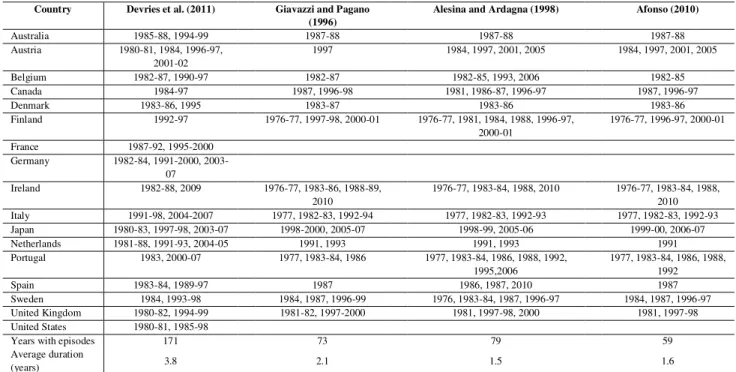
Table 1 reports the fiscal episodes identified according to the above-mentioned four alternative methods (table retrieved from Afonso and Jalles, 2014). The number of fiscal contractions ranges from 29, in the approach proposed by Afonso (2010), to 43, using the approach from Alesina and

Ardagna (1998). In the Devries et al.’s (2011) narrative approach the magnitude of the fiscal

3_{Note, however, that this approach differs from the one used in Romer and Romer (2010), who identify exogenous tax}

policy changes by analyzing US congressional documents.

(7)

6

consolidation episode ranges between 0.1 percent and about 5 percent of GDP, with an average of about 1 percent of GDP. Moreover, it reports a much higher number of years where fiscal contractions take place (171 years against an average of 70 for the CAPB approaches). For fiscal consolidations, the average duration of the reported fiscal episodes is, on average, 1.7 years for the CAPB approaches and around 3.8 years for the narrative approach. Moreover, the three CAPB-based methods essentially coincide in about 50% of total number of years with those of the narrative approach.

[Table 1]

3.2 Estimating Impulse Response Functions

To estimate the impact of fiscal adjustments (and technology) on the evolution of markups over the short and medium-run, we follow the method proposed by Jorda (2005) which consists of estimating impulse response functions (IRFs) directly from local projections. For each period k the

following equation is estimated on annual data:

(3) with k=1,…,5 (in years) and where Y represents our markup variable; is a vector that includes

fiscal consolidations (a dummy taking the value 1 at the beginning of the episode and zero otherwise) and technology (proxied by the logarithm of TFP) in country i at time t; are country

fixed effects; is a time trend; and measures the impact of for each future period k.

Since fixed effects are included in the regression the dynamic impact should be interpreted as compared to a baseline country-specific trend. In the main results, the lag length (l) is set at 2, even

if the results are extremely robust to different numbers of lags included in the specification (see robustness checks and sensitivity presented in the next section). Equation (3) is estimated using the panel-corrected standard error (PCSE) estimator (Beck and Katz, 1995).

(8)

7

estimation of and in small samples (Nickell, 1981), the length of the time dimension mitigates this concern.5_{Robustness checks for endogeneity confirm the validity of the results.}

An alternative way of estimating the dynamic impact of fiscal consolidation episodes (or technology) is to estimate an ARDL equation of changes in the markup and consolidation episodes (or technology) and to compute the IRFs from the estimated coefficients (Romer and Romer, 1989; and Cerra and Saxena, 2008). However, the IRFs derived using this approach tends to be sensitive to the choice of the number of lags, making the IRFs potentially unstable. In addition, the significance of long-lasting effects with ARDL models can be simply driven by the use of one-type-of-shock models (Cai and Den Haan, 2009). This is particularly true when the dependent variable is highly persistent, as in our analysis. In contrast, the approach used here does not suffer from these problems because the coefficients associated with the lags of the change in the dependent variable enter only as control variables and are not used to derive the IRFs, and since the structure of the equation does not impose permanent effects. Finally, confidence bands associated with the estimated IRFs are easily computed using the standard deviations of the estimated coefficients and Montecarlo simulations are not required.

4. EMPIRICAL ANALYSIS

4.1 Baseline Results

Prior to presenting and discussing our main empirical results, one concern when working with time-series data is the possibility of spurious correlation between the variables of interest (Granger and Newbold, 1974). This situation arises when series are not stationary. We implement three different types of panel unit root tests: two first generation tests, namely the Im et al. (2003) test (IPS); the Maddala and Wu (1999) test (MW) and one second generation test – the Pesaran (2007) CIPS test. The latter is associated with the fact that previous tests do not account for cross-sectional dependence of the contemporaneous error terms and failure to consider it may cause substantial size distortions in panel unit root tests (Pesaran, 2007). Tables A1 and A2 in the Appendix show the results for the levels of TFP and the markup and reveal that the null unit root hypothesis can be rejected in the latter case but not in the former (first differences of TFP will be used).

(9)

8

Moreover we employ a recent panel data stationarity test which under the null hypothesis of panel stationarity takes multiple structural breaks into account (Carrion-i-Silvestre et al., 2005-CBL hereafter)6_{. The authors developed this instrument for panels including individual fixed effects} and/or an individual-specific time trend. It also has the capability to consider multiple structural breaks positioned at different unknown dates in addition to varying numbers of breaks for each individual. This test is of special interest for our purposes because structural breaks do not have to be restricted just for the purposes of preventing level shifts. The test of the null hypothesis of a stationary panel follows the estimation of the number of structural breaks and their position is based on the procedure in Bai and Perron (1998), which computes the overall minimization of the sum of the squared residuals.7_{Results of the test (which synchronously is a panel and individual data} stationarity test with multiple structural breaks8_{) are presented in the Appendix Table A3. We find} that when we allow for cross-section dependence and when we use the bootstrap critical values, the null of stationarity cannot be rejected for the markup at usual levels by either the homogeneous or heterogeneous long-run version of the test. The same does not apply for TFP. All in all, evidence confirms previous findings, notably for the lack of stationarity of TFP, even after multiple structural breaks and cross-section dependence are allowed for.

The short and medium-term impacts of the fiscal consolidations and TFP on markups are shown in Figure 1 for the baseline regression. Each graph shows the estimated impulse response function and the associated one standard error bands (dotted lines), where the horizontal axis measures years.

In general, a negative fiscal shock associated with a fiscal retrenchment in the fiscal stance leads to a rise in the markup up until 4 years after the start of the episode. Thus, for the panel as a whole markups present a countercyclical behaviour following a decrease in expenditure (or an increase in taxes) associated with a consolidation episode, since a negative shock to government expenditure decreases GDP (see Figure 1a-a and Figure 1b-d). Hence, results favour endogenous

6_{We thank Josep Carrion-i-Silvestre for providing his GAUSS code.}

7_{We estimate the number of structural breaks associated with each individual using the modified Schwarz information}

criteria. CBL (2005) suggested that in the empirical process, the specified maximum number of structural breaks is 5. We compute the finite sample critical values using Monte Carlo simulations with 20,000 replications; in order words, we approximate the empirical distribution of the panel data statistic by means of bootstrap techniques to get rid of the cross-section independence assumption.

(10)

9

countercyclical markups for demand shocks (see Hall, 2009): a fiscal adjustment, or similarly negative demand shock, implies a shift to the left in the demand curve and a leftward movement along the marginal cost curve when output decreases, with a higher increase in prices that the one observed in marginal costs.

On the other hand, markups present a pro-cyclical behaviour after a productivity shock (markups increase up to 4 years alongside the positive response of GDP) and this outcome is consistent with most existing endogenous markups hypotheses, either of the undesired or of the desired kinds (see Figure 1a-b and Figure 1b-e).

Figure 1.a Baseline (PCSE): Response of Markups to Fiscal Consolidations, TFP and GDP shocks

a) Impulse of Consolidation

-0.01 -0.008 -0.006 -0.004 -0.002 0 0.002 0.004 0.006 0.008 0.01

0 1 2 3 4 5

estimate lower limit upper limit

b) Impulse of TFP

-0.1 -0.05 0 0.05 0.1 0.15 0.2

0 1 2 3 4 5

c) Impulse of GDP

-1.2 -1 -0.8 -0.6 -0.4 -0.2 0

0 1 2 3 4 5

Figure 1.b Baseline (PCSE): Response of GDP to Fiscal Consolidations, TFP and Markup shocks

d) Impulse of Consolidation

-0.012 -0.01 -0.008 -0.006 -0.004 -0.002 0 0.002 0.004 0.006

0 1 2 3 4 5

e) Impulse of TFP

-0.05 0 0.05 0.1 0.15 0.2 0.25 0.3

0 1 2 3 4 5

f) Impulse of Markup

0 0.02 0.04 0.06 0.08 0.1 0.12 0.14 0.16 0.18

0 1 2 3 4 5

Note: Dotted lines equal one standard error confidence bands. See main text for more details. Horizontal axis indicates years after the shock. PCSE - panel-corrected standard error.

4.2 Robustness

(11)

10

broadly unchanged. Moreover, as shown by Tuelings and Zubanov (2010), a possible bias from estimating Equation (3) using country-fixed effects is that the error term of the equation may have a non-zero expected value, due to the interaction of fixed effects and country-specific fiscal developments. This would lead to a bias of the estimates that is a function of k. to address this issue

and check the robustness of our findings, Equation (3) was re-estimated by excluding country fixed effects from the analysis. The results (not shown but available upon request) suggest that this bias is negligible (the difference in the point estimate is small and not statistically significant). As an additional sensitivity check, Equation (3) was re-estimated for different lags (l) of changes in the

markup. The results for zero lags and three lags (not shown but available upon request) confirm that previous findings are not sensitive to the choice of the number of lags. Moreover, using alternative markups and the corresponding TFP measures provided similar results.

Furthermore, estimates of the impact of fiscal consolidations (or technology) on markups could be biased because of endogeneity, as unobserved factors influencing the dynamics of public finances may also affect the probability of the occurrence of a consolidation episode. In particular, a significant deterioriation in economic activity, which would affect unemployment, may determine an increase in the public debt ratio via automatic stabilizers, and therefore increase the probability of consolidation. To address this issue, Equation (3) was augmented to control for the output gap (computed by means of the HP filter with a smoothing parameter of 6.25 applied to real GDP). The results of this exercise (not shown but available upon request) confirm the robustness of the previous findings.

Figure 2. Robustness (GMM): Response of Markups to Fiscal Consolidations and TFP shocks a) Impulse of Consolidation

-0.015 -0.01 -0.005 0 0.005 0.01 0.015

0 1 2 3 4 5

b) Impulse of TFP

-0.1 -0.05 0 0.05 0.1 0.15

0 1 2 3 4 5

(12)

11

Moreover, an alternative way to deal with endogeneity concerns is to re-estimate Equation (3) by means of a GMM estimator such as the Arellano and Bover (1995). This estimator is particularly relevant when series are very persistent and the lagged levels may be weak instruments in the first differences. In this case, lagged values of the first differences can be used as valid instruments in the equation in levels and efficiency is increased by regressing Equation (3) with the use of a system GMM estimator.9_{Figure 2 shows the results and confirms the findings discussed} above. Finally, using alternative measures of markups (see Afonso and Costa, 2013) – not shown –

does not qualitatively alter our main conclusions.

4.3 Alternative definitions of fiscal consolidations

So far we have based our results on the use of the Devries et al. (2011) narrative approach dataset. We also use now the method of identifying fiscal episodes using changes in the CAPB. Taking the three alternative approaches detailed in Section 3 and re-estimating Equation (3) for Giavazzi and Pagano’s (1996), Alesina and Ardagna’s (1998) and Afonso’s (2010) alternative

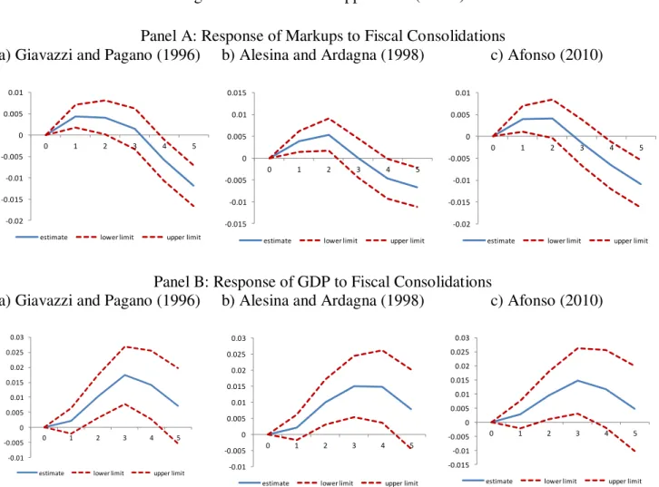
approaches to identify fiscal episodes, gives the IRFs displayed in Figure 3. In general, we still find that fiscal consolidations lead to an increase in markups

However, and as illustrated elsewhere (see e.g. Afonso and Jalles, 2014) the use of CAPB-based methods to identify fiscal consolidation episodes can result in expansionary effects on output. This is exactly what we observe in Panel B where a fiscal consolidation episode delivers an expansionary fiscal consolidation result. Therefore, when using the CAPB as a measure of the fiscal episodes, we have, in this case, a pro-cyclical behaviour in terms of markups and aggregate demand shocks. This section’s result highlights the concerns about the use of CAPB-based approaches and the need to expand the use of narrative methods. For the remainder of the paper we will focus on the narrative method.

9_{The list of instruments includes the first and second lags of all the right-hand-side variables. The null of Hansen J-test}

(13)

12

Figure 3. CAPB-based Approaches (PCSE) Panel A: Response of Markups to Fiscal Consolidations

a) Giavazzi and Pagano (1996) b) Alesina and Ardagna (1998) c) Afonso (2010)

-0.02 -0.015 -0.01 -0.005 0 0.005 0.01

0 1 2 3 4 5

-0.015 -0.01 -0.005 0 0.005 0.01 0.015

0 1 2 3 4 5

-0.02 -0.015 -0.01 -0.005 0 0.005 0.01

0 1 2 3 4 5

Panel B: Response of GDP to Fiscal Consolidations

a) Giavazzi and Pagano (1996) b) Alesina and Ardagna (1998) c) Afonso (2010)

-0.01 -0.005 0 0.005 0.01 0.015 0.02 0.025 0.03

0 1 2 3 4 5

estimate lower limit upper limit -0.01

-0.005 0 0.005 0.01 0.015 0.02 0.025 0.03

0 1 2 3 4 5

-0.015 -0.01 -0.005 0 0.005 0.01 0.015 0.02 0.025 0.03

0 1 2 3 4 5

Note: Dotted lines equal one standard error confidence bands. See main text for more details. Horizontal axis indicates years after the shock.

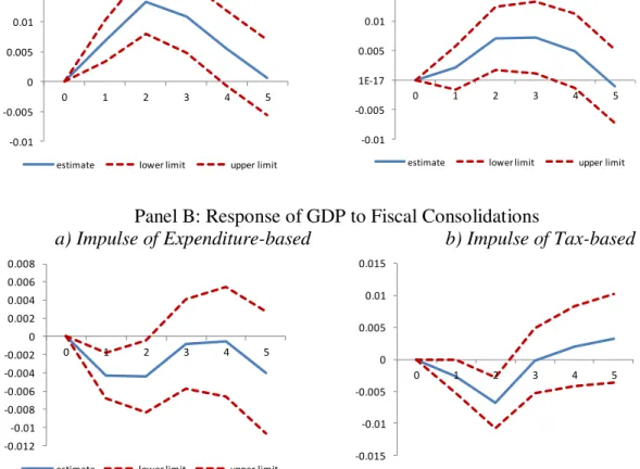
4.4 Composition of Fiscal Consolidation

Does the composition of fiscal consolidation (expenditure versus taxes-driven) matter for

(14)

13

Figure 4. Expenditure vs. Tax-Based Adjustments (PCSE) Panel A: Response of Markups to Fiscal Consolidations

a) Impulse ofExpenditure-based

-0.01 -0.005 0 0.005 0.01 0.015 0.02

0 1 2 3 4 5

b) Impulse ofTax-based

-0.01 -0.005 1E-17 0.005 0.01 0.015 0.02

0 1 2 3 4 5

Panel B: Response of GDP to Fiscal Consolidations

a) Impulse ofExpenditure-based

-0.012 -0.01 -0.008 -0.006 -0.004 -0.002 0 0.002 0.004 0.006 0.008

0 1 2 3 4 5

b) Impulse ofTax-based

-0.015 -0.01 -0.005 0 0.005 0.01 0.015

0 1 2 3 4 5

This result however has to be treated with caution given that most of past fiscal adjustments have involved both spending cuts and tax increases. In order to address this issue, following Guajardo et al. (2014), Equation (3) is separately estimated for: i) episodes where taxes-based adjustments have been larger than spending adjustments; 2) episodes where spending adjustments have been larger than tax based adjustments. These correspond to the “alternative definition” of tax

(15)

14

upon request) confirm that spending-based consolidations tend to have larger (positive) impact on markups.10

4.5 The role of the Business Cycle Phase: Good times vs. Bad times

In order to explore whether cyclicality varies depending on the phase of the business cycle, the following alternative regression will be estimated:

(4)

with

where z is an indicator of the state of the economy (using the output gap) normalized to have zero

mean and unit variance.11 The remainder of the variables and coefficients are defined as in Equation (3).

Still with the narrative-action based dataset, in times of economic contraction the degree of counter-cyclicality of negative (positive) government spending (tax) shocks is much larger than in times of economic expansion (Figure 5). In fact, during booms, the response of markups to a fiscal adjustment is pro-cyclical. This remains true even when one splits between expenditure and tax-based consolidations. One can admit that the size of the fiscal multiplier would tend to be lower on the spending side. For instance, a reduction in public wages can have a demonstration effect to private wages allowing for higher firm profits, more private investment, and the overall effect on GPD would be more mitigated than via the tax based fiscal consolidation.

10_{It must be recognized that also this approach is imperfect. Indeed, to properly differentiate between spending versus}

tax-based consolidations one should consider episodes characterized by only spending or taxes-based adjustments. This

however would dramatically reduce the number of “pure” spending and taxes-based consolidations in our sample.

11 _{This approach is equivalent to the smooth transition autoregressive (STAR) model developed by Granger and}

(16)

15

Figure 5. The role of the Business Cycle Phase: a shock to fiscal consolidations (PCSE)

Bad Times Good Times

Panel A: Impulse ofOverall Consolidations

Response of Markups

-0.03 -0.02 -0.01 0 0.01 0.02 0.03 0.04 0.05 0.06

0 1 2 3 4 5

-0.03 -0.02 -0.01 0 0.01 0.02 0.03 0.04 0.05 0.06

0 1 2 3 4 5

Response of GDP

-0.06 -0.05 -0.04 -0.03 -0.02 -0.01 0

1 2 3 4 5 6

0 0.01 0.02 0.03 0.04 0.05 0.06

1 2 3 4 5 6

Panel B: Impulse ofExpenditure based Consolidations

Response of Markups

-0.04 -0.03 -0.02 -0.01 0 0.01 0.02 0.03 0.04 0.05

0 1 2 3 4 5

-0.04 -0.03 -0.02 -0.01 0 0.01 0.02 0.03 0.04 0.05

0 1 2 3 4 5

Response of GDP

-0.06 -0.05 -0.04 -0.03 -0.02 -0.01 0

1 2 3 4 5 6

0 0.01 0.02 0.03 0.04 0.05 0.06

1 2 3 4 5 6

(17)

16

Panel C: Impulse ofTax based Consolidations

Response of Markups

-0.03 -0.02 -0.01 0 0.01 0.02 0.03 0.04

0 1 2 3 4 5

estimate lower limit upper limit _-0.03

-0.02 -0.01 0 0.01 0.02 0.03 0.04

0 1 2 3 4 5

Response of GDP

-0.06 -0.05 -0.04 -0.03 -0.02 -0.01 -2E-17 0.01

1 2 3 4 5 6

0 0.01 0.02 0.03 0.04 0.05 0.06

1 2 3 4 5 6

(18)

17

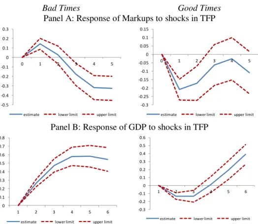
Figure 6. The role of the Business Cycle Phase: a shock to TFP (PCSE)

Bad Times Good Times

Panel A: Response of Markups to shocks in TFP

-0.5 -0.4 -0.3 -0.2 -0.1 0 0.1 0.2 0.3

0 1 2 3 4 5

-0.3 -0.25 -0.2 -0.15 -0.1 -0.05 0 0.05 0.1 0.15

0 1 2 3 4 5

Panel B: Response of GDP to shocks in TFP

0 0.1 0.2 0.3 0.4 0.5 0.6 0.7 0.8

1 2 3 4 5 6

-0.3 -0.2 -0.1 0 0.1 0.2 0.3 0.4 0.5 0.6

1 2 3 4 5 6

Note: Dotted lines equal one standard error confidence bands. See main text for more details.

4.6 The role of structural factors

We now assess whether the effect of fiscal consolidation and productivity shocks on the behaviour of markups depends on countries’ structural, macroeconomic and policy variables:

indebtedness (debt-to-GDP ratio), country size (population), trade openness (exports plus imports over GDP), level of economic development (real GDP per capita) and institutional settings (political constraints).

To test whether the factors mentioned above affect the response of markups to negative fiscal shocks and positive TFP shocks, Equation (3) is re-estimated using these variables’ 2nd_{quartile as}

the threshold value to split the whole sample into two sub-samples that will be compared against the baseline.

(19)

18

Moreover, the positive impact of a TFP shock on the markups’ behaviour is larger in bigger countries.

Figure 7.1 The role of Structural Factors (PCSE): Response of Markups to Fiscal Consolidations and TFP shocks

a) Impulse of Fiscal Consolidation b) Impulse of TFP

-0.008 -0.006 -0.004 -0.002 0 0.002 0.004 0.006 0.008 0.01

0 1 2 3 4 5

average low debt high debt

-0.3 -0.25 -0.2 -0.15 -0.1 -0.05 0 0.05 0.1 0.15

0 1 2 3 4 5

average low debt high debt

-0.01 0 0.01 0.02 0.03 0.04 0.05 0.06

0 1 2 3 4 5

average low size high size

-0.5 -0.4 -0.3 -0.2 -0.1 0 0.1 0.2

0 1 2 3 4 5

average low size high size

Note: Lines represent the impulse responses of markups to fiscal consolidation and TFP shocks (panels a) and b) respectively). Blue line denotes the baseline (full) sample result; the dotted green and dotted red lines denote the corresponding groups as identified in the legends when they are statistically significantly different from zero (otherwise they are equal to the baseline). The threshold point for each structural factor considered corresponds to the 2nd_{quartile (above/below). See main text for more details. Horizontal axis indicates years after the shock.}

In Figure 7.2 results show that countries more open to international trade and with larger

(20)

19

Figure 7.2 The role of Policy and Macro Factors (PCSE): Response of Markups to Fiscal Consolidations and TFP shocks

-0.01 -0.005 0 0.005 0.01 0.015 0.02

0 1 2 3 4 5

average low openness high openness

-0.25 -0.2 -0.15 -0.1 -0.05 0 0.05 0.1 0.15

0 1 2 3 4 5

average low openness high openness

-0.015 -0.01 -0.005 0 0.005 0.01 0.015

0 1 2 3 4 5

average low development high development

-0.3 -0.25 -0.2 -0.15 -0.1 -0.05 0 0.05 0.1 0.15 0.2 0.25

0 1 2 3 4 5

average low development high development

Note: vide footnote figure 8.1

The literature on fiscal policy has generally pointed out that a key factor in explaining differences across countries in the conduct of fiscal policy is the quality of political institutions. The results suggest that countries characterized by a lower quality of institutions generally tend to be characterized by worse fiscal outcomes in terms of debt levels, government size, spending volatility and cyclicality of fiscal deficits (Persson, 2001; Persson and Tabellini, 2001; Alesina et al., 2008). In Figure 7.3 we get the result that in countries with higher political constraints the degree of

markups’ countercyclicality following a negative fiscal shock is larger while the degree of

(21)

20

Figure 7.3 The role of Institutions (PCSE): Response of Markups to Fiscal Consolidations and TFP shocks

-0.01 -0.005 0 0.005 0.01 0.015 0.02

0 1 2 3 4 5

average low political constraints high political constraints

-0.2 -0.15 -0.1 -0.05 0 0.05 0.1 0.15

0 1 2 3 4 5

average low political constraints high political constraints

Note: vide footnote figure 8.1

5. CONCLUSION

We assess the impact of fiscal adjustments and TFP shocks on the evolution of average markups in a panel of 14 OECD countries for a long period between 1970 and 2007. We use alternative approaches to identify fiscal consolidations (cyclically adjusted primary balance and narrative action-based) and allow for smooth changes in the technological parameters by generating measures of TFP compatible with markups to assess the interaction between the two variables. Econometrically, we resort to impulse response analysis estimated directly from local projections.

Using the narrative-action based approach we find that a negative fiscal shock associated with a fiscal retrenchment (either a decrease in expenditure or an increase in taxes) in the fiscal stance leads to a rise in the markup up until 4 years after the start of the episode: a countercyclical result. On the other hand, markups present a pro-cyclical behaviour after a productivity shock (markups increase up to 4 years alongside the positive response of GDP) and this outcome is consistent with most existing endogenous markups hypotheses. Our main results are robust to several sensitivity checks such as the inclusion of time fixed effects, the exclusion of country fixed effects, alternative lag specifications, different definitions of markups, augmented set of controls and alternative estimators.

(22)

21

Additional empirical exercises reveal that spending-based consolidation programs have a more counter-cyclical effect on the behaviour of markups over the short and medium term than tax-based ones. Moreover, in times of economic contraction the degree of counter-cyclicality of negative (positive) government spending (tax) shocks is much larger than in times of economic expansion. Results also seem to support some symmetry in the results, in the sense that the short-term impact of fiscal expansions on markups is negative, therefore corroborating the counter-cyclicality. Finally, we uncovered that the role of structural, macroeconomic and policy variables does matter, particularly in the short-term.

REFERENCES

1. Afonso, A., 2010, “Expansionary Fiscal Consolidations in Europe: New Evidence,” Applied Economics Letters, 17(2), 105–9.

2. Afonso, A., and J. T. Jalles, 2014, “Assessing Fiscal Episodes,” Economic Modeling, 37, 255–70. 3. Afonso, A., L. Costa, 2013, “Market Power and Fiscal Policy in OECD countries”, Applied Economics, 45 (32), 4545-4555.

4. Alesina, A., and S. Ardagna, 1998, “Tales of Fiscal Adjustments,” Economic Policy, 489–545. 5. Alesina, A., Campante, F., and Tabellini, G. (2008), “Why is fiscal policy often procyclical?”,

Journal of the European Economic Association, 6(5), 1006-1036.

6. Arellano, M. and O. Bover 1995. “Another look at the instrumental variable estimation of error -components models.” Journal of Econometrics, 68, 29-52

7. Bai, J. and P. Perron, 1998, “Estimating and testing linear models with multiple structural changes”,

Econometrica 66, 47-78.

8. Beck, N. L., and J. N. Katz. 1995. “What to do (and not to do) with time-series cross-section data”.

American Political Science Review, 89, 634–647.

9. Cai, X., and W. J. Den Haan. 2009. “Predicting Recoveries and the Importance of Using Enough

Information”, CEPR Discussion Paper No. 7508.

10. Carrión-i-Silvestre, J.L., T. Del Barrio, and E. López-Bazo, 2005, “Breaking the panels. An application to the GDP per capita”, Econometrics Journal 8, 159-175.

11. Cerra, V., and S. Saxena, 2008, “Growth Dynamics: The Myth of Economic Recovery,” American

Economic Review, 98(1), 439-57.

12. Christiano, Lawrence, Martin Eichenbaum, and Sergio Rebelo. 2011. “When is the Government Spending Multiplier Large?” Journal of Political Economy, 119(1), 78-121.

13. Clarida, R., Galí, J. and Gertler, M. (1999). “The Science of Monetary Policy: A New Keynesian Perspective”. Journal of Economic Literature 37, 1661-1707.

(23)

22

15. Devries, P., J. Guajardo, D. Leigh, and A. Pescatori, 2011, “A New Action-Based Dataset of Fiscal

Consolidation,” IMF Working Paper No. 11/128 (Washington: International Monetary Fund).

16. Galí, J., 1994a. “Monopolistic Competition, Business Cycles, and the Composition of Aggregate Demand”. Journal of Economic Theory 63(1), 73-96.

17. Galí, J., 1994b. “Monopolistic Competition, Endogenous Markups, and Growth”. European

Economic Review 38(3-4), 748-756.

18. Giavazzi, F., and M. Pagano, M., 1996, “Non-Keynesian Effects of Fiscal Policy Changes:

International Evidence and the Swedish Experience,” Swedish Economic Policy Review, Vol. 3, No. 1, pp. 67–103.

19. Goodfriend, M. and King, R., 1997. “The New Neo-Classical Synthesis and the Role of Monetary

Policy”. NBER Macroeconomics Annual 231-283.

20. Guajardo, J., D. Leigh, and A. Pescatori, 2014, “Expansionary Austerity: New International Evidence,” Journal of the European Economic Association, 12(4), 949-968.

21. Hairault, J.-O. and Portier, F., 1993. “Money, New-Keynesian Macroeconomics and the Business

Cycle”. European Economic Review 37(8), 1533-1568.

22. Hall, R., 1988. “The Relationship between Price and Marginal Cost in U.S. Industry”. Journal of Political Economy 96(2), 921-947.

23. Hall, R., 2009. “By How Much Does GDP Rise If the Government Buys More Output?” NBER

Working Papers 15496.

24. Hall, Robert E. 2009. “By How Much Does GDP Rise if the Government Buys More Output?”

Brooking Papers on Economic Activity, 183-249.

25. M, K. S., Pesaran, M. H. and Shin, Y., 2003, “Testing for unit roots in heterogeneous panels”,

Journal of Econometrics 115, 53-74.

26. Jordà, Ò., 2005, “Estimation and Inference of Impulse Responses by Local Projections,” American Economic Review, 95(1), 161–82.

27. Jordà, Ò., and A. M. Taylor, 2013, “The Time for Austerity: Estimating the Average Treatment Effect of Fiscal Policy,” Federal Reserve Bank of San Francisco Working Paper 2013/25 (San Francisco:

U.S. Federal Reserve Bank).

28. Juessen, F., and L. Linnemann, 2010, “Estimating Panel VARs from Macroeconomic Data: Some

Monte Carlo Evidence and an Application to OECD Public Spending Shocks”, Mimeo

29. _{Maddala, G. S., & Wu, S. (1999), “A comparative study of unit root tests with panel data and a new} simple test”, Oxford Bulletin of Economics and Statistics, 61(Special Issue), 631-652.

30. Martins, J.O. and Scarpetta, S., 2002. “Estimation of the Cyclical Behaviour of Mark-ups: A

technical note”. OECD Economic Studies 34(1), 173-188.

31. Monacelli, T. and Perotti, R., 2008. _{“Fiscal Policy, Wealth Effects, and Markups”. NBER Working} Paper 14584.

32. Morris, R., and L. Schuknecht, 2007, “Structural Balances and Revenue Windfalls: The Role of Asset Prices Revisited,” ECB Working Paper No. 737 (Frankfurt: European Central Bank).

33. _{Nekarda, C.J., and V. Ramey, 2010, “The cyclical}behaviour of the price-_{cost markup”, manuscript,} University of California, San Diego

(24)

23

35. Persson, T. (2001), “Do political institutions shape economic policy?”, NBER Working Paper 8214.

36. Persson, T. and Tabellini, G. (2001), “Political institutions and policy outcomes: what are the stylized facts?”, CEPR Discussion Papers 2872.

37. Pesaran, M. H., 2007, “A simple panel unit root test in the presence of cross-section dependence”,

Journal of Applied Econometrics, 22(2), 265-312.

38. Ravn, M., Schmitt-Grohé, S., and Uribe, M., 2006. “Deep habits”. Review of Economic Studies, 73(1), 195–218

39. Romer, C., and D. Romer, 1989, “Does Monetary Policy Matter? A New Test in the Spirit of

Friedman and Schwartz,” NBER Macroeconomics Annual, 4, 121–70.

40. Romer, C., and D. Romer, 2010, “The Macroeconomic Effects of Tax Changes: Estimates Based on

a New Measure of Fiscal Shocks,” American Economic Review, 100 (3), 763–801.

41. Rotemberg, J. and Woodford, M., 1991. “Markups and the Business Cycle”. NBER Macroeconomics

Annual 6, 63-128.

42. Rotemberg, J. and Woodford, M., 1999. “The Cyclical Behaviour of Prices and Costs”. In: Taylor, J.

and Woodford, M., (Eds.) Handbook of Macroeconomics, Elsevier, Amsterdam, 1051-1135.

43. Teulings, C. N., and N. Zubanov, 2010, “Economic Recovery a Myth? Robust Estimation of Impulse

Responses,” CEPR Discussion Papers No. 7800 (London: Center for Economic Policy Research).

44. Woodford, Michael. 2011. “Simple Analytics of the Government Expenditure Multiplier.” American

(25)

24

Table 1: Fiscal contraction episodes based on the change in the primary cyclically adjusted budget balance and on the narrative approach

Country Devries et al. (2011) Giavazzi and Pagano (1996)

Alesina and Ardagna (1998) Afonso (2010)

Australia 1985-88, 1994-99 1987-88 1987-88 1987-88

Austria 1980-81, 1984, 1996-97,

2001-02

1997 1984, 1997, 2001, 2005 1984, 1997, 2001, 2005

Belgium 1982-87, 1990-97 1982-87 1982-85, 1993, 2006 1982-85

Canada 1984-97 1987, 1996-98 1981, 1986-87, 1996-97 1987, 1996-97

Denmark 1983-86, 1995 1983-87 1983-86 1983-86

Finland 1992-97 1976-77, 1997-98, 2000-01 1976-77, 1981, 1984, 1988, 1996-97,

2000-01

1976-77, 1996-97, 2000-01

France 1987-92, 1995-2000

Germany 1982-84, 1991-2000,

2003-07

Ireland 1982-88, 2009 1976-77, 1983-86, 1988-89,

2010

1976-77, 1983-84, 1988, 2010 1976-77, 1983-84, 1988,

2010

Italy 1991-98, 2004-2007 1977, 1982-83, 1992-94 1977, 1982-83, 1992-93 1977, 1982-83, 1992-93

Japan 1980-83, 1997-98, 2003-07 1998-2000, 2005-07 1998-99, 2005-06 1999-00, 2006-07

Netherlands 1981-88, 1991-93, 2004-05 1991, 1993 1991, 1993 1991

Portugal 1983, 2000-07 1977, 1983-84, 1986 1977, 1983-84, 1986, 1988, 1992,

1995,2006

1977, 1983-84, 1986, 1988, 1992

Spain 1983-84, 1989-97 1987 1986, 1987, 2010 1987

Sweden 1984, 1993-98 1984, 1987, 1996-99 1976, 1983-84, 1987, 1996-97 1984, 1987, 1996-97

United Kingdom 1980-82, 1994-99 1981-82, 1997-2000 1981, 1997-98, 2000 1981, 1997-98

United States 1980-81, 1985-98

Years with episodes 171 73 79 59

Average duration

(years) 3.8 2.1 1.5 1.6

(26)

25

Appendix

Table A1: First Generation Panel Unit Root Tests

Im, Pesaran and Shin (2003) Panel Unit Root Test (IPS) (a)

Full markup TFP

in levels

lags [t-bar] lags [t-bar]

1.14 -11.258** 1.43 0.918

Maddala and Wu (1999) Panel Unit Root Test (MW) (b)

Full markup TFP

lags p (p) p (p)

in levels

0 120.806 0.00 3.243 1.00 1 207.140 0.00 17.261 0.94 2 142.865 0.00 19.82 0.87 3 129.492 0.00 21.21 0.81

Notes: (a) We report the average of the country-specific “ideal” lag-augmentation (via AIC). We report the t-bar statistic, constructed as





bar N iti

t (1/ ) (tiare country ADF t-statistics). Under the null of all country series containing a nonstationary process this statistic has a

non-standard distribution: the critical values are -1.73 for 5%, -1.69 for 10% significance level – distribution is approximately t. We indicate the cases where the null is rejected with **. (b) We report the MW statistic constructed as __₂_log( ₎

i i p

p_ (piare country ADF statistic p-values) for

different lag-augmentations. Under the null of all country series containing a nonstationary process this statistic is distributed 2(2 )

N

 . We further report the p-values for each of the MW tests.

Table A2: Second Generation Panel Unit Root Tests

Pesaran (2007) Panel Unit Root Test (CIPS)

Full markup TFP

lags p (p) p (p) in levels

0 -6.416 0.00 6.945 1.00 1 -8.080 0.00 -0.115 0.45 2 -6.503 0.00 -1.758 0.04 3 -4.895 0.00 -2.818 0.00 Notes: Null hypothesis of non-stationarity. We further report the p-values for each of the CIPS tests.

Table A3: CBL (2005) Panel Unit Root Tests allowing for multiple breaks

Variable markup

KPSS test Test statistics Bootstrap critical values

90% 95% 97.5% 99%

Homogeneity -3.689 2.093 3.007 3.951 5.129 Heterogeneity -2.681 2.010 2.696 3.586 4.444

Variable TFP

KPSS test Test statistics Bootstrap critical values

90% 95% 97.5% 99%

Homogeneity 3.582** 2.506 3.386 4.515 5.397 Heterogeneity 2.947* 2.252 2.952 3.509 4.425