Binary programming for the simulation of crop rotation and animal
transit in an integrated crop-livestock system
1Programação binária para simulação de rotações de culturas e trânsito animal em
sistema integrado lavoura-pecuária
Deumara Galdino de Oliveira2*, Angel Ramon Sanchez Delgado3, Sergio Drumond Ventura3, Marcelo Dib Cruz3
and Paulo Cesar Parga Rodrigues3
ABSTRACT - The aim of this study was to develop and implement a linear-programming model (LP) that provides as its result a schedule with the best selection of crops in each plot per period, and with the greatest weight gain for each animal. The linear-programming model was developed from empirical work carried out by Alvarenga and Gontijo Neto (2008) in an area of 24 hectares ofEmbrapa Milho e Sorgo, in Sete Lagoas, Minas Gerais (MG). For the computational implementation of the model, it was necessary to have data on agricultural suitability and animal weight gain for each period and for each plot. In order to test the developed mathematical model, values were randomly generated for agricultural suitability and for animal weight gain using the MATLAB solver. It was then possible to carry out the computational implementation of the linear-programming model in MATLAB. Two numerical trials were conducted, the first considering four periods, four plots and the transit of two animals, and the second with ten periods, four plots and the transit of three animals. The results show that the linear-programming model is consistent with the empirical work done by Alvarenga and Gontijo Neto (2008). The linear-programming model satisfies all the imposed constraints, maximises the weight gain of each animal, and provides the best selection of crops.
Key words: Planning. Sustainability. Binary programming in crop and livestock farming.
RESUMO -O objetivo é desenvolver e implementar um modelo de programação linear (PL) que forneça como resultado um cronograma com a melhor seleção de cultivos em cada gleba por período e com o maior ganho de peso de cada animal. O modelo de programação linear foi desenvolvido a partir do trabalho empírico realizado por Alvarenga e Gontijo Neto (2008) implantado naEmbrapa Milho e Sorgo (Sete Lagoas, MG) em uma área de 24 hectares. Para a implementação computacional do modelo são necessários os dados sobre aptidão agrícola e ganho de peso do animal em cada período e em cada gleba. A fim de testar o modelo matemático desenvolvido, gerou-se valores para aptidão agrícola e para o peso ganho pelo animal de forma aleatória utilizando o solver do MATLAB. Com isso, pode-se realizar a implementação computacional do modelo de programação linear no MATLAB. Foram realizados dois ensaios numéricos, o primeiro considerando quatro períodos, quatro glebas e trânsito de dois animais e o segundo com dez períodos, quatro glebas e trânsito de três animais. Os resultados mostram que o modelo de programação linear é compatível com o trabalho empírico realizado por Alvarenga e Gontijo Neto (2008). O modelo de programação linear satisfaz todas as restrições impostas, maximiza o ganho de peso de cada animal e fornece a melhor seleção de cultivos.
Palavras-chave: Planejamento. Sustentabilidade. Programação binária na agropecuária.
DOI: 10.5935/1806-6690.20190015 *Author for correspondence
Received for publication in 07/04/2014; approved in 03/04/2018
1Parte da Tese de Doutorado apresentada pelo primeiro autor ao Programa de Pós-graduação em Ciência, Tecnologia e Inovação em Agropecuária,
UFRRJ/Seropédica
2Programa de Pós-Graduação em Ciência, Tecnologia e Inovação em Agropecuária/PPGCTIA, Universidade Federal Rural do Rio de Janeiro/UFRRJ,
BR 465, Km 7, Seropédica-RJ, Brasil, 23.851-000, [email protected]
3Departamento de Matemática, Universidade Federal Rural do Rio de Janeiro/UFRRJ, BR 465, Km 7, Seropédica- RJ, Brasil, 23.851-000, asanchez@
INTRODUCTION
Sustainability in crop and livestock farming is negatively affected by traditional soil management and by the degradation of pasture. To minimise the fall in productivity, it is necessary to increase investment in the sector to recover degraded pastures and eroded soils, making the system unsustainable. Hence the need to invest
in soil conservation (BALBINOet al., 2011; MACEDO,
2009; SILVA et al., 2012; TELLES; GUIMARAES;
DECHEN, 2011).
The search for alternatives that lead to agricultural practices carried out safely in order to guarantee present and future productivity is increasing, and such practices must be combined with reduced environmental impact
(PATO et al., 2008). Adequate management promotes
an increase in the recovery of greenhouse gases (GHG), which are so damaging to the environment (CARVALHO
et al., 2010). In addition, the conservation of plant cover
effectively contributes to the sustainability of these activities (BORGESet al., 2014).
Crop-Livestock Integration (CLI) is a production system offering such benefits as diversified food production; an improvement in the physical, chemical and biological conditions of the soil; the replenishment of organic matter; a reduction in the costs of agricultural activity through optimisation of the use of inputs; and the control of weeds, pests and diseases (SALTONet al.,
2015; SILVEIRA; STONE, 2003).
It is in the context of the search for a sustainable increase in productivity that crop-livestock integration gains strength, because it provides the best use of the soil for agricultural and livestock activities developed in the same area, ensuring their economic viability (BARBIERI
et al., 2013; COBUCCIet al., 2007; SOUZAet al., 2012).
Such use can be obtained through the management of these activities by intercropping, in succession or even by rotation.
The adoption of crop-livestock integration is complex, and it is necessary to plan the actions to be implemented when adopting this type of management so that the producer is successful. Martha Júnior, Alves and Contini (2011) state that the various demands of adopting CLI must be met; otherwise, the success of this type of management would be compromised. For Balbinot Junior (2009), the sustainability of CLI is a consequence of the relationship established between biological, economic and social factors.
The aim of this study is the development of a binary-programming model (NEMHAUSER; WOLSEY, 1999), which simulates the rotation of agricultural crops and the transit of animals under a CLI system. The Integer
Programming Problem is a type of linear-programming problem in which the variables must assume the values 0 or 1, known as a binary program. This type of program is widely used when searching for solutions, where value 1 means that the characteristic is present and value 0 means it is absent.
As in other areas, binary integer programming can be used in farming to achieve the efficient use of resources. In an area divided into lots, 0-1 programming means that 1 indicates a particular crop is grown in the lot and 0 indicates that the crop does not grow in the lot. The result is a timeline for developing activities. This mathematical model was developed based on the empirical work carried out by Alvarenga and Gontijo Neto (2008) in an area of 24
hectares of Embrapa Milho e Sorgo (Sete Lagoas, MG).
The result of the mathematical model is consistent with this empirical work.
MATERIAL AND METHODS
Crop Rotation
In order to carry out the mathematical modelling and computational implantation of the rotational and strategic planning of crops, the crop-livestock integration system
implemented in an area of 24 hectares byEmbrapa Milho
e Sorgo (Sete Lagoas, MG) (ALVARENGA, GONTIJO
NETO, 2008) was considered as the scenario. With this technology, planning must be carried out, because the plots sometimes have to be used with crops and at other times as pasture.
Accordingly, areas of Soybean (S), Pasture (P), Maize+Grass (M+G) and Sorghum+Grass (S+C) are considered within a predetermined planning horizon (number of periods), and an ‘optimal’ schedule of crop rotation (intercropped or not with pasture) is developed for each period and each plot. It is assumed that each crop is grown in one, and only one plot of the area under consideration. Here the optimal is the maximum ‘adaptation’ or weight that any one crop has when grown in a determined plot during a particular period. In general, a schedule of crops with maximum weight is sought.
It can be assumed that by means of a physical and chemical analysis of the soil in each plot, a physiological criterion can be established, based on the adaptation and growth of each crop in a given period; from this criterion, values between zero and one be are allocated to each crop, indicating the percentage advantage that the crop has in relation to the remainder when it is grown in that plot and during that period.
horizon (periods), an optimal rotational crop schedule is determined through mathematical modelling and computational implementation.
Following is the mathematical model that represents the determination of an optimal rotational crop schedule from randomly generated data. It is begun by indicating with i- Periods (i = 1,...,m), j- Tracts
or Lots (j = 1,...,n; n ≥ 4), and k- Crop, where k = 0 (Pasture), k = 1 (Soybean), k = 2 (Maize+Grass), k = 3 (Sorghum+Grass).
In addition, the following variables are defined:
xijk = 1 If during periodicropk is grown in plotj
= 0 If otherwise.
Let pijk be the weight allocated by the growth of cropk in plotjduring periodi.
Constraints:
1. During any given periodi, each cropk, should be
grown (or not) in one, and only one plotj.
k = 0, 1, 2, 3; i = 1,..., m (1)
j = 1,...,n; i = 1, ...,m Se n = 4 (2)
j = 1,…, n; i = 1,…,m Se n > 4 (3)
2. If during periodi, cropk is grown in plotj, then
cropk cannot be grown in plot j during period i + 1.
xijk + xi+1jk ≤ 1 i = 1,...,m – 1; j = 1,..., n; k = 0, 1, 2, 3 (4)
3. If during period i pasture (k = 0) is grown in
plotj, then during periodi + 1, soybean (k = 1) should be
grown in plotj.
xij0 – xi+1j1 ≤ 0 i = 1,...,m – 1; j = 1,...,n (5)
4. If during periodi, soybean (k = 1) is grown in
plot j, then during the following period i + 1, in plot j,
Maize+Grass (k = 2) or Sorghum+Grass (k = 3) should be grown.
xij1 – xi+1j2 – xi+1j3 ≤ 0 i = 1,...,m – 1; j = 1,...,n (6)
5. If during period i, Maize+Grass (k = 2) is
developed in plotj, then during the following periodi+ 1,
in plotj, pasture (k = 0) or Sorghum+Grass (k = 3) should
be grown.
xij2 – xi+1j0 – xi+1j3 ≤ 0 i = 1,...,m – 1; j = 1,...,n (7)
6. If during period i, Sorghum+Grass (k = 3) is
grown in plotj, then during the following periodi + 1, in
plot j, pasture (k = 0) or Maize+Grass (k = 2) should be
grown.
xij3 – xi+1j0 – xi+1j2 ≤ 0 i = 1,...,m – 1; j = 1,..., n (8)
Maximising the Objective Function
(9)
Animal Traffic
Rotating between crops and pasture as a strategy for agricultural production, in addition to improving soil properties and reducing the incidence of insect pests, diseases and weeds, it offers the benefit of better stability of forage production to feed the herd throughout the year. Below, the operational control of animal transit will focus on live weight and on the number of periods estimated until the animal is slaughtered. Following is the mathematical model representing the determination of the optimal animal transit from randomly generated data.
Consider the indices r = 1,…,p (Animals) and the parameters PVri Live weight of animal r during period i
(kg), PVAri - Live weight gain for the slaughter of animalr
during periodi (kg) and gijr - Gain in live weight of animal r in plotj during periodi (kg).
For each i=1,…,m, consider Si = {r:PVri < PVAri} and = {r:PVri << PVAri}.
Both sets indicate those animals with insufficient live weight for slaughter or extremely low live weight for slaughter respectively.
Variables:
yijr = 1 If during periodi animalr is found in plotj
= 0 If otherwise.
Constraints:
1. If during period i, plot j is between crops of
Maize+Grass and animali has insufficient live weight for
slaughter, then this animal should remain in plotj during
periodi.
(xij2 – yijr) ≤ 0 i = 1,...,m; j = 1,...,n; r ϵ Si (10) 2. If during period i, plot j is between crops of
Sorghum+Grass and animalr has insufficient live weight
for slaughter, then this animal should remain in plot j
during periodi.
(xij3 – yijr) ≤ 0 i = 1,...,m; j = 1,...,n; r ϵ Si (11) 3. If during periodi, plot j is under Pasture and
animalr has extremely low live weight for slaughter, then
this animal should remain in plotj during periodi.
4. If during periodi, soybean (k = 1) is grown in
plotj, then animalr cannot be in plotj.
i = 1,...,m; j = 1,...,n (13)
Maximising the Objective Function
(14)
Binary-Programming Model for the Problem of Agricultural-Crop Rotation and Animal Traffic under a CLI System.
This model was constructed from the two models shown above by summing the respective objective functions and including the constraints of both models, thereby ensuring the rotation of crops and the issues related to animal transit, while observing the constraints.
Maximising the Objective Function
(15)
In order for the binary integer-programming model above to be used, there should also be information about agricultural suitability (pijk), which indicates the percentage advantage that one crop has over the other crops, and the live weight gained per animal (gijr). These values for agricultural suitability (pijk) and live weight gain (gijr) are determined for each period and for each plot.
With the aim of testing the mathematical model, values for agricultural suitability (pijk) and for live weight gain (gijr) were generated randomly with the MATLAB 7.4 solver, considering sets of rules (or a set of constraints) that guarantee that the soil and production be sustained. MATLAB is a solver, whose language is based on matrices, which allows various mathematical calculations to be performed, function graphs to be constructed and linear problems to be solved. Two numerical trials were
carried out, the first considering four periods, four plots and the transit of two animals, and the second with ten periods, four plots and the transit of three animals. Both trials were implemented in MATLAB using the integer-programming tutorial.
The procedure for generating random values is crucial to ensure that the above model can be used with real data. In addition, a comparison was made with the empirical work carried out by Alvarenga and Gontijo Neto (2008) in an area of 24 hectares ofEmbrapa Milho e Sorgo (Sete Lagoas, MG). The result was consistent with
the empirical model, i.e. the binary integer-programming model is valid.
RESULTS AND DISCUSSION
Table 1 shows the results obtained for four periods, four plots, two bulls and four crops (intercropped or not with pasture). It can be seen that constraint 1, relative to crop rotation, is satisfied, and indicates that for each period, each crop is grown in one, and only one plot. In addition, no crop is planted during any two consecutive periods, i.e. the constraints relating to equation (2) are satisfied, so crop rotation is ensured together with the cycling of nutrients.
Note that, as required by the constraints (3) for crop rotation in each plot, if in a given period pasture is grown, then during the following period soybean will be grown, which helps in not degrading the pasture. This results in a reduction in costs, since the costs for renovating or recovering degraded pastures is quite high.
Similarly for each plot, if in a given period soybean is grown, then in the following period Maize+Grass should be grown (see plot 1, plot 2 and plot 3). On the other hand, if Maize+Grass is grown in any period, during the
Table 1 - Optimal rotational crop schedule k=0 (Pasture), k=1 (Soybean), k=2 (Maize+Grass), k=3 (Sorghum+Grass) for four periods
and four plots, and the optimal transit schedule for two bulls (b1 and b2)
Period 1
Plot 1 Plot 2 Plot 3 Plot 4
Pasture Sorghum+Grass Soybean Maize+Grass
b1-b2 b1-b2 *-* b1-b2
Period 2 Soybean Pasture Maize+Grass Sorghum+Grass
*-* b1-b2 b1-b2 b1-b2
Period 3 Maize+Grass Soybean Sorghum+Grass Pasture
*-b2 *-* *-b2 *-b2
Period 4 Sorghum+Grass Maize+Grass Pasture Soybean
Table 2 - Indicators of the animals that have a live weight below
that for slaughter, with a value of one if the animal belongs to Si and zero if otherwise (m=4 and p=2)
following period Sorghum+Grass is grown (see plot 1, plot 3 and plot 4). Note the sequence Pasture, Soybean, Maize+Grass in plots 1 and 2.
It should be noted that the symbol * indicates that the animal reached the necessary weight for slaughter. In relation to the ‘weights’, and as mentioned above, it is possible to establish a physiological criterion based on the adaptation and development of each crop in a given area and a particular period, from which values between zero and one can be allocated to each crop, indicating the percentage advantage of that crop in relation to the other crops when it is grown in that plot and during that period. Table 2 shows which animals have a live weight below that for slaughter; a value of one (1) indicates that the live weight of the animal is below that for slaughter, and a value of zero (0) indicates that the animal has reached the weight for slaughter.
It can be seen that the weights of the animals are below that for slaughter during both the first and second periods. During the third period, the first bull (b1) reaches the weight for slaughter; however the second bull (b2) should be fed during the third and fourth periods in the first, third and fourth plots, and the first, second and third plots respectively.
In relation to the optimal schedule for animal transit, it can be seen that during the first period it is recommended that both animals (b1 and b2) be fed in each plot; except in plot 3, where soybean should be grown, and where animals are not allowed to remain, as per the constraints (4) of the binary integer-programming model for animal transit.
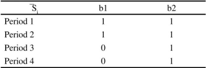
Table 3 shows the animals that have a live weight well below that for slaughter; a value of one indicates that the live weight of the animal is below that for slaughter and a value of zero (0) indicates that the animal has reached the required weight.
It can be seen that the weight of both animals is far below that for slaughter. In addition, during the second period,
Table 3 - Indicators of the animals that have a live weight well below that for slaughter, with a value of one if the animal belongs to Si and zero if otherwise (m=4 and p=2)
Si b1 b2
Period 1 1 1
Period 2 1 1
Period 3 0 1
Period 4 0 1
̅
Si b1 b2
Period 1 1 1
Period 2 1 1
Period 3 0 1
Period 4 0 1
both animals should be fed in plots 2, 3 and 4, since their live weight remains well below the weight for slaughter.
The results of the first numerical trial, which considered a total of four periods, four plots and two animals (b1, b2), show the validity of the model by satisfying all the imposed constraints and maximising the objective function, ensuring the weight gain of each animal and crop selection in each plot for each period being considered. Furthermore, because crop rotation is adopted, the inputs used for agricultural activity are rationalised and, as a result, production costs are reduced
(FRANCHINIet al., 2011).
Table 4 shows the schedule for ten periods, four plots and the transit of three animals. It can be seen that the constraints (1) regarding crop rotation are satisfied and indicate that for each period, each crop is grown in only one plot. In addition, no crop is grown for any two consecutive periods; i.e. the constraints relating to the equation for crop rotation (2) are satisfied. Note, that as required by the constraints (3) for crop rotation in each plot, if in a given period pasture is grown, then during the following period soybean will be grown.
Again, for each plot, if in a given period soybean is grown, then in the following period Maize+Grass (plot 2 and plot 3) or Sorghum+Grass (see plot 1, plot 2, plot 3 and plot 4) should be grown, as per the constraints (4) of the crop-rotation model.
On the other hand, if during any period Maize+Grass is grown, then during the following period Sorghum+Grass (see plot 1, plot 3 and plot 4) or Pasture (see plot 2, plot 3 and plot 4) should be grown, as per the constraints (5) of the crop-rotation model. Similarly, Sorghum+Grass should be followed by Maize+Grass (see plot 1, plot 3 and plot 4) or pasture (see plot 1 and plot 4), as per Constraint 6 of the crop-rotation model.
Constraint 4 of the model for animal transit is met; i.e. if in any one period, soybean (k=1) is grown in plotj,
then animalr cannot be in plotj. Thus, where soybeans are
Table 4 - Optimal rotational crop schedule k=0 (Pasture), k=1 (Soybean), k=2 (Maize+Grass), k=3 (Sorghum+Grass) for ten periods and four plots, and the optimal transit schedule for three bulls (b1, b2, b3)
There are multiple benefits from implementing the optimal rotational schedule for Pasture, Soybean, Maize+Grass and Sorghum+Grass, such as diversified food production; a reduction in the incidence of pests and diseases, very common in production systems based on monocropping; nutrient cycling; an improvement in the conditions of pasture, and a reduction in recovery costs by avoiding the processes of degradation.
Furthermore, it can be seen that by diversifying activities, the frequency of growing crops in each plot decreases. As a result, the negative effects of monocropping, such as a loss in productivity and degradation of the soil and natural resources, are reduced or even eliminated (LOSSet al., 2011), while at the same time, resources are
optimised, resulting in a reduction in farming costs, which contributes to the stability of the activity over the years, i.e. the production system is efficient.
Table 5 indicates which animals have a live weight below for that for slaughter; a value of one (1) indicates that the live weight of the animal is below that for slaughter and a value of zero (0) indicates that the animal has reached the weight for slaughter. In this table, it is
Period 1
Plot 1 Plot 2 Plot 3 Plot 4
Sorghum+Grass Maize+Grass Pasture Soybean
b1 - b2- b3 b1 - b2- b3 b1 - b2- b3 *-*-*
Period 2 Maize+Grass Pasture Soybean Sorghum+Grass
* - b2- b3 * - b2- b3 *-*-* * - b2- b3
Period 3 Sorghum+Grass Soybean Maize+Grass Pasture
*-2-3 *-*-* *-2-3 *-2-3
Period 4 Pasture Maize+Grass Sorghum+Grass Soybean
* - b2- b3 * - b2- b3 * - b2- b3 *-*-*
Period 5 Soybean Pasture Maize+Grass Sorghum+Grass
*-*-* *-*-* *-*-* *-*-*
Period 6 Sorghum+Grass Soybean Pasture Maize+Grass
*-*-* *-*-* *-*-* *-*-*
Period 7 Pasture Maize+Grass Soybean Sorghum+Grass
*-*-* *-*-* *-*-* *-*-*
Period 8 Soybean Pasture Sorghum+Grass Maize+Grass
*-*-* *-*-* *-*-* *-*-*
Period 9 Sorghum+Grass Soybean Maize+Grass Pasture
*-*-* *-*-* *-*-* *-*-*
Period 10 Maize+Grass Sorghum+Grass Pasture Soybean
*-*-* *-*-* *-*-* *-*-*
can be seen that during the first period, the three animals should be fed in the areas where pasture, Maize+Grass and Sorghum+Grass are cultivated. The animals reach the weight for slaughter during the second period.
Table 5 - Indicators of the animals that have a live weight below that for slaughter, with a value of one if the animal belongs to Si and zero if otherwise (m=10 and p=3)
Si b1 b2 b3
Period 1 1 1 1
Period 2 0 1 1
Period 3 0 1 1
Period 4 0 1 1
Period 5 0 0 0
Period 6 0 0 0
Period 7 0 0 0
Period 8 0 0 0
Period 9 0 0 0
Table 6 - Indicators of the animals that have a live weight well below that for slaughter, with a value of one if the animal belongs to Si and zero if otherwise (m=10 and p=3)
For the second period, b1 has enough weight for slaughter and therefore leaves sets Si and Ṡi, during this period, b2 and b3 remain below the weight for slaughter and should therefore be fed in the plots where Pasture, Maize+Grass and Sorghum+Grass are cultivated, as per the constraints (1, 2 and 3) of the binary integer-programming model for animal transit.
During the third and fourth periods, b2 and b3 are still below the weight for slaughter, and should be fed in the plots where soybean is not grown. Finally, from the fifth period, b1, b2 and b3 have sufficient live weight for slaughter.
Table 6 shows the animals that have a live weight well below that for slaughter; a value one (1) indicates that the live weight of the animal is below that for slaughter and a value of zero (0) indicates that the animal has reached the weight for slaughter. Animals b1 and b3 have a live weight well below that for slaughter, while the live weight of b2 is only just below the weight for slaughter; i.e. b2 does not belong to Ṡi. From the fifth period, none of the animals has a live weight well below that for slaughter.
̅
Si b1 b2 b3
Period 1 1 0 1
Period 2 0 0 1
Period 3 0 1 1
Period 4 0 1 1
Period 5 0 0 0
Period 6 0 0 0
Period 7 0 0 0
Period 8 0 0 0
Period 9 0 0 0
Period 10 0 0 0
The results obtained from the second numerical trial, which considered a total of ten periods, four plots and three animals (b1, b2, b3) also show the validity of the model by satisfying all imposed constraints and maximizing the objective function, ensuring for each period being considered the weight gain of each animal and the crop selection in each plot.
According to Gameiro, Caixeta Filho and Barros (2010), the great benefit from implementing linear-programming models in crop and livestock production
systems is due to their considering various pieces of information and offering the best solution as a result.
Therefore, the integer-programming model presented in this section not only provides the optimal solution in the face of imposed constraints, one that maximises the weight gain of each animal with the best selection of crops in each plot per period, but also allows the producer to check the variations in some attributes, further improving the results of the crop and livestock production system.
CONCLUSIONS
1. A binary program (BP) is presented that simulates crop rotation and animal transit, whose solution represents an optimal schedule for the crops considered in the crop-livestock integration technology developed in an area of 24 hectares at Embrapa Milho e Sorgo, as well as the simulation of animal transit;
2. To implement the binary integer-programming model, data are necessary on the number of lots, number of periods, values of the indicators of agricultural suitability (pijk) and live weight gain per animal (gijr). It should be pointed out that the model was implemented from random data for agricultural suitability (pijk) and for the live weight gained per animal (gijr) for each period in each plot, thereby generating the schedules presented in Tables 1 and 4. The result therefore depends on these parameters, i.e. different values for these weights (pijk) and for the weight gained per animal (gijr), would produce a different schedule than those presented; 3. Crop rotation is highly recommended for randomly
generated plots, and that result agrees with the experimental results obtained at Embrapa-Milho e Sorgo. Consequently, the mathematical model presented using binary programming is compatible with the empirical work by Alvarenga and Gontijo
Neto (2008) developed in an area of 24 hectares at
Embrapa Milho e Sorgo. From the results presented, it can be seen that it was possible to construct a mathematical model that meets the constraints of crop rotation, aiming at the efficient use of resources, and enabling the producer to verify the technical feasibility of adopting CLI on his property.
REFERENCES
BALBINO, L. C. et al. Evolução tecnológica e arranjos produtivos de sistemas de integração lavoura-pecuária-floresta no Brasil. Pesquisa Agropecuária Brasileira, v. 46, n. 10, p. i-xii, 2011.
BALBINOT JUNIOR, A. A.et al. Integração lavoura-pecuária:
intensificação de uso de áreas agrícolas.Ciência Rural, v. 39,
n. 6, p. 1925-1933, 2009.
BARBIERI, D. M.et al. Comportamento dos óxidos de ferro
da fração argila e do fósforo adsorvido, em diferentes sistemas de colheita de cana-de-açúcar. Revista Brasileira de Ciência do Solo, v. 37, n. 6, p. 1557-1568, 2013.
BORGES, W. L. B. et al. Absorção de nutrientes e alterações
químicas em Latossolos cultivados com plantas de cobertura em rotação com soja e milho.Revista Brasileira de Ciência do Solo, v. 38, n. 1, p. 252-261, 2014.
CARVALHO, J. L. N.et al. Potencial de sequestro de carbono
em diferentes biomas do Brasil.Revista Brasileira de Ciência do Solo, v. 34, p. 277-289, 2010.
COBUCCI, T.et al. Opções de Integração lavoura-pecuária e
alguns de seus aspectos econômicos.Informe Agropecuário,
v. 28, n. 240, p. 64-79, 2007.
FRANCHINI, J. C.et al. Importância da rotação de culturas para
a produção agrícola sustentável no Paraná. Londrina: Embrapa Soja, 2011, 47 p. (Documentos, 327).
GAMEIRO, A. H.; CAIXETA FILHO, J. V.; BARROS, C. S. Modelagem matemática para o planejamento, otimização e avaliação da produção agropecuária.In: SANTOS, M. V.et al.
Novos desafios da pesquisa em nutrição e produção animal.
Pirassununga: Editora 5D: Programa de Pós-Graduação em Nutrição e Produção Animal, 2010. 260 p.
LOSS, A.et al. Agregação, carbono e nitrogênio em agregados do
solo sob plantio direto com integração lavoura-pecuária.Pesquisa
Agropecuária Brasileira, v. 46, n. 10, p. 1269-1276, 2011. MACEDO, M. C. M. Integração lavoura e pecuária: o estado da arte e inovações tecnológicas.Revista Brasileira de Zootecnia, v. 38, p. 133-146, 2009. Suplemento especial.
MARTHA JÚNIOR, G. B.; ALVES, E.; CONTINI, E. Dimensão econômica de sistemas de integração lavoura-pecuária. Pesquisa Agropecuária Brasileira, v. 46, n. 10, p. 1117-1126, 2011.
MATLAB. Funciones: MATLAB habla matemáticas. Disponível em: <http://es.mathworks.com/products/MATLAB/ features.html>. Acesso em: 29 maio 2016.
NEMHAUSER, G. L.; WOLSEY, L. A. Integer and combinatorial optimization. New York: Wiley-Interscience,
1999. p. 2-20.
PIGNATARO NETTO, I. T.; KATO, E.; GOEDERT, W. J. Atributos físicos e químicos de um latossolo vermelho-amarelo sob pastagens com diferentes históricos de uso. Revista Brasileira de Ciência do Solo, v. 33, n. 5, 2009.
SALTON, J. C. et al. Benefícios da adoção da estratégia de
integração lavoura-pecuária-floresta. In: CORDEIRO, L.
A. M. et al. (Org.). Integração lavoura-pecuária-floresta:
o produtor pergunta, a Embrapa responde. Brasília, DF: Embrapa, 2015. p. 21-34.
SILVA, H. A.et al. Maize and soybeans production in integrated system under no-tillage with different pasture combinations and animal categories.Revista Ciência Agronômica, v. 43, n. 4, p. 757-765, 2012.
SILVEIRA, P. M. da; STONE, L. F. Sistemas de preparo do solo e rotação de culturas na produtividade de milho, soja e trigo.Revista Brasileira de Engenharia Agrícola e Ambiental, v. 7, n. 2, p. 240-244, 2003.
SOUZA, M. A. S. et al. Acúmulo de macronutrientes na soja
influenciado pelo cultivo prévio do capim-marandu, correção e compactação do solo.Revista Ciência Agronômica, v. 43, n. 4,
p. 611-622, 2012.
TELLES, T. S.; GUIMARAES, M. F.; DECHEN, S. C. F. The costs of soil erosion. Revista Brasileira de Ciência do Solo, v. 35, n. 2, 2011.