IMPACT OF REAL EXCHANGE RATE VOLATILITY ON
FOREIGN DIRECT INVESTMENT INFLOWS IN BRAZIL
José Filipe de Sousa Martins
Project submitted as partial requirement for the conferral of
MSc. in Finance
Supervisor:
Prof. Luís Laureano, Assistant Professor, ISCTE Business School
Co-supervisor:
Prof. Ricardo Barradas, Invited Teaching Assistant, ESCS-IPL and
ISCAL-IPL
ABSTRACT
This study aims to examine empirically the impact of the real effective exchange rate volatility on Brazilian foreign direct investment inflows from 1976 until 2013.
Researches focusing on this relationship have been showing no consensus regarding how significant and what kind of influence (negative or positive) REER volatility has on alluring or keeping away foreign investors from investing in a specific country. It has not been subject of investigation for Brazil using aggregated data and a time series econometric analysis. By including 6 more determinants (GDP growth, population growth, trade openness, inflation, information infrastructure, and financial development) it was possible to conduct a statistical analysis to explain the Brazilian FDI Inflows. The ARDL model was used to estimate both short and long-term effects, given we have a set of variables of order zero and one. Empirical findings revealed that in both short and long-terms, REER volatility has a statistically significant negative impact on Brazilian FDI Inflows. This study also finds, in the long-term, statistical significance as regards to the variables population growth, trade openness, inflation and information infrastructure, and in the short-term, the variables GDP growth, trade openness, inflation and information infrastructure.
Keywords: Foreign Direct Investment, Real Effective Exchange Rate Volatility, Brazil, ARDL Models
RESUMO
Este estudo tem por objetivo analisar empiricamente o impacto da volatilidade da taxa de câmbio real efectiva no investimento direto estrangeiro no Brasil, desde 1976 até 2013. Pesquisas com foco neste relacionamento têm vindo a mostrar que não há consenso a respeito do quão significante e que tipo de influência (volatilidade negativa ou positiva) a TCER tem em atrair ou afastar investidores estrangeiros de investir num determinado país. Não tem sido objeto de investigação para o Brasil usando dados agregados e uma análise econométrica de séries temporais. Ao incluir mais 6 determinantes (crescimento do PIB, crescimento da população, a abertura do comércio, inflação, infra-estruturas de informação e desenvolvimento financeiro) foi possível realizar uma análise estatística para explicar os fluxos de IDE no Brasil. O modelo ARDL foi utilizado para estimar os efeitos de curto e longo prazo, dado que temos um conjunto de variáveis de ordem zero e um. Resultados empíricos revelaram que, em ambos longo e curto prazo, a volatilidade TCER tem um impacto negativo e estatisticamente significativo sobre os fluxos de IDE no Brasil. Este estudo também constata, no longo prazo, significância estatística no que diz respeito às variáveis crescimento do PIB, crescimento da população, a abertura comercial, inflação e infra-estrutura, e, a curto prazo, o crescimento do PIB variáveis, abertura comercial, inflação e infra-estrutura.
Palavras-chave: Investimento Direto Estrangeiro, Volatilidade da Taxa de Câmbio Real Efectiva, Brasil, Modelos ARDL
ABBREVIATIONS
ADF Augmented Dickey-Fuller AIC Akaike information criterion ARDL AutoRegressive Distribution Lag CBB Central Bank of Brazil
CUSUM Cumulative Sum
CUSUMQ Cumulative Sum Square ECM Error Correction Model ERV Exchange Rate Volatility FDI Foreign Direct Investment
GARCH Generalized AutoRegressive Conditional Heteroscedasticity GDP Gross Domestic Product
IMF International Monetary Fund LOP Law of One Price
MNE Multinational Enterprises
OECD Organization for Economic Co-operation and Development PP Phillips Peron
PPP Purchasing Power Parity REER Real Effective Exchange Rate VAR Vector AutoRegressive VIF Variance Inflation Factor
ACKNOWLEDGMENTS
I want to dedicate this thesis to the two most important and inspirational persons in my life, my mother and my grandfather. My mother’s enormous support was a key element for me to feel encouraged and motivated through this phase.
I would like to take this opportunity also to thank:
- My supervisor Professor Luís Laureano, for the availability and important advices, giving me great incentives for this work.
- My co-supervisor Professor Ricardo Barradas, who had an inexhaustible patience and encouraged me always to do the best work possible. His availability and support were also crucial, motivating me to obtain the best results possible.
- To my uncle, who gave me the initial idea on working on the theme of this work, and also who started to help me by giving some basic data sources.
- To my friend Tiago Patão, whose friendship was really put to test by having huge patience with me, teaching possible methodological ways to get the best results. His trust and support were big motivations for me to be encouraged to go ahead with this work.
- To my friend Ana Silva, who gave me essential support with her good mood, helping me always to stay focused and positive in this work.
TABLE OF CONTENTS
ABSTRACT ... III RESUMO ... IV ABBREVIATIONS ... V ACKNOWLEDGMENTS ... VI TABLE OF CONTENTS ... VII LIST TABLES ... IX LIST OF FIGURES ... IX
1. INTRODUCTION ... 10
2. LITERATURE REVIEW ... 13
2.1. FDI ... 13
2.2. Exchange Rate Volatility ... 14
2.3. Theoretical Approach ... 15
2.4. Effect of Exchange Rate Volatility on FDI ... 17
2.4.1. Positive Relationship between FDI and Exchange Rate Volatility ... 17
2.4.2. Negative Relationship between FDI and Exchange Rate Volatility ... 19
2.4.3. Other Results and Perspectives ... 20
2.4.4 Impact of other Control Variables on FDI ... 21
3. BRAZIL ... 23
3.1. Period 1970-1980 ... 23
3.2.Period 1980-1990 ... 24
3.3.Period 1990-1999 ... 24
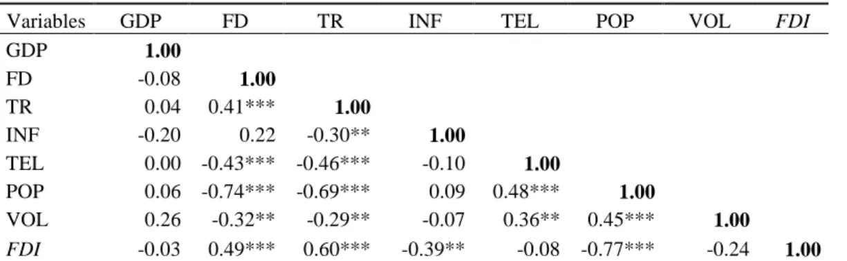
5.1. Correlation Matrix ... 38
5.2. Multicollinearity Statistics ... 38
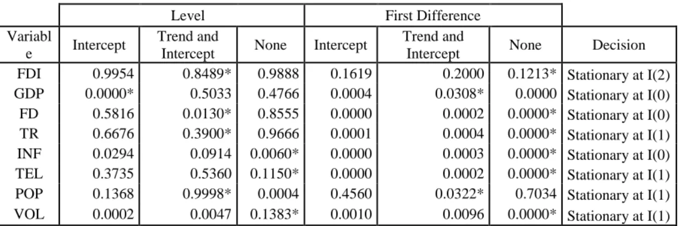
5.3. Stationarity Tests ... 39
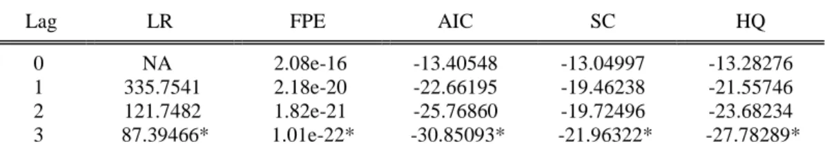
5.4. VAR model, values of information criteria by lag ... 40
5.5. Bounds test ... 41
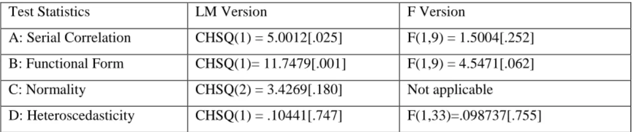
5.6. Diagnostic Tests ... 41
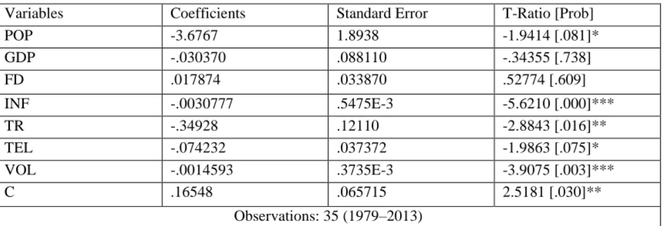
5.7. Long-term estimations of FDI inflows ... 42
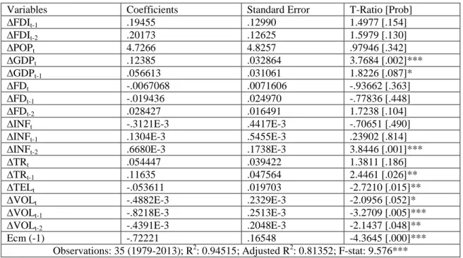
5.8. Short-term estimations of FDI inflows ... 45
6. CONCLUSION ... 48
LIST TABLES
Table 1 - Researched Papers with Independent Variables Statistically Significant with
FDI ... 22
Table 2 - Expected signs on the coefficients, regarding their influence on Brazilian FDI inflows ... 31
Table 3 - Correlation matrix between variables ... 38
Table 4 - Multicollinearity issues between variables ... 38
Table 5 - P-values of the ADF unit root test ... 39
Table 6 - P-values of the PP unit root test ... 39
Table 7 – VAR model, number of lags defined through the information criteria ... 40
Table 8 - Bounds test for cointegration analysis ... 41
Table 9 - Diagnostic tests for ARDL estimations... 41
Table 10 - Long-term estimations of FDI inflows ... 43
Table 11 - Short-term estimations of the FDI inflows based on AIC... 45
Table 12 – FDI inflows in Brazil detached by industries from 2006 until 2014. ... 56
Table 13 - Descriptive statistics ... 56
Table 14 - P-value of the PP unit root test of the POP variable in the 2nd difference .... 57
Table 15 - P-value of the ADF unit root test of the FDI variable in the 2nd difference .. 57
Table 16 - Bounds test for cointegration analysis with 1 lag ... 57
Table 17 - Bounds test for cointegration analysis with 2 lags ... 57
Table 18 - Diagnostic tests for ARDL estimations with 1 lag... 57
Table 19 - Diagnostic tests for ARDL estimations with 2 lags ... 57
Table 20- ARDL estimations of the FDI inflows based on AIC ... 59
LIST OF FIGURES
Figure 1: Evolution of Brazilian Inflation from 1976-2014. ... 24Figure 2: Evolution of Brazilian FDI Inflows from 1976-2014 ... 26
1. INTRODUCTION
Several studies have focused on the impact that macroeconomic and financial variables might have on the foreign direct investment (FDI) of a specific country. Many have been establishing some kind of relationship between the exchange rate volatility and its influence on FDI. However, there is no consensus regarding how significant and what kind of influence (negative or positive) this variable has on alluring or keeping away foreign investors from investing in a specific country.
FDI is taken as an important contribution and fundamental component for a country’s economic growth (Borensztein, De Gregorio, & Lee, 1998; Alfaro, Chanda, Kalemli-Ozcan, & Sayek, 2004; Azman-Saini, Law, & Ahmad, 2010; Bibi, 2014). Its motivations as regards to the host country can be varied, from creating, increasing and improving employment to technology and know-how transfers, or even looking just for the right financial resources.
Throughout the last decades Brazil has been seen by foreign investors as an emerging country with many opportunities to invest, which has been making FDI a significant playmaker on the country’s industrialization and development. Brazilian economy has been suffering from many economic and structural policies, which have been affecting not only their exchange rate flows and regimes, but also their FDI inflows. From the time when liberalization and open trade policies took Brazil, in the 90’s, it was noticeable its effects on the massive growth of FDI inflows, and on general economic growth as well. With all the implementations Brazil took, it was estimated that 80% of the world’s 500 major firms were investing, in FDI terms, into Brazil (Kang & Shou-Ronne, 2012).
Ever since the collapse of the Breton Woods agreement, and the beginning of a fluctuating exchange rate system, the unexpected and unpredictable variation that could come from any currency turned foreign investors much more focused and worried about the potential losses they could take with such volatility.
To best of our knowledge, despite the increase on the studies regarding the relationship between exchange rate volatility and FDI, Brazil has not been very taken into account when analyzing that impact through a time series econometric analysis. This study aims to contribute with not only, a specific analysis of this relationship, but also between the inclusion
of other variables that through the years have also been important motivations for foreign investors in other countries. The fact that these relationships are analyzed within a period of economic and fiscal policies changes in Brazil, and also through a very specific methodology that allows estimations in both short and long-term, makes this study a good and original contribution for the existing literature. Therefore the contributions that this study gives to the existing literature are: it relates both FDI and Brazil on a time series analysis (all the papers focusing on this theme were analyzed through panel data methodologies, meaning their estimation are made based on the average of all countries in the sample. Therefore, the time series methodology turns out to better in this case since it reflects the reality of one country); a new relationship is taken into account in this time series analysis on real effective exchange rate volatility and FDI; the methodology that allows a long term and short term estimations on this relationship.
At first, this study takes into account a time series analysis, from 1976 to 2013, with Brazilian data as sample, where the impact of not only exchange rate volatility but also, GDP growth, Population growth, Financial development, Trade openness, Inflation and Informational Infrastructure are measured against FDI inflows. These variables were chosen according to their importance as positive or negative influences on FDI, presented in previous research studies (focused on other countries).
The main motivation for this study is to provide an analysis that can show how foreign investors are thrived to invest in Brazil, taking into account Brazilian macroeconomic and financial variables.
In order to perform the time series analysis, this study uses the AutoRegressive Distribution Lag (ARDL) model as main methodology for the whole analysis. Before hand, are performed the correlation, multicollinearity and stationarity tests, in order to check for any issues that might be able to decrease the adequacy of the model. With the stationarity tests it is found that variables are stationary in different orders, which makes these tests having mixed results. ARDL model can and is the model to use when variables are stationary in different orders. This model covers a cointegration test, diagnostic tests that allow to check if the model is feasible or not (Serial Correlation, Ramsey’s RESET, Normality and Heteroscedasticity tests),
information infrastructure in the long-term (however the last 3 variables with unexpected signs), while in the short-term gross domestic product (GDP) growth, real effective exchange rate volatility, trade openness, information infrastructure and inflation were the ones showing statistical significance (with the last 2 variables having unexpected signs). As regards to the main objective of this study, it is found that real effective exchange rate volatility either in short and long-run affect negatively FDI inflows in Brazil.
The remainder of this study is structured as follows: Chapter 2 presents a detailed review of the literature regarding FDI, exchange rate volatility, and their relationship. Chapter 3 gives a detailed review of literature regarding Brazilian economy, focusing more on its FDI historical values and economic policies with effects on exchange rate regimes. Chapter 4 focuses mainly on data and methodology approaches. Chapter 5 presents the results and their respective analysis. Chapter 6 presents the conclusion with a brief summary of the main findings and suggestions for future research.
2.
LITERATURE REVIEW
2.1. FDI
According to the World Bank, FDI is defined as “the net inflows of investment to acquire a
lasting management interest (10 percent or more of voting stock) in an enterprise operating in an economy other than that of the investor. It is the sum of equity capital, reinvestment of earnings, other long-term capital, and short-term capital as shown in the balance of payments”1.
An even more complete definition of FDI is given by International Monetary Fund (IMF) and Organization for Economic Co-operation and Development (OECD), which state that:” a
direct investor may be an individual, an incorporated or unincorporated private or public enterprise, a government, a group of related individuals, or a group of related incorporated and/or unincorporated enterprises which have a direct investment enterprise, operating in a country other than the country of residence of the direct investor. A direct investment enterprise is an incorporated or unincorporated enterprise in which a foreign investor owns 10% or more of the ordinary shares or voting power of an incorporated enterprise or the equivalent of an unincorporated enterprise. Direct investment enterprises may be subsidiaries, associates or branches. A subsidiary itself is an incorporated enterprise in which the foreign investor controls directly or indirectly more than 50% of the shareholder’s voting power. An associate is an enterprise where the direct investor and its subsidiaries control between 10% and 50% of the voting shares. A branch is a wholly or jointly owned unincorporated enterprise. Once a direct investment enterprise has been identified, it is necessary to define which capital flows between the enterprise and entities in other economies
should be classified as FDI”2
.
Though, despite the definition given by OECD as regards to the direct investment, there is no consensus regarding the control of the minimum 10% shareholding, and countries have different approaches to the criteria used, and limit values (some countries do not even have
limit share for considering a direct investment, instead, they have other measures to analyze it).
For Caves (1974) FDI brings to the host countries many positive effects to their economies, such as technology transfer, managerial skills, know-how, international production networks, etc. However, FDI goes way beyond of promoting growth, technology and education into a country. It has many different types of utility that can serve to a country: develop a country’s infrastructure, rebalance its national budget surplus, mature human capital, finance capital accumulation that could ease imbalances, and even serve as a cushion against any sort of short and long term shocks and economic development. Determinants for alluring FDI are dependent on what each country is able to provide, such as economic and political stability, policies regarding investment incentives (privatization policies, trade policies, tax exemptions/reductions, etc).
FDI is taken into account when foreign investors have one of these 2 strategies: 1st they want to invest in a market with the goal of through lowering production costs, turning their imports from that country less expensive into theirs; 2nd foreign investors are allured by the raw materials and good quality resources that the receiving country has, thus investing in those countries would allow to improve their exports capacities and expand their business.
2.2. Exchange Rate Volatility
Exchange rate volatility (ERV) is defined as a variation of the prices of one currency in terms of another. By depreciating or appreciating the value of a foreign currency, profitability of foreign exchange trades will be affected. Volatility in this case takes into account all the movement and changes that are influential for a depreciation/appreciation of a currency.
ERV started to be subject and field of study majorly since the collapse of the Bretton wood system in the 1970s. Among many fundamental studies and theories, some examples like Lin, Chen, & Rau (2010) and Haile & Pugh (2013) contributed with some of the effects that the exchange rate volatility has in the macroeconomic world (for instance, interest rate or inflation became much more volatile). Exchange rate volatility became a huge player also for financial markets, trading and speculation activities were rising, and becoming object of a lot of research.
As a result of the abandonment of the fixed exchange rate regime, international investment flows of capital became much higher (as well as international trade and other foreign exchange transactions), and despite the growth, markets were insecure regarding the risk foreign investors may take to put their money abroad (Chowdhury & Wheeler, 2008).
As volatility is referred to an unpredictable and unobservable pattern, foreign investors became more aware and tried to get much more information in order to be possible to dispend less transaction costs by hedging against exchange rate volatility risk. By hedging against exchange rate volatility, investors have to take into account that these methods bring with them some drawbacks. For example, when dealing with forward contracts or some type of foreign business contract in which, one party could immediately convert its money to the foreign currency to avoid negative consequences from volatility. However, the drawback of this hedging strategy is that, the money invested and converted in the foreign currency, is no longer useful for future domestic opportunities. Despite the hedging strategies against ERV, there is always (like in any other investment) a sunk cost to be endured, and for foreign investors, this is as always a huge disincentive for them to invest abroad, especially with a huge uncertainty that ERV brings.
2.3. Theoretical Approach
There are some theories that have been developed through the years, and that have been searching for a certain degree of relationship between FDI and its determinants (one of them, the exchange rates movements).
Many studies have been giving theoretical and empirical examinations, regarding the relationship between exchange rates and FDI. However, there is no consensus on the nature of this relationship, because the large majority of the studies are made with different time intervals, different countries, different data (like the determinants and the models that are used) or even through different methodologies. It depends also, on the motivations of each study and its purpose.
Theories3:
Standard option theory: if there are fixed costs in the acquisition of a firm, firms tend to delay their investments (for example in acquisition processes) when they are facing higher exchange rate volatility. Depending on how the home currency equivalent of expected future cash flows from the target firm is correlated with other assets in the acquiring firm’s portfolio, high exchange rate volatility may have a positive or negative effect on the investment decision (di Giovanni, 2005).
Trade theory: FDI may be higher in countries experiencing uncertainty regarding the exchange rate because such uncertainty acts as a barrier to trade. Multinationals engage in FDI to avoid uncertainty affecting the price of their traded goods as the exchange rate fluctuates. Thus, multinationals increase their FDI to substitute for lower trade volumes in markets associated with higher volatility (Goldberg & Kolstad, 1995). Also, cross-border investment may be a substitute for trade when tariffs or other barriers prevent the free flow of goods (Russ, 2007).
Imperfect Capital market theory: Changes in relative wealth affect the bids these firms make, when the purchase of an asset requires funds that are generated within the firm. Thus, depreciation in the host country, by making the relative wealth of foreign investors increasing (outbidding domestic investors) and lowering the investment cost of capital (that is launched in the domestic currency), encourages FDI into that country (Itagaki, 1981; Cushman, 1985; Froot & Stein, 1992; Klein & Rosengren, 1992; Kiyota & Urata, 2004).
Traditional theory: If a country’s asset is seen as a claim to a future stream of its currency denominated profits, and if profits will be converted back into the domestic currency of the investor at the same exchange rate, the level of exchange rate does not affect the present discounted value of the investment (Blonigen, 1997).
Real options theory: the flexibility of the option value that a firm has in delaying an investment decision in order to obtain more information about the future. For a firm to raise profits from FDI activities, it must be taken into account the different types of FDI and its timing. Therefore, the impact that the exchange rate uncertainty might have on firm’s decision to invest, is ambiguous. In the case of a risk averse firm, whenever the
3For more theories regarding other aspects on FDI please check the Internalization theory with fundamentals
from Coase (1937) and Hymer (1960) studies, and the Eclectic theory of international production with fundamentals from Dunning (1980, 2001) studies.
exchange rate uncertainty becomes higher, a market-seeking firm tends to delay its decision to invest, however if it is an export-substituting firm, the decision is to increase its FDI activity (Dixit & Pindyck, 1994).
2.4. Effect of Exchange Rate Volatility on FDI
When it comes to the relationship between exchange rate volatility and FDI, the studies do not get to a consensus, and thus, there is not a proven concept that can make an analysis correct or incorrect. Some studies have shown that, the degree of the impact of exchange rate volatility on FDI is different across industries (Froot & Stein, 1992), and across countries (Ogunleye, 2005), different by motive of the investing firm (Chen, Rau, & Lin, 2006; Phillips & Ahmadi-esfahani, 2008), or even across different time intervals (Wakelin & Gorg, 2002; Schmidt & Broll, 2009).
Trade is an element that has been reason for many studies similar to the ones regarding the relationship between exchange rate volatility and FDI, in order to see the impact that it suffers from exchange rate volatility. Those studies have emerged, they show how exchange rate volatility may impact in a positive or negative fashion on trade flows depending on the assumptions employed with respect to the nature of the response to risk, the availability of capital, the time horizon of the trader and whether the firm is a manufacturer or a non-manufacturer (McKenzie, 1999).
Some studies show that firms who engage in FDI as a substitute for exports, will accelerate their FDI when faced with exchange rate volatility, while those firms seeking new markets for their products will delay their FDI. Thus, the relationship is country and industry specific (Chowdhury & Wheeler, 2008). Multinational firm’s response to exchange rate volatility differ depending on whether the volatility arises from shocks in the firm’s native or host country (Russ, 2007).
2.4.1. Positive Relationship between FDI and Exchange Rate
Volatility
Itagaki (1981) states that when the home currency is expected to depreciate, the multinational enterprises increase foreign sale, and decrease import of foreign intermediate goods. This implies that the balance of trade of the home country is improved simply by anticipation of depreciation of the home currency. However regarding the exchange rate volatility, the author concludes that it may incite a firm to invest abroad as a way of hedging against a short position in its balance sheet.
Cushman (1985) paper concentrates on short-run volatility, using a time series data of the US considering bilateral direct investment flows to 5 industrialized countries, and an unquestionable innovative methodology that permitted the results to be completely accurate, concluded that the effect of a risk-adjusted expected foreign currency appreciation lowers foreign capital cost, which consequently stimulates FDI. Also this study showed evidence that against exchange rate risk, a MNE reduces its exports, but increases its foreign capital input and production, which compensates foreign currency reserves and is observed a consequent growth in FDI.
Goldberg & Kolstad (1995) concentrate on the long-run exchange rate volatility, using quarterly US bilateral FDI flows with Canada, Japan, and the UK, it argues that depending on different behavioral assumptions and on the types of shocks that the economy takes exchange rate volatility might (or not) affect FDI. For instance, Goldberg & Kolstad (1995) found that, the exchange rate volatility determines the production location as a response to an increase in production capacity (which might affect the type of investment that is made from a MNE). Thus, even if investors are risk averse but production is assumed to be a fixed factor, there is no statistical relationship between exchange rate volatility and FDI. However if production reacts according to exchange rate volatility, then this relationship becomes statistically significant and positive (an increase in the foreign money supply increases demand, while raising prices, leads to a short term real appreciation of foreign currency).
Chowdhury & Wheeler (2008) study focused on the impact that exchange rate volatility has on FDI from Canada, Japan, UK, and US. Their study followed a VAR (Vector Autoregressive) model and found statistically significant evidence of a positive impact between exchange rate volatility and FDI in each of the 4 countries under observation.
Takagi & Shi (2011) using a panel data of Japanese investment in 9 Asian economies found a positive relationship with exchange rate volatility. Despite financial flows and exchange rates seemed to be affected by the Asian financial crisis, results were robust and had the expected outcomes, where by following Itagaki (1981) and Cushman (1985), justified their result (regarding the relationship between FDI and ERV), with the will of foreign investors to promote FDI as a substitute for exports.
2.4.2. Negative Relationship between FDI and Exchange Rate
Volatility
Campa (1993), Bénassy-Quéré, Fontagné, & LahrÈche-Révil (2001), Kiyota & Urata (2004), and Ogunleye (2005) find negative impact of exchange rate volatility on FDI (specially from developed to developing countries, in the case of the Bénassy-Quéré et al. (2001) study), which is exactly the opposite from the previous referred studies. Ogunleye (2005) study has a contrast and unexpected results, where the findings for Nigeria and South African economies differ. At first in Nigeria exchange rate volatility as it is expected, has negative statistical significance on FDI, however, in South Africa the same does not happen, not only the relationship is positive but also, is not statistically significant. Campa (1993) found that the volatility in exchange rate affects in a negative way the US’s FDI. Kiyota & Urata (2004) observed that in Japan, the depreciation of the yen enhanced FDI while the increase in exchange rate volatility discouraged FDI at both aggregated and disgreggated industry levels (stating that an overvaluation of a country’s currency discourages its inward FDI).
Xing (2006) also finds negative impact, assuming that for firms that are risk averse, a higher degree of exchange rate risk will reduce inward FDI into the host country.
Wang (2013) determines that higher exchange rate volatility lowers investment projects such as FDI, because considering that investors are risk averse their certainty of return decreases as the risk increases.
2.4.3. Other Results and Perspectives
Aizenman (1992) showed that in a flexible exchange rate regime the correlation depends on the nature of the shocks. However this study followed the assumption of risk neutrality, which means that foreign investor did not change behavior according to the degrees of risk. The study concluded that if the dominant shocks are nominal, there is a negative correlation, whereas if the dominant shocks are real, there is a positive correlation between the level of investment and exchange rate volatility. Thus, while for real shocks the higher exchange rate volatility, the higher FDI, for nominal shocks, the higher the volatility the lower the FDI.
Blonigen (1997) suggests that FDI flows into an economy can increase with exchange rate depreciation if domestic and foreign firms are bidding for firm-specific assets since these assets generate returns in currencies other than the one used to purchase them.
Wakelin & Gorg (2002) examines the impact of the exchange rate volatility between US FDI flows and 12 developed countries, from 1983 to 1995. They found a negative relationship between US inward investment and appreciation in the dollar. However, when it comes to US outward investment, there is a positive relationship with an appreciation in the host country’s currency. Despite all the findings regarding exchange rate volatility relationship with FDI, this study found no significant relationship as for inward or outward FDI.
Xing (2006) study along with the analysis regarding the impact of real exchange rates on Japanese FDI in China, argued that the depreciation of the Yuan substantially enhanced inflows of direct investment from Japan (negative correlation between exchange rate and FDI), and that the response of FDI to change of the real exchange rate is elastic.
According to Arize, Osang, & Slottje (2008), increases in the real exchange rate volatility, exert a significant negative effect upon export demand in both the short and the long run.
Schmidt & Broll (2009) study analyzed empirically the impact of exchange rate uncertainty (using two different measures for the estimation of the exchange rate volatility) on US FDI from 1984 to 2004. Using as benchmark of real exchange rate volatility the standard deviation of annual percentage changes, the study found negative statistical significance effect on US FDI outflows for the majority of the industries (Manufacturing, Food, Chemicals, Primary and Fabricated Metals, Electric Machinery, and Depository institutions). The alternative measure of real exchange rate volatility defined as unexplained part of real exchange rate
volatility, showed a negative effect on Manufacturing industries regarding US FDI outflows and positive effect on Nonmanufacturing sectors.
Concer, Turolla, & Margarido (2010) models the FDI outflows from Brazil with quarterly observations between 1995 and 2010 and found that, the strong exchange rate in Brazil is often blamed for forcing companies to invest abroad, however there is no statistical significant relationship between the level of foreign exchange rate and the Brazilian FDI outflows.
Lin, Chen, & Rau (2010) show that the nature of the relationship between FDI and exchange rate volatility depends on the motive behind FDI. They show that firms who engage in FDI as a substitute for exports will accelerate their FDI when faced with exchange rate volatility, while those firms seeking new markets for their products will delay their FDI.
Most of the studies ignore the financial development on the country in analysis, and regarding that, there is Khraiche & Gaudette (2013) whose results show that the impact of exchange rate volatility on FDI in economies with lower financial development tends to be significant and positive, but the effect is not significant for countries with greater financial development. Thus, when a multinational makes a decision to engage in FDI to alleviate the costs of exchange rate volatility, its decision should depend on the level of financial development in the receiving country.
2.4.4 Impact of other Control Variables on FDI
On analyzing the general impact that exchange rate volatility may have on a country’s macroeconomic level, some variables will be tested as they were experienced by other researches. Since FDI suffers big influence from a lot of determinants, to understand its full impact on what foreign investors really take into account, not only the impact of the ERV will be assessed, but also, other important explanatory variables that might have the same or even more influence on FDI.
These researches usually tend to test on specific economies, dates or/and industries. So if the studies differ on some variables or measurements, such as the country itself, they can’t justify
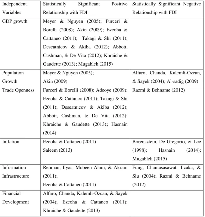
Briefly, based on the reviewed literature (please see also Table 1) and on the available data for an annual analysis in the specific observation period that this research is focused on, to analyze the full impact that FDI inflows in Brazil suffer from other variables, it is reached the conclusion that this study will be focusing on the following variables: GDP growth, population growth, information infrastructure, REER volatility, trade openness, financial development and inflation. Even though these variables might not be significant in some papers, when taking into account the Brazilian economic situation on this specific observation period, it is firmly believed that for the case of Brazil these variables are a matter of highly importance.
Table 1 - Researched Papers with Independent Variables Statistically Significant with FDI
Independent Variables
Statistically Significant Positive Relationship with FDI
Statistically Significant Negative Relationship with FDI
GDP growth Meyer & Nguyen (2005); Furceri & Borelli (2008); Akin (2009); Ezeoha & Cattaneo (2011); Takagi & Shi (2011); Deseatnicov & Akiba (2012); Abbott, Cushman, & De Vita (2012); Khraiche & Gaudette (2013); Mugableh (2015) Population
Growth
Meyer & Nguyen (2005); Akin (2009)
Alfaro, Chanda, Kalemli-Ozcan, & Sayek (2004); Al-sadig (2009) Trade Openness Furceri & Borelli (2008); Adeoye (2009);
Ezeoha & Cattaneo (2011); Takagi & Shi (2011); Deseatnicov & Akiba (2012); Abbott, Cushman, & De Vita (2012); Khraiche & Gaudette (2013); Hasnain (2014)
Razmi & Behname (2012)
Inflation Ezeoha & Cattaneo (2011) Saleem (2013)
Borensztein, De Gregorio, & Lee (1998); Hasnain (2014); Mugableh (2015)
Information Infrastructure
Rehman, Ilyas, Mobeen Alam, & Akram (2011);
Ezeoha & Cattaneo (2011)
Fung, Chantasasawat, Iizaka, & Siu (2004); Razmi & Behname (2012)
Financial Development
Alfaro, Chanda, Kalemli-Ozcan, & Sayek (2004); Ezeoha & Cattaneo (2011); Khraiche & Gaudette (2013)
3. BRAZIL
The sample in this research is the Brazilian FDI inflows. Brazil was the chosen country due to the following reasons:
There is no study that establishes and contributes to this relationship, as regards to the period of study, the methodology used and all the gathered data combined;
Brazil has been suffering a lot, within the period of analysis, from economic and fiscal policies changes, making it a good sample to be subject of analysis for this topic.
3.1. Period 1970-1980
Considering the period of analysis in this study, and beginning in the 70’s Brazil, this decade is registered as having an impressive economic growth, mainly due to 2 facts, on one hand the fact that most of the countries of Latin America absorbed the excessive liquidity that the U.S., Japanese and European markets were having. On the other hand, the fact that with the end of World War II, the countries that made part of it were struggling to recover their economies, thus in order to fulfill their need for economic growth, they started to develop interest on foreign countries, and since Brazil had implemented a liberal policy regarding foreign capital, where there were not any tariffs or barriers for imports, they took the advantage of it (Gregory & Oliveira, 2005).
With this policy of import substituting industrialization, Brazilian economy wanted to become less dependent on commodity-based exports and more allured for investments inwards, in order to develop its infrastructures and industries.
To have a general idea, the average FDI inflows Brazil was getting between 1950 until 1969 were about $120million, while for the 70’s the amounts were averaging $1342million. The same happens with FDI outflows, Brazil was not practically investing abroad between 1950 and 1969, with an average of outflows hanging around the $3million, right after the beginning of the 70’s Brazilian FDI outflows fired up to some impressive numbers, a mean annual inflow of FDI of $72 million.
3.2.Period 1980-1990
A major increase in interest rates were starting to be felt worldwide, foreign investor’s confidence decreased, causing a decrease in foreign investment, which made both external debt and inflation increasing and forcing the Brazilian economy to implement austere regulations. Later, Brazil adopted through economic measures a very strict plan in order to reach monetary stabilization (Loman, 2014).
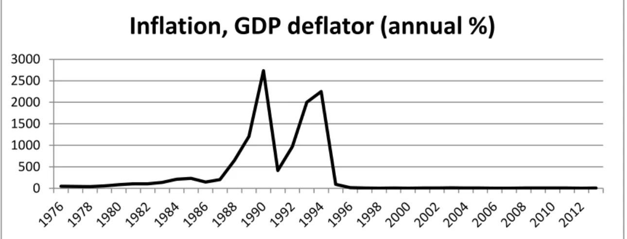
Along with this economic and political turbulences, military dictatorship that had been ruling Brazil since the 1960’s, was forced to leave in 1985, as democratic ideals stepped into the scene. Despite this change in the Brazilian politics, the former bad practices with budget deficits being financed, devaluations that retracted Brazilian economy, the non-stop growing inflation (please see Figure 1), and the difficulty on contradicting the events worldwide mainly regarding interest rates, led the country to a hyperinflation crisis (Loman, 2014).
Figure 1: Evolution of Brazilian Inflation from 1976-2014. Source: World Bank
3.3.Period 1990-1999
In the 90’s, government policies were aiming to a new direction, with a series of fiscal and economic reforms, leading to trade liberalization, deregulation, privatization and the establishment of a legal and structural framework to promote foreign investment (Christiansen, Oman, & Charlton, 2003; Gregory & Oliveira, 2005; Concer et al., 2010; Loman, 2014; Weisbrot, Johnston, & Lefebvre, 2014). Regarding FDI inflows, the goal was combining policies applied to allure foreign investors and industrial technology on the different sectors. 0 500 1000 1500 2000 2500 3000
In 1994, in order to stabilize the Brazilian economy, the Real Plan was introduced, with the main goal of giving a sustainable reduction in prices (after 3 decades of consecutive growing inflation) in order to stabilize the domestic currency in nominal terms. As part of the Real Plan, a new currency was introduced (the Real) substituting the short-lived Cruzeiro Real, with a conversion rate 1=2.75 respectively. The Central Bank decided to peg the Real currency to the Dollar (crawling peg) making R$1.00 valuing as much as US$1.00. This crawling peg4against the dollar as a nominal anchor was overvalued, which made imports cheaper. Monetary policies were established which included a fiscal contractionary policy that caused an increase on the interest rates (contributing to a deterioration of the fiscal accounts), and the immediate depreciation of the Real (Agénor, Hoffmaister, & Medeiros, 1997).
In the same year the Real Plan was introduced, a process to achieve an agreement of a single common market (between Brazil itself, Paraguay, Uruguay and Argentina) was taking place. This regional-integration process Mercosul in Brazil’s point of view was an important device to expand the liberalization trade policy reform that was taking course, thus gaining more capacity to open the Brazilian market to outside investment with the advantage of increasing domestic competition (Christiansen et al., 2003).
Right after the adoption of the currency Real, in 1995 the exchange rate system started to be subject to an exchange rate band, responding to market factors and still leaving control to the Central Bank, fluctuating with the Dollar within certain limits that were continuously changing - The first Band was set on March 6th 1995 at R$0,86-R$0,90 per U.S. Dollar (Agénor et al., 1997).
When selecting an exchange rate regime for a country, some considerations have to be made, bearing in mind the consequences that it can bring with it. Capital flows, inflation, balance of payments, as well as other macroeconomic essentials, suffer a direct impact on this regime choice. Tendentiously a country chooses its exchange rate regime in order to establish short and long term economic stability, growth and financial development. It truly depends on the situation of the country, which means is not an automated process that regardless the type of situation the country is dealing with, there will be a proper and consensual exchange rate regime. Therefore an exchange rate regime usually is followed by a macroeconomic and
Along with the implementations of the new currency Real, Brazil’s FDI inflows started to have more diversified foreign investors, targeting to different industrial sectors and to much larger amounts of investment. Brazil has become an open economy, with low tariffs and practically no barriers to imports. As a consequence of this trade liberalization, Brazil was strongly affected by its enormous gap, regarding the amount of trade deficit (Gregory & Oliveira, 2005).
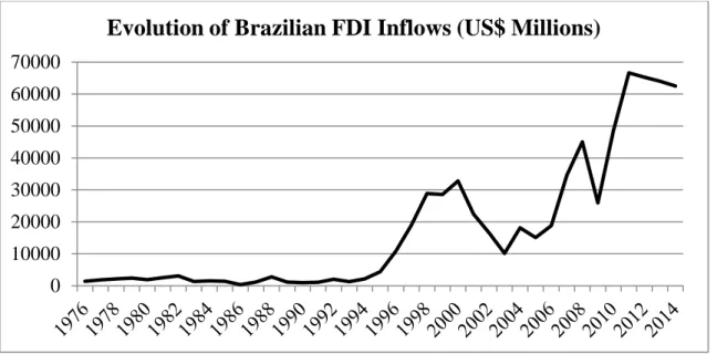
In 1999 with the Russian and Asian crises (that were taking course since 1997) that were weakening the international financial markets, its capital flows were disappearing from their invested markets which consequently brought huge losses to Brazilian economy and its FDI inflows, as it is possible to observe in Figure 2 (Gregory & Oliveira, 2005).
Figure 2: Evolution of Brazilian FDI Inflows from 1976-2014. Source: CBB
Whenever is necessary, central banks can buy or sell their own currency reserves in order to stabilize the local economy. This can happen also when international trade and foreign investments become unpredictable due to the high uncertainty in the exchange rate markets. So, with the 3 decade of consecutive growing inflation, which was causing high money supply for the reason that with the local currency value high, foreign goods will seem a lot cheaper compared to the domestic ones, which stimulates imports and reduces exports (since the local goods will seem more expensive to foreigners).
At the same time along with the liberalization policy, essentially on import tariff reduction, the exports could not keep up with the amount of imports, which consequently turned the Brazilian trade balances into a huge trade deficit. Since the central bank was being pressured
0 10000 20000 30000 40000 50000 60000 70000
to intervene in order to reduce inflation, and to respond to the financial crisis occurring in Asia and Russia, the decision was to implement inflation targeting policy (with the central bank commitment to lower money supply and raise interest rates, thus stabilizing the Brazilian economy) and a rearrangement of the floating exchange rate system into an independent one (Gregory & Oliveira, 2005).
Why did Brazil need to arrange its exchange rate regime? First of all, in this new independent floating exchange rate regime the exchange rate value and as a result the currency value, is determined through the supply and demand relative to other currencies. It is all set in the FOREX market, and there is no official foreign exchange market intervention on the side of the monetary authorities. So, in order to gain a higher competitiveness with the freedom of financial flows in the Brazilian market, since Real’s value is high, the demand for it will decrease, and consequently its value will immediately decrease causing a depreciation, making imported goods more expensive and stimulating demand for the local ones, thus resulting on an equilibrium between the internal and external balance.
3.4. Period 1999-2013
Quickly Brazil noticed its economy stabilizing, the return of big amounts of FDI, and gaining once again confidence in their markets, through the stabilization of the currency (please see Figure 3) and the reduction of the fast growing paced inflation. Despite the consequent high devaluation that occurred right after the change on the exchange rate regime, with the privatization policies, FDI was responding well, where many opportunities were taken at that time from foreigners to acquire assets in the Brazilian economy.
100,00 200,00 300,00 400,00 500,00
Holland (2006) argues that the exchange rate and interest rates behavior in Brazil since 1999, with the introduction of the floating exchange rate regime and the inflation targeting policy, made Central Bank less worried about exchange rate dynamics as much as inflation, since it was still not totally at the values Brazil needed it to be.
In 2001 some events like the New York Stock Exchange fall, big well-known MNE declaring bankruptcy by being accused of fraud, and the fear of terrorist attacks that were hovering on the world population, contributed for a big drop on global FDI values (Gregory & Oliveira, 2005). Together with the reduction on privatization program values, the energetic crisis and the instability caused by the approaching elections Brazil suffering losses of more than 30% (from more than US$32 billion to around US$ 22 billion), which was still below the average worldwide 40% drop.
In 2002 with the uncertainty around the presidential elections, and the suspicions that the government could cause radical changes in Brazilian economic policies, FDI values lowered even more (please see Figure 2), along with a big depreciation in the Real currency.
In 2003, the new government (Partido dos Trabalhadores) and president (Lula da Silva) took possession. Since this party had been showing negative perspectives regarding the Real Currency Plan, foreign investors were afraid that Lula could default on Brazil’s debt, however, the new government did not make any radical changes as the markets and MNE were expecting, instead, they compromised on reducing country’s risk and on strengthening Real currency’s value (Loman, 2014).
Until 2006 FDI values were left stagnated at the same level, however a progress was being felt with a slow recovery of the Real currency’s value against other foreign currencies that were more relevant for the Brazilian market, coming close to its previous value (on the first quarter of 2002) in 2005.
In 2008, Brazil was in a very good position, where exports were doing great and the capital flows were proportionating a balanced trade surplus, FDI was improving its values, and the Real currency was behaving formidably with almost the double of the value that it had back in 2002 and 2003 compared to the US Dollar. With the financial crisis, FDI and the Real value had a temporary breakdown, but since the removal of some restrictions regarding the floating exchange rate system such as taxes on portfolio inflows or limitations of capital inflows, immediately in 2010 gained a strong position with a big increase in their values, even more
than before the crisis. It is fair to say that the financial crisis impact worldwide was not felt in the same proportion by Brazil, in fact, only in 2 quarters of 2008 there was less international capital flowing than the usual. As part of that slowdown, global demand for Brazilian exports decreased with a weaker external credit making contribution for it, however in 2009 Brazil rapidly showed its ability in recovering their economy and handling with the slump.
With the high economic growth that Brazil has been able to produce over the last years, inflation has been in a constant rise since 2011, which led the Brazilian government take measures to calm the growing economy with an inflation targeting policy. Since then. the high inflation along with the persistent deterioration being felt in other economies by the financial crisis, have been causing a deceleration on Brazil’s economic growth.
From 2010 until 2013, due to the high level of growth of imports, FDI and other foreign capital inflows, Real’s currency tended to improve its value and appreciate (essentially in 2010 and 2011) against other currencies. However with the Real’s appreciation alongside with the growing inflation, made Brazilian companies (essentially the manufacturing ones as it can be seen in Table 10 on the appendix) lose competitiveness against foreign companies, leading the Brazilian government to raise taxes on foreign capital inflows and to manipulate their currency value in FOREX markets. The so called “currency war” occurred when some countries led their own currencies to depreciate more than what they were really valuing at that time. The goal was to depreciate their currencies at a value that could not only still be competitive with others, but also increase by a big amount their exports in order to be much more competitive (Loman, 2014).
4. DATA AND METHODOLOGY APPROACH
The observation period spans between 1976 and 2013. The reasons for this particular period are the fact that, is the period for which all data are available and where it is possible to see Brazilian economy suffering from a lot of global and national scale events such as, changes in exchange rate regime, financial crisis, changes in monetary and fiscal policies. Since the period that is going to be analyzed will be 38 years (38 observations) and the majority of the variables only have available data on an annual basis, the data frequency provided for analysis is going to be annual.
When measuring the impact of exchange rates movements on Brazil’s FDI, there will be an analysis of FDI inflows, in order to better understand the impact that it takes on the will to invest by foreign investors in an emerging market like Brazil. FDI flows were extracted from the Central Bank of Brazil. The unit of measure, regarding currency units, is the US Dollar for the Brazilian FDI inflows, and all the other explanatory variables that require currency units.
In order to understand and have a general idea of the volatility of the exchange rate regarding the Real currency, this study will focus on the volatility of the real effective exchange rate.
4.1. Model Specification and Control Variables
In order to investigate the impact of exchange rate volatility on FDI inflows in Brazil, there will be estimated an equation where FDI inflows in Brazil is reflected as a function of the following variables: GDP growth, real effective exchange rate volatility, financial development, trade openness, inflation, information infrastructure, and population. All the previous variables are regarding Brazilian economy. The data for determining the most influent variables is chosen according to the characteristics that Brazil possesses that create more impact in their own economy. Brazilian FDI inflows data were collected from the Central Bank of Brazil database, and as a dependent variable it is used as a ratio between FDI in time t to GDP in time t.
FDIt = β0 + β1VOLt + β2GDPt + β3FDt + β4TRt + β5INFt + β6TELt + β7POPt + c (1) , where β0 is the intercept and βi (i=1,2,3,4,5,6,7) represents the coefficient for each of the independent variables. FDI is the foreign direct investment inflows into Brazil, VOL is the real effective exchange rate volatility (REER), GDP is the GDP growth, FD is the financial
development, TR is the trade openness, INF is the inflation, TEL is telephone mainlines (a proxy used for information infrastructure), POP is the population growth. C is the constant term of the regression.
For a better analysis, all variables are expressed as ratios related to GDP (FDI, trade openness, financial development), growth rates (inflation, information infrastructure, population), or in variation rate (real effective exchange rate volatility). All the variables with the exception of REER volatility were extracted from the World Bank database, while REER volatility variable was extracted from the OECD database.
In the equation 1, the time subscript t is not omitted, due to an analysis on a specific time horizon. Within this equation an error term is included. This formula generalizes the effects of each determinant (through their respective aggregates) on the time series analysis, allowing an analysis of the wide impact that each independent variable has on the dependent one, giving a macroeconomic perspective from the foreign investors point of view. However, some effects may be due to specific sectors, firms or industries, and we are unable to find the degree of impact that it took in the Brazilian FDI inflows. Also, other effects that might be considered insignificant, don’t exactly mean that foreign investors don’t care about that determinant when looking to invest in Brazil, only that they don’t look at it on a generalized form. Thus, with the microeconomic perspective being ignored in the methodology, foreign investors restrict their investments to a more limited point of view.
As the main purpose of analysis, the hypothesis that this research aims to address and give answer, taking into account the reviewed literature, is that, the exchange rate volatility has significant negative impact on Brazilian FDI inflows in both short term and long term.
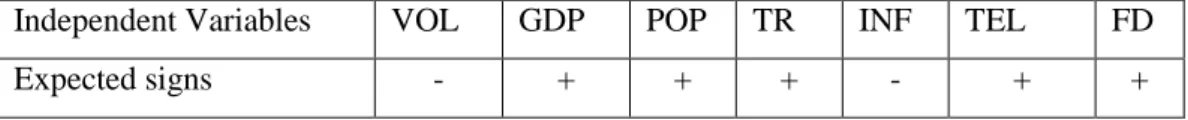
Regarding the influence each of the determinant may have on Brazilian FDI inflows and based on the majority of the results given by the reviewed literature (please see Table 1), their coefficients are expected to have the following signs:
Table 2 - Expected signs on the coefficients, regarding their influence on Brazilian FDI inflows
Independent Variables VOL GDP POP TR INF TEL FD Expected signs - + + + - + +
Below, is explained which are the foundations of each of the independent variables:
Exchange Rate Volatility – In this study REER is defined as the relative consumer price index (through following the Law of One Price (LOP)5 and Purchasing Power Parity (PPP)6). The real effective exchange rate volatility is estimated following Wakelin & Gorg (2002), Furceri & Borelli (2008) and Schmidt & Broll (2009) measurement, through the annual standard deviation of the monthly changes in the REER. Other alternatives to measure volatility, would be the Generalized Autoregressive Conditional Heteroscedasticity (GARCH) developed by Bollerslev (1986), which is the improved version of the Autoregressive Conditional Heteroscedasticity (ARCH) developed by Engle & Granger (2007). The standard deviation as an unconditional measure, does not condition upon the information that is available today, it simply takes into account the past average of historical observations, therefore it ignores stochastic problems through time. However the volatility of the exchange rates in this study is aimed to explore the existence of long and short-term connection with FDI in the past, which for the simplicity of the volatility measure, allows this variable to be used through the unconditional measure. Taking into account the Brazilian currency’s development through this observation period and its possible influence on a macroeconomic level, the variable REER volatility is expected to have a negative relationship with Brazilian FDI inflows. GDP Growth – Emphasized by the majority of the papers as an important variable (
Furceri & Borelli, 2008; Akin, 2009; Mugableh, 2015) , represent as percentage, the country’s economy progress from t-1 to t, as the progress in the size of the local economy and their wealth produced compared to the year before, can be considered as the country’s market economic potential. Since the higher the market potential the greater the market receptiveness for FDI, GDP growth is expected to have positive influence on Brazilian FDI.
Population – This variable is used as a market size estimator, where its true intent is to analyze the amount of Brazilian FDI inflow is dependent on the variation of the size of the economy. With a growing population and economy, it may reach a level which guarantees the exploitation of economies of scale, making a country targeted for FDI (Alfaro,
5States that the relative cost of producing traded goods has to be the same, when measured in a common
currency in both home and foreign countries, in order to don’t give any arbitrage opportunities to any of the involved parts (this is done by adjusting the nominal exchange rate to reflect in the prices or costs in the traded goods in both home and foreign country).
6Determinates that an exchange rate adjusts the price or cost of an identical good in 2 different countries, making
Chanda, Kalemli-Ozcan, & Sayek, 2004; Meyer & Nguyen, 2005; Akin, 2009). This variable constitutes as a percentage, the population growth from t-1 to t, thus since the higher population growth (consequently the market size and its potential), the higher the interest of foreign investors on that economy, this variable is expected to have positive influence on Brazilian FDI inflows.
Openness to Trade – This variable is estimated as the ratio of the sum of both exports and imports with GDP at time t (Furceri & Borelli, 2008; Takagi & Shi, 2011; Abbott et al., 2012; Deseatnicov & Akiba, 2012; Khraiche & Gaudette, 2013), representing the degree of “economic freedom” that a country has to receive foreign investment, thus the expected influence on Brazilian FDI inflows is positive.
Informational Infrastructure – This variable takes into account that for a country to allure foreign investment, it must have fine infrastructures in order to satisfy production, efficiency and all the necessary requirements for the specific foreign firm/investor. Following Akin (2009), Ezeoha & Cattaneo (2011), Rehman, Ilyas, Mobeen Alam, & Akram (2011) and Abbott et al. (2012) this variable is estimated as percentage of growth from t-1 to t, using as a proxy, the number of telephone mainlines. It is expected to have positive relationship with Brazilian FDI.
Inflation – This variable represents as percentage, the degree of macroeconomic stability in price terms from t-1 to t, where higher inflation reflects a higher macroeconomic instability (Borensztein, De Gregorio, & Lee, 1998; Furceri & Borelli, 2008; Ezeoha & Cattaneo, 2011). Since macroeconomic instability provokes foreign firms to retract their will to invest outboards, inflation is expected to have a negative relationship with Brazilian FDI.
Financial Development – This variable represents the financial resources provided to the private sector, such as through loans, purchases of non-equity securities, trade credits and other accounts receivable that establish a claim for repayment. Following Alfaro, Chanda, Kalemli-Ozcan, & Sayek, (2004) and Ezeoha & Cattaneo (2011), financial development is measured through the ratio of broad money supply to GDP. Since financial development plays an important role on suppressing the degree of exchange rate volatility that is occurring, MNE’s need for risk hedging is fulfilled, being able to invest more under less
The methodology that is applied in this study for future discussion of results, is based on Pesaran & Shin (1997), Pesaran (1997), and Pesaran, Shin, & Smith (2001) studies. For the whole procedure and using the methodology that this study is based on, this study followed mainly the Rehman et al. (2011), Ellahi (2012), Sharifi-Renani & Mirfatah (2012) and Mugableh (2015) studies, among others. This study will measure and analyze the impact that Brazilian macroeconomic and financial variables have on its FDI inflows. The structure and sequence for the methodology will be as follows:
1. Correlation Matrix 2. Multicollinearity Tests 3. Stationarity Tests 4. VAR model 5. ARDL model a. Bounds Tests b. Diagnostic Tests c. Long-term Estimations d. Short-Term Estimations
To support this methodology, other approaches were taken as appendixes, such as the descriptive statistics, the completed ARDL model based on the Akaike information criterion (AIC) and both Cumulative Sum (CUSUM) and Cumulative Sum Square (CUSUMQ) tests.
This analysis will proceed through the methodologies that are explained below.
It starts with a correlation matrix, to check any existence of strong correlations between the independent variables, where it is considered -0,8 and 0,8 as the starting values of a strong respectively negative (from 0 to -1) and positive (from 0 to 1) linear relationships. The variables which have this strong relationship might be assumed as not explaining the model with the other correlated variable. This means that the 2 correlated variables cannot explain together the model, which means that 1 of the variables (the one that is considered as to having major impact on the model) must be eliminated from the model.
Next step is analyzing the multicollinearity issues that the model can have. Through the Variance Inflation Factor (VIF) and tolerance measures it is possible to reach the more efficient explainable independent variables for the model. The VIF is based on the coefficient of determination R2, and can quantify how much multicollinearity there is between one
independent variable and the model. VIF is the ratio between the variance of the estimated coefficient and its variance if the regressors were linearly independent. Thus, VIF can be interpreted as the increase in the variance of ̂ due to the linear dependence between the regressors. Whenever the independent’s variable VIF becomes higher than 10, it means that the respective variable has multicollinearity issues with the model, because it means that the variable is strongly correlated with at least one of the explanatory variables. Regarding the tolerance measure, it indicates the percentage of variance that the dependent variable is explained by the all other independent variables,
( ) , thus very small values indicate that a predictor is redundant, which leads this measure to determine that under 0,1 there is multicollinearity issues, and therefore, those variables must be excluded from the model.
Then, there must be analyzed the presence of unit roots. It is natural to suspect of non-stationarity in a time series data analysis, so non-stationarity tests will be needed in order to make sure there will not be spurious regressions. In order to have the p-values allowing for an examination of how many orders should have each variable, it is employed the Augmented Dickey-Fulley (ADF) test. As it will be explained, the AIC criterion is going to be used as a method to choose the optimal lag length between the 3 tests (for each order there is 3 tests: Intercept, Trend and intercept, and None i.e. without trend) in the ADF test.
∆Yt-1 = α0 + γ Yt-1 + α2t + ∑ i∆ Yt-1+ εt (3)
∆Yt-1 = α0,d + γ2,dYt-1 + α2t + ∑ i∆ Yt-1+ εt (4)
In equation 3, the variable ∆Yt-1 represents the first difference of the variable under consideration p lags and εt is the variable that adjusts the errors of autocorrelation. Regarding the equation 4, it is already adjusted to the results that were observed in both ADF and Phillips Peron (PP) tests (as it will be shown and explained in tables 3 and 4), defining it with 3 lags.
With the stationarity tests explained, the model that will be adopted is the ARDL model, since it can perform cointegration tests without having to require the same order of stationary
The ARDL model allows an explanation, through lagged values, regarding the behavior that the dependent variable makes according to the independent variables. The ARDL model avoids the problem of variables in stationarity tests having mixed results in their orders, instead it models their cointegration without needing to be all stationary in I(1).
The ARDL model is going to be estimated through the Microfit 5.0 software. Firstly, it is needed to be analyzed the values that result from the Vector AutoRegressive (VAR) model, in order to define the number of lags the model should have to be feasible. When analyzing the number of lags the VAR model indicates the model should have, it is taken into account that the AIC is the best criteria to small sample sizes (up to 60 observations) as stressed by Liew (2004).
∆FDIt = β0 + β1 FDIt-1 + β2GDPt-1 + β3TRt-1 + β4INFt-1 + β5TELt-1 + β6FDt-1 + β7VOLt-1 + ∑ 2∆GDPt-a +∑ 3∆TRt-b + ∑ 4∆INFt-c + ∑ 5∆TELt-d + ∑ 6∆FDt-e +
∑ 7∆VOLt-f + εt (5)
Where:
Δ is the back shift operator; β0 denotes the intercept term;
βis (i = 1,…7) represent the long-run coefficients to test the null hypothesis of no
cointegration;
(FDIt-1, GDPt-1, TRt-1, INFt-1, TELt-1, FDt-1, & VOLt-1) represent the one lagged variables; λis (i = 1,…. 7) denote the short-run coefficients of variables at lag orders: a, b, c, d, e, & f;
h denotes the lag length that obtained using Akaike information criterion (AIC); εt represents the white noise error term.
After constructing and modeling this ARDL method, the further analysis supports in the existence of co-integration relationship between the variables.
Pesaran et al. (2001) developed a new approach to test the cointegration between the dependent variable and a set of regressors, when the regressors can be stationary in different orders. They concluded that the F-statistic could give the answer to this testing through lower and upper bound critical values, making them respectively, integrated in order 0 and in order 1. Thus, there can be found cointegration only if, the F-statistic is above the upper bound, that will mean that the null hypothesis of no level effect is rejected, leading to the conclusion that there is cointegration between variables. If the statistic lies between the lower and upper bounds, the results are inconclusive, while if the statistic lies below the lower bound, then the