UAN telemetry unit. Mooring simulation

CINTAL - Centro de Investiga¸

c˜

ao Tecnol´

ogica do Algarve

Universidade do Algarve

UAN - Telemetry unit

(Mooring Simulations)

L.Laib, F.Zabel, A.Silva

Rep 06/09 - SiPLAB July 27th 2009

University of Algarve tel: +351-289244422 Campus de Gambelas fax: +351-289864258 8005-139, Faro cintal@ualg.pt

Work requested by CINTAL

Universidade do Algarve, Campus de Gambelas, 8005-139 Faro, Portugal

tel: +351-289244422, cintal@ualg.pt, www.cintal.ualg.pt

Laboratory performing Signal Processing Laboratory (SiPLAB)

the work Universidade do Algarve, Campus de Gambelas,

8005-139 Faro, Portugal tel: +351-289800949

Project UAN

Title UAN - telemetry unit

(Mooring Simulations)

Authors L.Laib, F.Zabel, A.Silva

Date July 27th, 2009

Reference 06/09 - SiPLAB

Number of pages 26 (twenty-six)

Abstract This is a report describing the results of the mooring simula-tions, for the UAN - subsurface telemetry unit (STU).

Clearance level SiPLAB/CINTAL eyes only

Copyright Cintal@2009

Approved for publication

Sergio Jesus

Contents

4.5 STU & modem . . . 6

4.6 Acoustic release . . . 6

4.7 Anchor . . . 6

4.8 Mooring elements and simulation charateristics . . . 7

4.9 Draft . . . 8

5 Dynamic behaviour of the mooring 9 5.1 Environmental conditions . . . 9

5.2 Results . . . 9

5.2.1 Angles . . . 10

5.2.2 Height above ground . . . 12

5.2.3 Tension on Anchor . . . 12

6 Deployment Float 14

7 Conclusions 15

A STU/cage weight calculations 16

B Current vector calculations 18

C AR diameter calculations 19

D Hydrocable length calculations 20

List of Figures

1.1 UAN project: conceptual view (a) and UAN system components (b). . . . 2

4.1 Draft of used mooring elements. . . 8

5.1 Mooring Angle relative to water current . . . 10

5.2 Mooring Angle relative to water current . . . 11

5.3 Mooring Height Above ground relative to water current . . . 12

5.4 Mooring Tension on Anchor . . . 13

6.1 Deployment and Mooring Setup . . . 14

Abstract

This document describes the mooring simulations on the Subsurface Telemetry Unit (STU) which were performed for the Underwater Acoustic Network EU-FP7 project. Individual mooring equipment is described and modelized. Simulations were performed based on previous knowledge of marine conditions in the area of operation. Worst case scenarios are presented with a suggestion on the configuration.

Chapter 1

Introduction

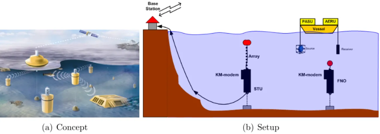
The FP7 Underwater Acoustic Network (UAN) project’s objective is to conceive, develop and test at sea an innovative wireless network integrating submerged, terrestrial and aerial sensors for the protection of off-shore and coastline critical infrastructures. In particular UAN focuses on a security oriented underwater wireless network infrastructure, realized by hydroacoustic communication.The following figure 1.1(a) presents a concept figure of the UAN network.

(a) Concept (b) Setup

Figure 1.1: UAN project: conceptual view (a) and UAN system components (b).

Figure 1.1(b) presents the UAN components which include: the Subsurface Telemetry Unit (STU), a power and communications cable to shore and a base station (BS); the dedicated modem for testing purposes, composed of the Portable Acoustic Source Unit (PASU) and the Acoustic Emission and Receive Unit (AERU) and the autonomous Fixed Underwater Nodes (FNO).

The objective of this simulation was to define the requirements for the mooring of the subsurface telemetry unit with special regard to the stability and safety of the acoustic release and array, these are described in the following sections.

Chapter 2

Description

Nine different buoy configurations were developed to compare values critical to the safety of the acoustic release - an essential element for a successful recovery of the telemetry unit. Only the height of the acoustic release was changed, adding additional weight to the buoy because of the cable connecting the telemetry unit to the on-shore base station. To compare the dynamic behavior of the mooring all buoy configurations were simulated in six different currents from 0.1m/s to 0.5m/s. For further details see section 5.1. The dynamic behaviour of the mooring was carried out with the Mooring Design & Dynamics (MD&D) Matlab package from Richard K. Dewey “Centre for Earth and Ocean Research” (University of Victoria, BC, Canada) 1. For simulation proposes all the elements in the mooring were approximated by cylinders or spheres.

1_{URL: http://canuck.seos.univ.ca/rkd/mooring/mdd/mdd.html}

Chapter 3

Buoy design

Sections 4.9 and 4.8 show the selected mooring equipment. The database used in all moor-ing configurations is called db v2moormoor-ings.mat. It should be renamed to mdcodes.mat and loaded into the MD&D program as a first step before simulation or building.

Naming conventions: The different buoy configurations were named by the length of the used bottom steel cable and the height of the STU above ground. This means a <length> of 10m results in a steel cable length of 2m, a <length> of 11m in a cable length of 3m and so on.

Chapter 4

Equipment Modeling

4.1

Cables

Cables are made of 3/8 in. Kevlar, with the lengths specified by the modified draft of the mooring.

The cable connecting the anchor and the releaser is made of thicker steel (3/8 wire rope) and varies in each mooring design from 2m to 10m in steps of 1m.

A cable connecting the STU to the base station was also clamped on to the bottom of the STU, adding additional weight. This weight depends on the length of the anchor-releaser cable (which varies from 15.71 m to 28.27 m in steps of 1.57 m). Its weight of 145 kg/km and the diameter of 1.93cm were taken from the Hydrocable manual, its drag coefficient assumed to be the same as with Kevlar cables (1.3). [4]

4.2

Subsurface float

The dimensions SUBS B3 subsurface float were estimated as a sphere of 39cm vertical height and 37.5cm diameter. It’s buoyancy of 52kg and its drag coefficient of 0.6 were taken from http://www.openseas.com/s_b3pict.htm.

4.3

Array

The specifications of the array were taken from the project plan (p. 43), with the example of the buoyancy. This value was taken from the SiPLAB report 03/06 as a negative buoyancy of 12 kg. The array is attached as a clamp-on device to the top Kevlar cable.

6 CHAPTER 4. EQUIPMENT MODELING

4.4

Sphere

A Vitrovex sphere 17”/14 with a depth rating of 6700m was used. The technical specifi-cations were taken from http://www.nautilus-gmbh.com/english/vitrovex.html and the drag coefficient of 0.95 was taken from the project plan (p. 43).

4.5

STU & modem

The STU and the surrounding cage was estimated as a cylinder with a height of 120cm and a diameter of 7cm. Its drag coefficient of 1.3 was taken from the project plan. [5]

The buoyancy was calculated by its upward force of 18.827 kg (volume of cylinder multiplied with density of sea water, 1025 kg/m3_{) minus the actual weight of the STU}

and the surrounding cage (36.170 kg + 9.453 kg). This results in a negative buoyancy of 26.795 kg. [1]

The specifications of the modem were considered equal to a single Model 111 acoustic release (84cm length, 10.2cm diameter, drag coefficient 1.3). The modem is attached as a clamp-on device to the top of the STU.

4.6

Acoustic release

The negative buoyancy of the acoustic release was taken from the Model 111 manual (1kg) as well as the dimensions (84cm length, 14.4cm diameter). The drag coefficient of 1.3 was taken from the project plan (p. 43). [3]

4.7

Anchor

The anchor was designed as a 1 Large St/C Tir with a negative buoyancy of 150kg. Its shape was approached as a steel cylinder of 15cm height and 50cm diameter. Its drag coefficient (taken from the MD&D program) was 1.3.

4.8. MOORING ELEMENTS AND SIMULATION CHARATERISTICS 7

4.8

Mooring elements and simulation charateristics

Mooring elements Simulation element # element Shape Buoy-ancy [kg] Dimensions Drag coeffi-cient Tension Mate-rial height or width [cm] diameter [cm] SUBS B3 subsurface buoy 1 SUBS B3 Sphere 52 39 37.5 0.6 Steel 36m Kevlar rope 2 3/8 Kevlar Cylinder -0.02 3600 0.9 1.3 Kevlar Array Clamp-on device #1: Hydrophone Array Cylinder -12 3400 4 1.3 Kevlar Sphere 3 Vitrovex Sphere Sphere 26 43.2 43.2 0.95 Steel 0.5m Kevlar rope 4 3/8 Kevlar Cylinder -0.02 500 0.9 1.3 Kevlar

STU & cage 5

STU/cage

Cylinder -26.8 120 7 1.3

Alumini-um STU Modem Clamp-on

de-vice #2: STU Modem Cylinder -0.5 84 10.2 1.3 Alumini-um 6m Kevlar rope 6 3/8 Kevlar Cylinder -0.02 6000 0.9 1.3 Kevlar

Hydrocable Clamp-on de-vice #3: Hydrocable Cylinder -2.278 to - 4.1 1571 to 2827 1.9 1.3 Kevlar Releaser 7 Model111 AR Cylinder -1 84 14.4 1.3 Alumini-um Steel rope 8 3/8 wire rope Cylinder -0.33 2000 to 10000 0.9 1.3 Steel Anchor 9 1 Large St/C Tir Cylinder -150 15 50 1.3 Steel

8 CHAPTER 4. EQUIPMENT MODELING

4.9

Draft

Figure 4.1: Draft of used mooring elements.

Chapter 5

Dynamic behaviour of the mooring

5.1

Environmental conditions

The present mooring is expected to be done in the same location as MREA’07. During MREA’07 the maximum currents measured by a waverider buoy were: from bottom to top smaller than 0.01m/s, in north direction smaller than 0.2m/s and in east direction smaller than 0.07m/s.

For simulation proposes six different currents were used to compare the resulting angles of the buoy elements. This was done by using vectors in x (east) and y (north) directions with a resulting vector in xy-direction of 0.5, 0.4, 0.3, 0.25, 0.2 and 0.1 m/s. The velocities were associated to depths of 100m, 60m and 30m (with the velocity independent to depth). Sea ground speed was 0 m/s. No vertical currents were used. [2]

As the considered buoy will be situated more than 50m below sea level, no surface winds were simulated. Standard densities given by the MD&D software were used (1024-1026 kg/m3_).

See files EnvCond <current>mps.mat for all used environmental conditions.

5.2

Results

See files SimulatedMooring Graph res<current>.pdf, Positions+Angles res<current>.pdf and Additional AnchorDetails.pdf for results of each mooring design. See MooringElements.pdf and STU mooring <length>.mat for the used mooring configuration.

10 CHAPTER 5. DYNAMIC BEHAVIOUR OF THE MOORING

5.2.1

Angles

For each mooring configuration the angles of the bottom steel cable (connecting the anchor and the acoustic releaser) and of the acoustic array (measured via the top Kevlar cable) were taken into special consideration because of their importance to the whole buoy.

Different steel cable lengths and currents were used and a spreadsheet comparing the results was provided. See Angles.ods for further details and Angles.pdf for a graphical overview.

Figure 5.1: Mooring Angle relative to water current

5.2. RESULTS 11

Figure 5.2: Mooring Angle relative to water current

12 CHAPTER 5. DYNAMIC BEHAVIOUR OF THE MOORING

5.2.2

Height above ground

For each mooring configuration the height of the acoustic release above sea ground was taken into special consideration because of its importance to the recovery of the buoy.

For each buoy configuration a worst case current of 0.5m/s was assumed and the re-sulting heights of the acoustic release were compared. See HaG.ods for further details and HaG.pdf for a graphical overview. As shown there is an effective loss of approx. 20cm of the individual steel cable length because of currents.

Figure 5.3: Mooring Height Above ground relative to water current

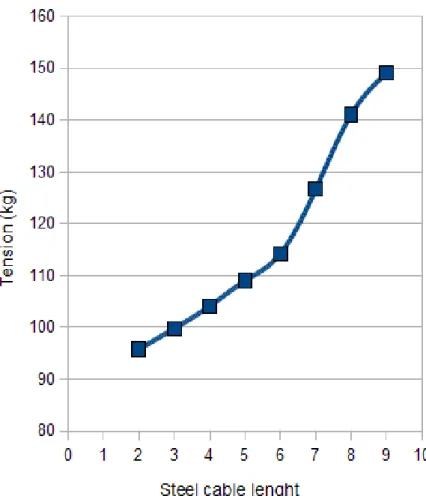
5.2.3

Tension on Anchor

Another value of specific interest to the safety of the mooring is a sufficient anchor. For each buoy configuration a possible worst case current of 0.5m/s was assumed and the resulting total tensions on the anchor were compared. The results were also broken down to all configurations and currents from 0.1m/s to 0.5m/s. See Tension Anchor.ods for further details and Tension Anchor.pdf for a graphical overview. Due to limitations of the MD&D program no tensions higher than the weight of the anchor could be sufficiently simulated.

An additional weight to the planned anchor (150kg) is strongly recommended.

5.2. RESULTS 13

Figure 5.4: Mooring Tension on Anchor

Chapter 6

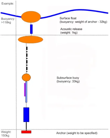
Deployment Float

A surface float is needed for deployment of the subsurface buoy. Its buoyancy should be sufficient to keep the whole buoy including the anchor at the sea surface to make a safe deployment possible. The subsurface floats (SUBS B3 and the Vitrovex sphere) have a combined buoyancy of 78kg, the equipment and cables have a combined weight of approx. 46kg plus the weight of the chosen anchor. This results in a minimum buoyancy of the surface float of -32kg plus the weight of the anchor. For example, if the anchor has a weight of 150kg, the minimum surface buoyancy is 118kg. Appropriate safety factors should be considered.

Figure 6.1: Deployment and Mooring Setup

Chapter 7

Conclusions

During the simulations various situations were modeled and the results presented in angle relative to sea floor, the resulting height above sea floor and tensions on the anchor. The range of water column current was simulated between 0.1 m/s and 0.5 m/s, standard values obtained during a previous sea trial for the region of operation had a maximum of 0.2 m/s. The results show that for the value of 0.2 m/s and the modelized equipment the mooring had a 20◦ declination from the vertical position which is an acceptable value, the simulations also show that an increase in the length of the bottom mooring cable results in an include in declination probably because of the weight of the steel cable. From the simulation of the tension the results presented a value of 150 kg in the worst case. It is so suggested to place at least a 200kg weight as the anchor as the remainder of the equipment can not be varied for the current setup.

Appendix A

STU/cage weight calculations

The buoyancy of the STU and the cage was calculated as described below: STU: V = [(16cm)2∗ π ∗ 60cm] − [(15cm)2_{∗ π ∗ 60cm]} + 6 ∗ (1.3cm ∗ 1.6cm ∗ 60cm) + 2 ∗ [(15.156cm)2∗ π ∗ 4.7cm] + 2 ∗ (3cm ∗ 3cm ∗ 1.5cm) = 0.013396153181376m3 m = 0.013396153181376m3∗ 2700kg/m3 = 36.1696135897152kg Cage: V = 7 ∗ ([(24cm)2∗ π ∗ 0.6cm] − [(22.8cm)2∗ π ∗ 0.6cm]) + [(21.6cm)2∗ π ∗ 0.6cm] − [(20.4cm)2 _{∗ π ∗ 0.6cm]} + 3 ∗ (1.6cm ∗ 120cm ∗ 0.6cm) = 0.00118161550423208706m3 m = 0.00118161550423208706m3∗ 8000kg/m3 = 9.45292403385669648kg Water cylinder: V = π ∗ (9.3cm)2∗ 67.6cm = 0.01836802516597m m = V ∗ 1025kg/m3 = 18.82722579511925kg 16

17

Buoyancy:

m = 18.82722579511925kg − 36.1696135897152kg − 9.45292403385669648kg = −26.79531182845264648kg

Appendix B

Current vector calculations

|~x + ~y| =px2_{+ y}2

~x = ~y (identical currents in x and y direction) r =√2 ∗ x2 _{(value of resulting current)}

x =pr2_{/2 (current in x or y direction)} r = 0.5 ⇒ x ≈ 0.35 r = 0.4 ⇒ x ≈ 0.28 r = 0.3 ⇒ x ≈ 0.21 r = 0.25 ⇒ x ≈ 0.18 r = 0.2 ⇒ x ≈ 0.14 r = 0.1 ⇒ x ≈ 0.07 18

Appendix C

AR diameter calculations

V1 = π ∗ a2∗ h (a = used mean diameter)

V2 = 2 ∗ (π ∗ r2∗ h) (Volume of both ARs)

V1 = V2 ⇒ a = r ∗ √ 2 (solve equation) r = 10.2cm a = 14.42497833620557cm 19

Appendix D

Hydrocable length calculations

The length was considered as the quarter of the outline of an circle with a radius varying from 10m to 18m in steps of 1m.

l = 0.25 ∗ (2 ∗ π ∗ r) (l = cable length, r = distance to ground) b = l ∗ 0.145kg/m (b = neg. buoyancy) r = 10m ⇒ l = 15.7079632679490m ⇒ b = 2.277654673852605kg r = 11m ⇒ l = 17.2787595947439m ⇒ b = 2.5054201412378655kg r = 12m ⇒ l = 18.8495559215388m ⇒ b = 2.733185608623126kg r = 13m ⇒ l = 20.4203522483337m ⇒ b = 2.9609510760083865kg r = 14m ⇒ l = 21.9911485751286m ⇒ b = 3.188716543393647kg r = 15m ⇒ l = 23.5619449019235m ⇒ b = 3.4164820107789075kg r = 16m ⇒ l = 25.1327412287184m ⇒ b = 3.644247478164168kg r = 17m ⇒ l = 26.7035375555133m ⇒ b = 3.8720129455494285kg r = 18m ⇒ l = 28.2743338823082m ⇒ b = 4.099778412934689kg 20

Appendix E

STU height calculations

The STU was approximated as a cylinder with the volume of the STU alone (see STU drawings.pdf, p. 12), but with the height of the full cage. The resulting diameter was then calculated:

V1 = r12∗ π ∗ h = (18.6cm/2)2∗ π ∗ 68cm (STU volume)

V2 = r22∗ π ∗ h = r22∗ π ∗ 120cm (new cylinder)

V1 = V2 ⇒ r2 = 7.00077819824219cm