An Error Bound for Low Order Approximation of Dynamical Systems Subjected to Initial Conditions

doi: 10.5540/tema.2018.019.02.0197

An Error Bound for Low Order Approximation of

Dynamical Systems Subjected to Initial Conditions

G.P.R. MACIEL*and R.S. BARBOSA

Received on July 31, 2017 / Accepted on November 21, 2017

ABSTRACT. In recent years, a great effort has been taken focused on the development of reduced order modeling techniques of dynamical systems. This necessity is pushed by the requirement for efficient numer-ical techniques for simulations of dynamnumer-ical systems arising from structural dynamics, controller design, circuit simulation, fluid dynamics and micro electromechanical systems.

We introduce a method to calculate the minimum upperL_{2error bound of a linear time invariant reduced}

or-der model consior-dering any possible unitary initial conditions (IC). As a consequence, the proposed method calculates the unitary IC vector which leads to the maximumL_{2norm of the error. Based on this error}

bound, it is discussed the capacity of a reduced order system to approximate the free transient response in the worst case scenario.

Keywords: Model reduction, dynamical systems, observability grammian, initial condition, error bound.

1 INTRODUCTION

Even with the advances in computer technology, which considerably increased computational processing capacity and storage in the last decades, the demand for increasing the complexity of dynamical systems is still a major concern. To handle this problem, a great effort is being taken towards the development of methods to calculate reduced order models (ROM) that repro-duce the main dynamic characteristics of a high order model (HOM) with a rerepro-duced demand on computational processing capacity, memory and computing time [1, 2, 3, 6, 7, 11, 21].

The determination of error bounds associated with reduced models plays an important role in the development of such Model Order Reduction (MOR) methods. It allows to predict the maximum (or minimum) error associated to the lower order approximation without the need of performing excessively time-demanding simulations. Furthermore, the a priori knowledge of error bounds allows the comparison of different MOR methods and for consequence the selection of the most suitable method to each application based on a prescribed threshold for the ROM error.

*Corresponding author: Gabriel Pedro Ramos Maciel – E-mail: ga.pe.01@gmail.com

In an early work, a method is proposed for MOR which guarantees anL_{2-optimal error bound} for the impulse response of Multi-Input-Multi-Output (MIMO) dynamical systems [26].

MOR methods based on modal truncation have advantages compared to other methods due to the physical interpretation of the retained and eliminated eigenmodes, moreover it preserves the original poles of the retained eigenmodes. In the literature one can find proposals of different H_{∞-norm error bounds for different modal MOR methods [6, 25, 14].}

Another approach to the error bound calculation of ROM is the approximation of theH_2and H_{∞norms for modal MOR methods, found in [12]. This work shows a selection criteria for the} eliminated eigenmodes based on the a priori aproximation of the error norms.

A selection criteria was proposed for the truncation of eigenmodes which minimizes theH₂ -norm of the error associated to modal truncation method [23].

Methods to calculate theH_2andH_{∞error norms for ROM in the balanced realization base are} presented in [13] and [1].

A method to compute the suboptimalH_{∞-norm error bound shows a suboptimal approach to the} task of minimizing theH_{∞-norm of the ROM error [19] and have advantages over other Hankel} optimal MOR techniques such as better lower error bounds.

A frequency weighted technique for balanced MOR was proposed by Imran et al. [16], which also introduces a frequency weightedH_{∞-norm of the ROM error.}

In a recent work, an error bound for the MOR of delay linear and nonlinear systems is proposed [24]. This method also preserves the stability in the reduced order model.

The IC problem for nonlinear reduced order dynamical systems was obtained using the Center Manifolds Method [8]. A method is proposed to calculate the initial conditions of the ROM based on de IC of the HOM. Nevertheless, error bounds of the ROM response are not discussed in this work.

Due to the importance of determining error bounds for a ROM, this work introduces a method to calculate the minimumL_{2-error upper bound for the free transient IC response of a truncated} ROM. This upper bound measures the capability of the reduced system to reproduce the free transient IC response of the HOM considering all possible unitary initial conditions, which rep-resents the worst case scenario for this problem. The error bound is first presented regardless the basis onto which the model is projected and than it is showed a specific case for the MOR based on modal coordinates.

2 PROBLEM STATEMENT

Consider a linear, time-invariant, asymptotically stable, continuous-time, dynamical system

[A,B,C,D]in its minimal realization, with the following state space representation:

Wherex(t)∈Rn,u(t)∈Rnu,y(t)∈Rnyare respectively the state vector, input vector and output vector. Hence,nis the order (or state space dimension) of the system andA∈Rnxn,B∈Rnxnu,

C∈Rnyxn_andD∈Rnyxnu_.

The initial state of the system in eq 2.1 isx(0) =x0_{and the upperscore} 0_{in state vectors are}

herein representing the initial sate (or the IC) of the corresponding system.

This system is herein called a high order dynamical system, or high order model (HOM) of order n. It is intended to calculate a ROM[Ar,Br,Cr,Dr]of ordernr≤nwhich is capable to reproduce

the overall dynamic behavior of the HOM.

˙xr(t) =Arxr(t) +Bru(t) yr(t) =Crxr(t) +Dru(t) (2.2)

Wherexr∈Rnr,Ar∈Rnrxnr,B∈Rnrxnu,C∈Rnyxnr andD∈Rnyxnu and the initial state of this system isxr(0) =x0

r.

Without loss of generality, the HOM can be partitioned onto the most dominant and less dominant Degree of freedom (DOF)x1∈Rnr _andx2∈Rn−nr _{respectively:}

     ˙x1 ˙x2 y      =   

A11 A12 B1 A21 A22 B2 C1 C2 D

        x1 x2 u      (2.3)

It is assumed that the most dominant and less dominant DOF are selected according to an arbi-trary selection criterion. A detailed review and descritption of the less dominant DOF selection criteria can be found at [1, 5, 18].

It is considered that the ROM is obtained by the truncation of the less dominant DOF vectorx2.

Considering this,Ar=A11,Br=B1,Cr=C1andDr=D.

The system which describes the dynamics of the errore(t) =y(t)−yr(t)between the HOM and ROM is[Ae,Be,Ce,De], which is:

         ˙x1 ˙x2 ˙xr e          =     

A11 A12 0 B1 A21 A22 0 B2 0 0 A11 B1 C1 C2 −C1 0

              x1 x2 xr u          (2.4)

Where ˆx={x1;x2;xr}is the state vector for the system in eq. 2.4 andAe∈R(n+nr)x(n+nr)_{. The} respective IC vector is ˆx0={x0

1;x02;x0r}.

The error function is herein defined as theL_{2norm of the error vectore(}t), represented by the notationkekL₂. Where

kek2L₂=

Z ∞

0 e

T_(τ)e(τ)dτ

(2.5)

is the norm in the function spaceLny

2 of Lebesgue integrable functionse:[0,∞)→R

Considering this, the intention of the following section is to determine the minimumkekL₂ for the free transient response of the ROM subjected to any possible initial conditions.

ε_0=max{kekL

2 | ˆx 0_∈

Rn+nr;u(t) =0} (2.6)

3 A MINIMUML_{2-ERROR UPPER BOUND FOR THE IC PROBLEM}

The observability grammianQof the system in eq. 2.4 can be calculated using the following Lyapunov equation:

AT_eQ+QAe+CTeCe=0 (3.1)

The observability grammian Q is symmetric positive semi-definite for asymptotically stable systems and it can be partitioned as

Q=



 

Q11 Q12 Q13 QT

12 Q22 Q23 QT₁₃ QT₂₃ Q33





 (3.2)

WhereQ∈Rn+nrxn+nr,Q11∈Rnrxnr andQ33∈Rnrxnr.

Using the partitioned form in eq. 2.4 and substituting eq. 3.2 in eq. 3.1, the solution for the observability grammian can be decoupled into 3 lower order Lyapunov equations:

AT

"

Q11 Q12 QT

12 Q22

#

+

"

Q11 Q12 QT

12 Q22

#

A+CTC=0 (3.3)

AT₁₁h QT₁₃ QT₂₃ i+h QT₁₃ QT₂₃ iA−CT₁C=0 (3.4)

AT11Q33+Q33A11+CT1C1=0 (3.5)

One can observe that the calculated blocks{{Q11,Q12};{Q21,Q22}}in eq. 3.3 corresponds to

the observability grammian of the HOM. Analogously, the blockQ33calculated in eq. 3.5 is the observability grammian of the ROM.

Given a non trivial IC to the HOMx06=0

x0={x0

1;x02} (3.6)

and the IC vector of the system in eq 2.4 isˆx0={x0

1;x02;x0r}.

Considering that the ROM is obtained by the truncation of the least significant DOF of the HOM, the IC vector of the ROM is consequently obtained by the truncation of the IC vector of the HOM:

x0_r =x0₁ (3.7)

From eq. 3.7, the IC vector of the system in eq 2.4 isˆx0={x0

1;x02;x01}.

It is considered that the error functionkekL₂for the IC problem is:

kek2L₂=

Z ∞

0 e

T_{(τ)e(τ)dτ= (ˆx}0₎T_Qˆx0

Substituting eq. 3.2 into eq. 3.8 and performing simbolic manipulation, the error funcionkekL₂

can be calculated as

kek2

L₂= (x0)TQex0= (x0)T

"

Q11+Q13+QT

13+Q33 Q12+QT23 QT₁₂+Q23 Q22

#

x0 (3.9)

From eq 3.9, the eq. 2.6 can be rewriten and the minimum upper bound ε_{0 of kek}L₂ for all

possible unitary initial conditions is:

ε_0=max{kekL

2 | x0∈R n

;kx0k=1;u(t) =0} (3.10)

Considering that the solution of eq. 3.1 is positive semidefinite [17] with real nonnegative eigenvalues, the solution of the eq. 3.10 is:

ε2

0=max i abs(

λ_{i(Qe)) =abs(}λ_{max(Qe)) (3.11)}

Whereabs(λ_{i(Qe))is the absolute value of the i-th eigenvalue ofQeand}λ_{max(Qe)is the largest}

eigenvalue ofQe.

It is important to notice that the eigenvector associated toλ_{max(Qe)is the IC that maximizes the}

errorkekL₂. In other words, it is the scenario which the ROM provides the highestL_{2-error of} the free transient response to the IC problem.

3.1 Error bound due to initial conditions on modal coordinates

Modal methods intends to catch the behaviour of the dominant eigenmodes of the HOM into the ROM. In order to do that, the state-space is projected on the subspace spanned by a set of eigenvetors which are considered most dominant [10]. Different selection criteria to elect the most dominant eigenvectors can be found in the literature [21, 25, 12, 15, 22].

Before the truncation of the less dominant states, the HOM can be projected onto an orthonormal modal base [20]. Let us assume that the realization in eq. 2.1 is diagonalizable such that

˙

w(t) =Aw(˜ t) +Bu(˜ t) y(t) =Cw(˜ t) +Du(˜ t) (3.12)

Where[_A˜,B˜,C˜,D]˜ is the HOM projected onto the modal basis and:

x(t) =Φw(t) ˜

A=Φ−1AΦ=diag(λ₁,λ2, . . . ,λn)

˜

B=Φ−1B ˜

C=CΦ

˜ D=D

(3.13)

Thus, the system in the modal form can be partitioned as in eq. 2.3 withw(t) ={w1(t);w2(t)}. Wherew1(t)andw2(t)are the most cominant and less dominant DOF respectively.

     ˙ w1 ˙ w2 y      =    ˜

A11 0 B˜1 0 A22˜ B2˜

˜

C1 C2˜ D˜

        w1 w2 u      (3.14)

The reduction by truncation is applied in eq. 3.14 and the error system[Ae˜ ,Be˜ ,Ce˜ ,De]˜ is

           ˙ w1 ˙ w2 ˙ wr ˜e            =       ˜

A11 0 0 B1˜ 0 A22˜ 0 B2˜ 0 0 A˜11 B˜1 ˜

C1 C2˜ −C1˜ 0

               w1 w2 wr u          (3.15)

Withwˆ ={w1;w2;wr}is the state vector of eq. 3.15 and˜e(t)is the error of the ROM model in the modal basis.

The eq. 3.15 can be simplified to its minimal realization, showed in 3.16.

( ˙ w2 ˜e ) = " _˜

A22 B˜2 ˜ C2 0 # ( w2 u ) (3.16)

The observability gramianQe˜ for the modal form can be calculated from eq. 3.16.

˜

AT₂₂Qe˜ +Qe˜ A22˜ +C˜T₂C2˜ =0 (3.17)

The method to calculate the observability grammian of the error system using eq. 3.17 requires considerable less computational processing capacity and memory than the method to calculate the grammian using the high order Lyapunov equation to the system in eq. 3.15. The solution of Lyapunov equations involving lower order matrices, as described in this method, is a great advantage considering the high computational effort and memory involved in the solution of this type of problem [4, 9]

The normk˜ekL₂ for a given ICw0

2=w2(0)for eq. 3.16 is

k˜ek2L₂= (w02) T_˜

Qew02 (3.18)

Consequently, the minimumL_{2-error upper bound ˜}ε_{0 of the ROM in the modal base, for any}

given ICw(0)(applied at the HOM described in eq. 3.15) is

˜

ε2 0=max

i abs

λ_i(Qe)˜

=abs λ_max(Qe)˜

(3.19)

4 EXAMPLE

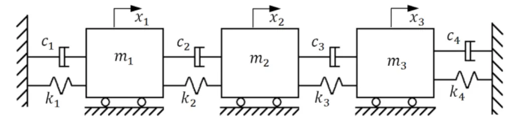
The parameter values are: m1=1kg, m2=0.1kg, m3=1kg, k1=1N/mm, k2=0.1N/mm,

k3=0.5N/mm, k4=2N/mm, c1=0.2N/(mm/s), c2=0.1N/(mm/s), c3=0.1N/(mm/s), c4=

0.5N/(mm/s).

Figure 1: Mass-spring-damper system with 3 bodies.

The state space vetor isx={x1,x˙1,x2,x˙2,x3,x˙3}and HOM can be written as

                       ˙ x1 ¨ x1 ˙ x2 ¨ x2 ˙ x3 ¨ x3 y                        =            

0 1 0 0 0 0 0

−k1+k2 m1 −

c1+c2 m1

k2 m1

c2

m1 0 0

1 m1

0 0 0 1 0 0 0

k2 m2

c2 m2 −

k2+k3 m2 −

c2+c3 m2

k3 m2

c3 m2 0

0 0 0 0 0 1 0

0 0 k3

m3

c3 m3 −

k3+k4 m3 −

c3+c4 m3 0

0 0 1 0 0 0 0

                                   x1 ˙ x1 x2 ˙ x2 x3 ˙ x3 u                        (4.1)

Two reduced models, herein called RO and RM, were calculated by applying the truncation of 2 states in the original and modal basis respectively. Equation 4.2 shows the RO model which state vector isxRO={x˙RO1;xRO1; ˙xRO2;xRO1}

             ˙ xRO1 ¨ xRO1 ˙ xRO2 ¨ xRO2 yRO              =       

0 1.0 0 0 0

−1.1 −0.3 0.1 0.1 1.0

0 0 0 1.0 0

1.0 1.0 −6 −3 0

0 0 1.0 0 0

                    xRO1 ˙ xRO1 xRO2 ˙ xRO2 u              (4.2)

Equation 4.3 shows the RM model, obtained by truncating the HOM in the modal basis, which state vector iswRM={w˙RM1;wRM1; ˙wRM2;wRM1}

             ˙ wRM1 ¨ wRM1 ˙ wRM2 ¨ wRM2 yRM              =       

−0.1248 1.0303 0 0 1.4843

−1.0303 −0.1248 0 0 −0.1391

0 0 −0.2962 1.3576 −0.3413

0 0 −1.3576 −0.2962 0.1140

0.0696 −0.2477 −0.0934 −0.4280 0

5 RESULTS

Although it is not necessary for the determination of the error bounds, complete and reduced models were simulated subjected to IC in order to demonstrate the dynamic behavior of the error in the worst case scenario.

Figure 2 shows the response of the complete and reduced RO models subjected to the ICxλ_max(0) andxROλ_max(0) =respectively.

xλ_max(0) ={ −0.0136; 0.0895 −0.0978 −0.0157 −0.0832 −0.4291 }

xROλ_max(0) ={ −0.0136 0.0895 −0.0978 −0.0157 }

The vectorxλ_max(0)is the eigenvector associated to the eigenvalueλmax(Qe)specified in eq. 3.11, withkxλ_max(0)k=1. Consequently,xROλ_max(0)is the IC vector for the truncated reduced model.

Figure 2: Dynamic simulation of complete and reduced RO system (original basis).

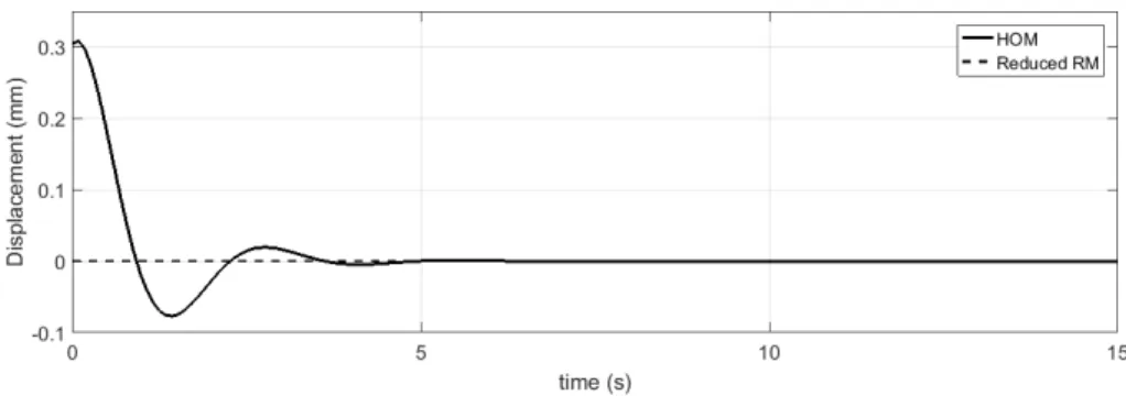
Figure 3 shows the response of the complete and reduced RM models (both in the modal basis) subjected to the ICwλ_max(0)andwRMλ_max(0) =respectively.

wλ_max(0) ={ 0 0 0 0 −0.1611 0.9869 }

wRMλ_max(0) ={ 0 0 0 0 }

The vectorwλ_max(0)is the eigenvector associated to the eigenvalueλmax(Q˜e)specified in eq. 3.19, withkwλ_max(0)k=1. Consequently,w_RMλ_max(0)is the IC vector for the truncated reduced model.

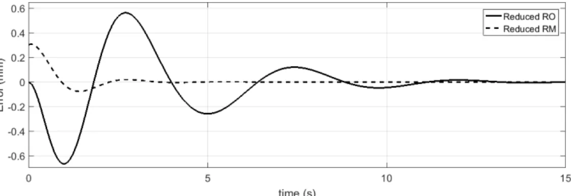
Figure 4 shows the error of the reduced RO and RM systems subjected to the above mentioned initial conditions.

Using eq. 3.11 and eq. 3.19, the error boundsε_{0and ˜}ε_{0, for the reduced models RO and RM}

Figure 3: Dynamic simulation of complete and reduced RM system (modal basis).

Figure 4: Error of the reduced order systems.

Table 1: Error bounds andL_{2error norms calculated from simulations.}

Reduced model error bound(1) L_{2-norm of the error}(2)

RO (original basis) ε_{0=0.8885 0.8885}

RM (modal basis) ε˜_{0=0.2119 0.2119}

(1)_{calculated using eq. 3.11 and eq. 3.19} (2)_{calculated using eq. 2.5}

6 CONCLUSIONS

Later, the special case for MOR by modal truncation was presented and discussed. The pro-posed method also have the advantage of a considerable less computational processing capacity and memory to the calculate the observability gramian of the error system. This leads to a con-siderable time, hardware and memory savings when the method is applied to extremely large systems.

The advantages of using the presented method is that the minimum upper bound of theL_2error can be calculated without the necessity to perform the free transient analysis of the error.

According to the numerical results, the error bound of the reduced model by modal truncation (RM) is smaller than the truncation in the original basis (RO), such a result indicates that the reduction by modal truncation is a better approximation than the truncation in the original basis for the free transient response approximation.

RESUMO. Nos ´ultimos anos, um grande esforc¸o tem sido realizado para se obter modelos de sistemas dinˆamicos de ordem reduzida. Esta necessidade ´e impulsionada pela demanda por t´ecnicas mais eficientes para simular sistemas dinˆamicos em ´areas como dinˆamica de estruturas, projeto de controladores, circuitos eletrˆonicos, dinˆamica de fluidos e sistemas microeletromecˆanicos.

Os autores prop˜oem um m´etodo para calcular o limite superior m´ınimo da normaL₂ do erro de um sistema linear invariante no tempo e de ordem reduzida, considerando todas as poss´ıveis combinac¸˜oes de condic¸˜oes iniciais unit´arias. Consequentemente, o m´etodo pro-posto calcula o vetor unit´ario de condic¸˜oes iniciais que maximiza a norma L₂ do erro do sistema reduzido. Baseado neste limite de erro, avalia-se a capacidade que um sistema dinˆamico de ordem reduzida possui para aproximar a resposta transit´oria frente a condic¸˜oes iniciais.

Palavras-chave: Reduc¸˜ao da ordem de modelos, sistemas dinˆamicos, gramiano de observabilidade, condic¸˜oes iniciais, limite de erro.

REFERENCES

[1] A.C. Antoulas. “Approximation of large-scale dynamical systems”, volume 6. Siam (2005). doi:10. 1137/1.9780898718713.

[2] A.C. Antoulas, D.C. Sorensen & S. Gugercin. A survey of model reduction methods for large-scale systems.Contemporary mathematics,280(2001), 193–220.

[3] Z. Bai. Krylov subspace techniques for reduced-order modeling of large-scale dynamical systems.

Applied numerical mathematics,43(1-2) (2002), 9–44.

[4] U. Baur & P. Benner. Factorized solution of Lyapunov equations based on hierarchical matrix arithmetic.Computing,78(3) (2006), 211–234.

[6] P. Benner. “Numerical linear algebra for model reduction in control and simulation”, volume 29. Wiley Online Library (2006), pp. 275–296.

[7] P. Benner, V. Mehrmann & D.C. Sorensen. “Dimension reduction of large-scale systems”, volume 45. Springer (2005).

[8] S.M. Cox & A. Roberts. Initial conditions for models of dynamical systems.Physica D: Nonlinear Phenomena,85(1) (1995), 126–141.

[9] B.N. Datta. “Numerical methods for linear control systems: design and analysis”, volume 1. Academic Press (2004).

[10] E. Davison. A method for simplifying linear dynamic systems. IEEE Transactions on automatic control,11(1) (1966), 93–101.

[11] R.W. Freund. Model reduction methods based on Krylov subspaces.Acta Numerica,12(2003), 267– 319.

[12] W.K. Gawronski. “Dynamics and control of structures: A modal approach”. Springer Science & Business Media (2004).

[13] K. Glover. All optimal Hankel-norm approximations of linear multivariable systems and theirL_∞ -error bounds.International journal of control,39(6) (1984), 1115–1193.

[14] M. Green & D.J. Limebeer. “Linear robust control”. Courier Corporation (2012).

[15] C. Gregory. Reduction of large flexible spacecraft models using internal balancing theory.Journal of Guidance, Control, and Dynamics,7(6) (1984), 725–732.

[16] M. Imran, A. Ghafoor & V. Sreeram. A frequency weighted model order reduction technique and error bounds.Automatica,50(12) (2014), 3304–3309. doi:10.1016/j.automatica.2014.10.062.

[17] P. Lancaster & M. Tismenetsky. “The theory of matrices: with applications”. Elsevier (1985).

[18] G.P.R. Maciel. “M´etodos de reduc¸˜ao de graus de liberdade em sistemas dinˆamicos lineares”. Master’s thesis, Escola polit´ecnica da Universidade de S˜ao Paulo (2015).

[19] A. Megretski. H-infinity model reduction with guaranteed suboptimality bound. In “American Control Conference, 2006”. IEEE (2006), pp. 6–6. doi:10.1109/ACC.2006.1655397.

[20] L. Meirovitch. “Computational methods in structural dynamics”, volume 5. Sijthoff & Noordhoff International Pub (1980).

[21] G. Obinata & B.D. Anderson. “Model reduction for control system design”. Springer Science & Business Media (2012).

[22] L. Pernebo & L. Silverman. Model reduction via balanced state space representations. IEEE Transactions on Automatic Control,27(2) (1982), 382–387.

[24] N. van de Wouw, W. Michiels & B. Besselink. Model reduction for delay differential equations with guaranteed stability and error bound.Automatica,55(2015), 132–139. doi:10.1016/j.automatica. 2015.02.031.

[25] A. Varga. On modal techniques for model reduction. Technical report, Technical Report TR R136-93, Institute of Robotics and System Dynamics, DLR Oberpfaffenhofen, PO Box 1116, D-82230 Wessling, Germany (1993).