A simulation analysis of the impact of forest fire suppression policies on rekindles

Faculdade de Engenharia da Universidade do Porto

A simulation analysis of the impact of forest fire

suppression policies on rekindles

David Pereira da Silva

Dissertation in the scope of

Mestrado Integrado em Engenharia Electrotécnica e de Computadores

Major Automação

Supervisor: João Claro

Co-supervisor: Abílio Pereira Pacheco

29/07/2016

Abstract

During the season with more forest fires in Portugal (Charlie, from July through September) it is usual to have large usage of resources, human and material, to combat forest fires, and on peak days firefighters are in a tight spot, due to the pressure to move incessantly from one fire to another. In such occasions the system may not be able to effectively meet the needs, getting out of control, in which scenarios all the help is appreciated. Fires waiting to be fought keep spreading, becoming tougher to extinguish, with an increased likelihood of reaching homes, people, animals, and destroying the landscape. Additionally, fire crews prematurely abandon mop-up operations (moving towards new battlefronts), which need time and appropriate tools to be carried out effectively. If one of these fires rekindles, it is one more to join the others, and they are generally more aggressive than primary fires (PF).

An analysis of the 2010 data for Porto, provided by the Portuguese Institute for Nature Conservation and Biodiversity (ICNF - Instituto de Conservação da Natureza e das Florestas), during these 3 months, shows that approximately 11% of the forest fires were rekindles (RKD). We used information from 2010 to be able to reuse and build upon a large volume of statistical analyses that had already been performed.

Having RKD phenomenon as a backdrop, we developed a simulation model of a suppression system, following the perspective of Pacheco, Claro, and Oliveira (2014a). Because the previously developed system was already a robust basis, we focused on including new suppression resources, such as standard (STD) crews of volunteer firemen with training, and specialized/expert (EXPRT) crews for firefighting and especially for mop-up operations, with special skills and tools to perform that operation in an effective way. The objectives of the analyses are to assess the impact that different scenarios have on RKD, and identify which would be the best solutions to implement, considering their effectiveness in terms of reducing RKD to desirable levels, different dispatch policies, and the total cost that they require.

Resumo

Durante a fase de mais incêndios florestais (Charlie) em Portugal (de Julho a Setembro) é comum haver uma grande mobilização de recursos, tanto humanos como materiais, para combater os incêndios florestais e em dias de pico os bombeiros ficam numa situação delicada devido à pressão para se moverem incessantemente de um incêndio para outro. Nessas alturas o sistema não consegue responder a todas as necessidades, levando ao descontrolo e toda a ajuda é importante. Dessa forma, os fogos em situação de espera continuam a alastrar-se, podendo atingir casas, pessoas, animais e destruir a paisagem natural. Além disso, os bombeiros têm de abandonar prematuramente a operação de rescaldo (para irem combater novos incêndios) que precisa de ferramentas apropriadas para ser executada de forma eficaz. Um incêndio que reacende é mais um a juntar-se aos outros e normalmente é mais agressivo que o seu correspondente incêndio primário.

Por análise dos dados de 2010 durante esses três meses, para o Porto, disponibilizados pelo Instituto de Conservação da Natureza e das Florestas (ICNF), concluiu-se que 11% dos incêndios florestais desse ano foram reacendimentos. Devemos dizer que utilizamos os dados de há seis anos atrás pois já tem uma forte base estatística, servindo como ponto de partida para o nosso trabalho.

Tendo os reacendimentos como pano de fundo, desenvolvemos um modelo de simulação de um sistema de supressão, numa perspetiva de seguimento de Pacheco, Claro, and Oliveira (2014a). Como o sistema anteriormente desenvolvido oferecia uma boa base estatística, focamos na inclusão de novos recursos de supressão, nomeadamente bombeiros voluntários com a possibilidade de variarmos o seu nível de formação e equipas especializadas em combater incêndios e, especialmente, em rescaldos, as quais se caracterizam por terem diferentes competências e ferramentas adequadas para realizar essa etapa de uma forma mais eficaz. O objetivo desta dissertação é analisar o impacto de diferentes cenários nos reacendimentos e, como conclusão, prever quais são as melhores soluções que se podem incorporar na realidade, tendo em consideração a sua eficácia na redução dos reacendimentos, diferentes políticas de envio e o custo total necessário para a sua execução.

Acknowledgments

The work represented here wouldn’t be possible without the extensive knowledge transmitted by my supervisor João Claro and co-supervisor Abílio Pereira Pacheco, as a result of their experience and ability to lead. Combining this with their availability and readiness to help me whenever I needed, I can only be satisfied and feel that they gave me all the conditions so that I could perform a good work, during last nine months, in the best way possible. I have also to thank the possibility of having a workplace in INESC TEC given to me, and the good environment and kindness of all the people working there.

Index

Chapter 1 ... 1

Introduction ... 1

1.1 Wildfires and rekindles ... 1

1.2 Research questions ... 2

1.3 Work context ... 2

1.4 Dissertation structure ... 3

Chapter 2 ... 4

Literature Review ... 4

2.1 Methods to deal with complexity ... 5

2.2 Methods for handling uncertainty ... 7

2.3 Forest fire management research scope ... 8

2.4 Economic models ... 10

Chapter 3 ... 12

Data and Methods ... 12

3.1 2010 forest fires ... 12

3.2 Data source ... 13

3.3 Methods used ... 13

Chapter 4 ... 16

System design ... 16

4.1 Overview of the suppression system ... 16

4.2 Features implemented ... 17

4.3 Arrivals of NF, FA and FFA ... 17

4.4 Initial Attack and Extended Attack ... 18

4.5 Rekindles generated directly from NF ... 22

4.6 Modeling the active events in the last 24 hours ... 24

4.7 Control Logic ... 25 4.8 Model validation ... 25

Chapter 5 ... 26

Results ... 26 5.1 Scenario 1 ... 27 5.2 Scenario 2 ... 30 5.3 Scenario 3 ... 31 5.4 Scenario 3, composition ... 33 5.5 Scenario 4 ... 35

Chapter 6 ... 37

Discussion ... 37

Chapter 7 ... 43

Conclusion ... 43 7.1 Limitations ... 44 7.2 Future work ... 44 References ... 45

Appendix A: Variables, expressions and other simulation elements ... 49

Appendix B: Model blocks ... 54

List of figures

Figure 1 – On the left are the highlighted values used on the interpolation on the right; as we know that 70 STD crews correspond to 464.87 RKD and 80 STD crews correspond to 366.59 RKD, we used the two points to find out the number of crews that

correspond to 435 RKD, using linear interpolation. ... 15

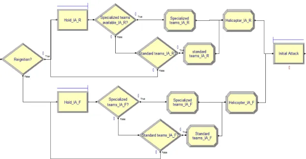
Figure 2 - Diagram of the suppression system developed. ... 16

Figure 3 - Modelling of PF arrivals; the same applies to FA. ... 18

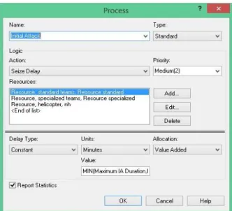
Figure 4 - Modelling IA for PF and RKD, with the major difference of including EXPRT crews, which modified the system design. ... 19

Figure 5 - Expression with the priorities of resources for IA. ... 19

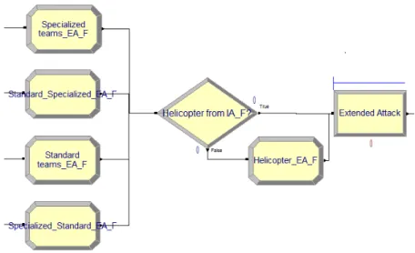
Figure 6 - "Process" module definitions for modelling IA, with 3 attributes representing different types of resources. ... 20

Figure 7 – Overview of complete EA modelling of NF and RKD. ... 20

Figure 8 - “Detail A” of Figure 7, from policy options with “Which policy_F?” module to the confirmation of the type(s) of resources available in “Combination available_EA_F”?, just for NF. ... 21

Figure 9 - "Detail B" of Figure 7, from the assignment of required resources to the corresponding attributes using 4 assign modules, to the execution of EA. ... 22

Figure 10 – Mapping for the complete fire rekindle probability modeling for STD and EXPRT crews (Appendix B, Figure 12). ... 24

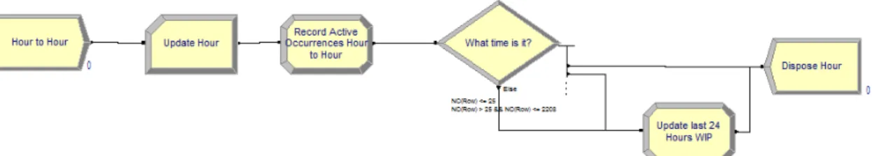
Figure 11 – Modeling the active events in the past 24 hours, with an entity “hour” created every hour. ... 25

Figure 12 - Complete modelling of the patch until a fire rekindles. ... 54

Figure 13 - Complete FA modelling. ... 55

Figure 14 - Complete FFA modelling. ... 56

Figure 15 - Suppression system developed in (Pacheco, Claro, and Oliveira 2013). ... 57

Figure 16 - Class "A" and Class "B" days of season. ... 58

Figure 17 - Distribution of the delay until a fire rekindles. ... 58

List of graphs

Graph 1 - Plots of values and fitted values for Porto (Pacheco, Claro, and Oliveira 2012). ... 22

Graph 2 - Evolution of RKD with 100% of STD crews. ... 27

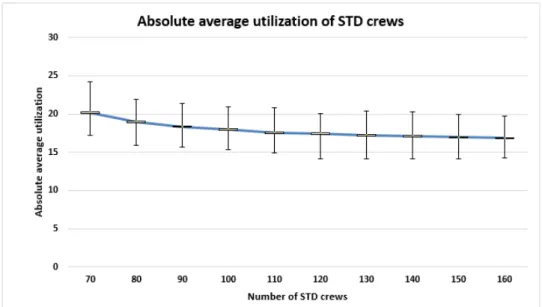
Graph 3 - Absolute average utilization of STD crews. ... 28

Graph 4 – Absolute maximum utilization of STD crews. ... 29

Graph 5 - Maximum WIP with PF, RKD, FA, and FFA included, at a given time. ... 30

Graph 6 - Evolution of the RKD taking into account different training levels, fixing 100 STD crews. ... 30

Graph 7 - Evolution of RKD setting STD crews training level in K=1/0.7/0.4/0.1, while covering the range 70-160. ... 31

Graph 8 - Evolution of RKD setting 70/100/160 STD crews, while covering the range of K in [1; 0.1]. ... 31

Graph 9 - Evolution of RKD fixing the number of crews at 80-20 (STD – EXPRT), while covering the probability to rekindle using EXPRT crews in the range of p in [10%,1%]. . 32

Graph 10 - Evolution of the RKD fixing 80%/20% STD/EXPRT crews and the probability to rekindle using EXPRT crews in 6%/3%/1%, while covering the range 70-160. ... 32

Graph 11 - Evolution of RKD with different number of EXPRT crews, from 0 to 100, and a 3% rekindle probability for each fire extinguished with those crews... 34

Graph 12- Evolution of RKD fixing EXPRT crews as 20%/40%/60%/80% of the total, within the range 70-160. ... 34

Graph 13 - Different policies to dispatch STD and EXPRT crews, fixing 20% of EXPRT crews with a 3% probability to rekindle whenever they are used. ... 35

Graph 14 - Different policies to dispatch STD and EXPRT crews, fixing 20% of EXPRT crews with a 6% probability to rekindle whenever they are used. ... 36

Graph 15 - Resources divided by classes and by IA/EA. ... 57

Graph 16 - Share of the burnt area and the number of fires in Europe southern countries, 2010. ... 58

List of tables

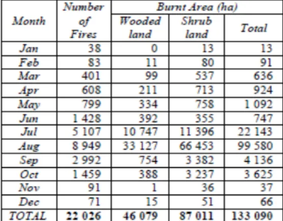
Table 1 - Number of fires and burnt area in Portugal (2010) distributed over 12 months

(Schmuck et al. 2011). ... 12

Table 2 - Parameters used to build more detailed graphs, such as Graph 2 or Graph 3. Each column stands for a different total of crews (in the range 70-160), and the rows represent the parameters required to build those graphs. ... 13

Table 3 – Some (not all) control variables used to calibrate the system; “Num Reps” – Number of replications; “standard teams” – Number of STD crews chosen; “specialized teams” – Number of EXPRT crews chosen; “helicopter” – Number of helicopters chosen; “Probability specialized teams” – Probability to rekindle whenever EXPRT crews are used; “K” – Training level of STD crews. ... 14

Table 4 – Sample of the responses (outputs) generated from the simulation. ... 14

Table 5 - Adjusting slope according to the total number of crews; on the left we have the new slopes adjusted to 100 crews and 200 crews; on the right, the relations between the number of crews and the number of active fires, with a linear trend. ... 23

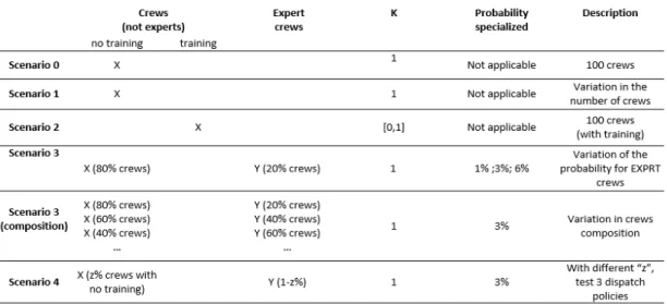
Table 6- Scenarios considered to test the SM, supported by the existence of two types of resources, besides the inclusion of training for STD crews; “K” – Parameter that controls rekindles quotient intensity (and simultaneously training level), varying between 0 and 1 (k*(A/R)), where it is better to have a smaller “K”; “Probability specialized” – probability of a fire to have a bad mop-up (fixed value) whenever fought with EXPRT crews. ... 26

Table 7 - Corresponding values of Graph 3. ... 28

Table 8 - Corresponding values of Graph 4. ... 29

Table 9 - Corresponding values of Graph 10. ... 33

Table 10 - Corresponding values of Graph 11. ... 34

Table 11 - Corresponding values of Graph 12. ... 35

Table 12 - Alternatives to reduce RKD to lower values, namely 10%, 25%, and 50%, considering different scenarios. ... 37

Table 13 - Budget available for training STD crews and for the inclusion of EXPRT crews, on the basis of scenario 1. Edu Bdgt – Education budget available for training; K – training factor; p – EXPRT crew’s probability to rekindle. ... 38

Table 14 – Maximum EXPRT crew firefighter payment, per hour; EXPRT Bdgt (max) – budget available for hiring EXPRT crews; EXPRT-FF pay/h - EXPRT crew firefighter

payment per hour; p – EXPRT crews probability. ... 39

Table 15 - Important parameters considered in the next tables of costs, namely the current payment per hour of 1.88€ (to STD crews) and the assumed payment four times higher to EXPRT crews. ... 39

Table 16 - Total suppression system cost, assuming a payment four times higher for EXPRT crew firefighters (7.5€ instead of 1.88€, per hour). ... 40

Table 17 - Suppression system cost variation (%), compared with the actual system design (only STD crews). ... 41

Table 18 - Suppression system cost variation (%) versus today's cost (2,070,000 €). ... 41

Table 19 - Model parametrizations. ... 58

List of expressions

Expression 1 - All the possible combinations among STD and EXPRT crews used in “hold” module, namely EXPRT + EXPRT, STD + STD, STD + EXPRT, or EXPRT + STD, where the former represents only IA resources and the latter only EA resources. ... 21 Expression 2 - Probability to rekindle when just STD crews are used. ... 23

Abbreviations and Symbols

RKD Rekindle

PF/NF Primary Fire/New Fire

STD Standard

EXPRT Expert

FA False Alert

FFA False “False Alarm”

IA Initial Attack

EA Extended Attack

SM Simulation Model

WIP Work In Progress

ELAC Equipa Logística de Apoio ao Combate ECIN Equipas de Combate a Incêndios

Chapter 1

Introduction

1.1 Wildfires and rekindles

There are few natural phenomena with the scope and complexity of wildland fires and they can be a major threat for the prosperity and well-being of communities (Pacheco and Claro 2014; Van Wagner 1985). Highly unpredictable factors, such as weather, suppression performance, or fire behavior, spread, and effect should be considered in forest fire management issue. These are just some of the reasons why wildfires are a complex phenomenon. As a consequence, they can put homes and people at risk, kill animals, destroy our habitats and create significant economic losses due to the destruction of wood. As they are a serious problem, it is necessary to study them beforehand, and then action is required in order to mitigate their consequences.

For this purpose, we can develop and use decision support systems (DSS) to help us make better decisions, especially when we are in the presence of uncertainty. They aim to facilitate the programming, capitalize on the investment, and quantify the risk (Thompson and Calkin 2011).

Forest fire management based on economic models is grounded on a balance between cost and net value-change, i.e., the C+NVC concept (Mavsar, Cabán, and Farreras 2010). In addition to this main issue, due to limited budgets, human resources and equipment, forest managers must decide their most efficient distribution over different types of interventions such as prevention (within the community and fuel treatments) or suppression (Mavsar, Cabán, and Farreras 2010). It is important to emphasize that DSS have an important role in decision making, as a support role, but do not replace the experience and intuition of the decision makers (Martell 1982).

have to be made concerning the quantity of resources to allocate to each fire, or a priority has to be assigned to a fire scenario over others, due to the scarcity of resources. An early decision, even with little information, is fundamental for the initial attack (IA) (Collins 2012).

The effectiveness of a suppression system, given a fixed number of resources, will depend on the number of simultaneous fires. Thus any factor contributing to increase those fires is directly harmful. RKD are one of those factors. They come from a barely extinguished fire, i.e., a still latent fire, which normally is not directly visible without special tools to help find signs that the cause remains there. Latent heat, sparks or embers are causes that, when not wholly eliminated, and combined with the remaining fuel, can lead to a re-ignition (NWCG 2011). Mop-up involves eliminating all hot areas and removing burning material (Pacheco, Claro, and Oliveira 2012a). Providing the example of Portugal, due to ineffective mop-up operations, 2497 of the 17048 wildfires were RKD. It is important to underline that this stage can be extended for days or weeks (Martell 2007) and is also very costly (González-Cabán 1984).

1.2 Research questions

With this work we intend to expand the horizons for quantitative analysis of the inclusion of new strategies in suppression management. We place the emphasis on suppression and mop-up operations, namely to avoid that, for example, 200 PF can become an additional 100 fires.

Our research question is as follows: “Should we invest in training STD crews and/or hiring

EXPRT crews?”

We will answer the question after the presentation and analysis of the results in the discussion and conclusion chapters.

1.3 Work context

This work comes as a follow-up of Pacheco, Claro, and Oliveira (2014a), integrated in project FIRE-ENGINE - Flexible Design of Forest Fire Management Systems (Claro 2010), with a particular focus on suppression policies targeting RKD, and is supported by body of work performed previously, including statistical and simulation analysis, introducing improvements to the original simulation model. The introduction of new resources (type) reinforces a DSS perspective in the analysis, in the sense that it makes it possible to test alternative suppression policies and resource mixes (Pacheco et al. 2015). Knowing that non-value added forest fire suppression activities, such as RKD and false alarms have a significant impact on suppression resources (Pacheco, Claro, and Oliveira 2014b), we aim at minimizing that value, introducing other more capable fire-fighting resources or improving the current ones, always within the available budget. By reducing RKD, in most cases, the real impact is important, saving animals, human lives, houses, and the landscape and allowing the country, in general, to preserve wood, an important economic resource.

1.4 Dissertation structure

This introduction concludes with an outline of the topics of the next chapters. In the second chapter we present the literature review on forest fires at large, and highlight other methods applied to related problems. The third chapter describes the methods used and the origin of the data. In the fourth chapter we analyze, in a detailed way, the simulation model (SM) and the major blocks comprising it, giving greater detail to the improvements resulting from this dissertation. Chapter 5 presents the results obtained from the simulation analysis. In the sixth chapter we discuss the results and analyze the costs of different alternatives. The conclusion provides an overview of the work developed, including limitations and future work.

Chapter 2

Literature Review

Over the years, even though the expenditures with suppression and prevention have increased, the devastation due to forest fires has also enlarged (Minas, Hearne, and Handmer 2012). This upward trend is largely dependent on the higher temperatures and varying weather conditions related to climatic changes (Wotton, Martell, and Logan 2003). As the expenses continue to grow, policy makers search for methods to achieve higher economic efficiency and for that, they look at both market and non-market profits (Venn and Calkin 2011). Wildfire managers face challenging situations when they need to make decisions, regarding, in particular, limited resources, little time to act, too much uncertainty and conflict of aims (Martell, Gunn, and Weintraub 1998).

OPERATIONS RESEARCH (OR) methods can support forest managers in operating in this

unpredictable environment. More specifically, OR makes use of analytical techniques, namely mathematical modelling and simulation, to identify and explore the quite complex interactions between the most relevant entities – people, resources and environment – to help the decision-making process and the design and operation of systems (Altay and Green III 2006). Wildfire managers can also utilize data extracted from different locations such as geospatial databases, fire behavior and climatology models (Minas, Hearne, and Handmer 2012). These available data, combined with OR methods, can provide support to the forest manager.

In forest fire management, there is a considerable literature concerning the use of OR methods, describing this approach from a methodological perspective (Martell 2015). The earliest literature about OR methods is reviewed by Martell (1982). This included work between 1961 and 1981, and major updates were only made later, in 1998 (Martell, Gunn, and Weintraub 1998). Since then, and up to 2012, a new revision was conducted by Minas, Hearne, and Handmer (2012). A review of DSS based on economic models was performed by Mavsar, González Cabán, and Varela (2013), and DSS including uncertainty and risk were reviewed by Thompson and Calkin (2011) and Pacheco et al. (2015). The most recent reference is the review by Martell (2015) of DSS applied to prevention and suppression (including detection).

2.1 Methods to deal with complexity

2.1.1 Mathematical programming and heuristics

Mathematical programming consists in the optimization, either maximization or minimization, of a given and measurable objective, where the objective is delineated in the form of a mathematical function that gather a certain number of constraints to meet that desirable optimization (Hillier and Lieberman 2005). Forest fire managers have to make decisions that are linked to others and confront themselves with resourcing and other operational constraints (Minas, Hearne, and Handmer 2012). Mathematical programming includes linear programming, integer programming, non-linear programming and dynamic programming.

In LINEAR PROGRAMMING, there is an objective function and the constraints can be expressed as a linear combination of the decision variables. An example of that method is a LP model for allocating suppression resources for an already active fire, with the intention of retarding at the maximum the spread of the fire to protection areas, mainly inhabited buildings (Hof and Omi 2003).

INTEGER PROGRAMMING is suitable for modelling situations involving indivisible resources, “if” and “then” logical connections, and “yes” or “no” resolution (Wolsey 1998). Kirsch and Rideout (2005) used it to model the preparation plan for the IA. The goal was to deliver IA resources bearing in mind a certain number of fires defined manually. The main objective was to maximize the weighted area protected, within a certain budget, where weights are attributed in terms of protection priorities.

NON-LINEAR PROGRAMMING differs from linear programming in relation to the objective function and constraints, which are not linear. The suppression time needed and the probability to contain a wildfire are kinds of non-linear functions, which means that a small delay to send IA resources can trigger important fire losses (Martell 2015).

DYNAMIC PROGRAMING (DP) is an optimization method useful when successive decisions in time need to be made, in other words, the state of a system at a given point in time depends on the state of the system before (Hillier and Lieberman 2005). The major feature of DP is that the main concern is to achieve the intended objective and the path to follow or the decisions made have no real importance. In the end, the outcomes should be the same, whatever the circumstances. Taking the example of Wiitala (1999), he used a DP model to determine the most efficient combination of different IA available resources to dispatch to a fire.

Forest fire management embodies various entities (public and private) where each one has their own interests, namely reduce effects on public safety, private property and forest ecosystems and evidently cost minimization (Martell 2007). Regular prescribed fire, on the one hand can bring security to buildings, but at the same time can have a negative impact on biodiversity in a few ecosystems (Driscoll et al. 2010).

Thus, for handling multiple conflicting objectives, MULTI-OBJECTIVE optimization (MO)

exists, appropriate to deal with potential effects on non-market values (conservation of flora and fauna, water quality, air quality or cultural heritage ((Venn and Calkin 2011)) due to its quite difficult quantification (Minas, Hearne, and Handmer 2012). MO models contain more than one objective function to find a group of Pareto optimal solutions, where a solution is considered Pareto-optimal if no objectives can be upgraded without downgrading another objective (Minas, Hearne, and Handmer 2012).

2.1.2 Problem structuring methods

Unlike classic OR methods, that are suitable to handle well-structured problems which can be formulated by means of performance measures, constraints and relations between action and consequence, PROBLEM STRUCTURING METHODS (PSMs) are good to deal with wildfires and disaster management because these phenomena don’t have a defined structure and can be analyzed in many different ways, as they are susceptible to disagreement among specialists (Minas, Hearne, and Handmer 2012). EXPERT ELICITATION and DECISION CONFERENCING are illustrations on PSMs.

DECISION CONFERENCING is usually a 2-day event than joins decision-makers from several entities to discuss a given topic and assist decision-making (Minas, Hearne, and Handmer 2012). The objective is to develop a shared knowledge of the problem (French 1996). It could also be applied to wildfires, so that the stakeholders can dialogue and assist the recovery-phase planning (Minas, Hearne, and Handmer 2012).

EXPERT ELICITATION (EE) consists in interviews or surveys to “subject experts” with the purpose of combining all their answers based on their experience and background. In this way, it can be used to understand the reasons for agreement and disagreement among the experts and to facilitate learning and conversing (Gregory et al. 2006). Hirsch, Corey, and Martell (1998) used this technique to model the association between fire intensity, fire size and probability of containing a fire by a set of five to seven crews through IA.

2.1.3 System dynamics

SYSTEM DYNAMICS is suitable for complex systems, where components are bonded through

feedback loops, which means that small changes to the inbound components, can produce substantial effects on the entire system (Anderson 1999). The main attribute of this method is that it permits the non-linearity and feedback-loop frameworks like in the real-word (social and physical systems) (Minas, Hearne, and Handmer 2012). First of all, SD aims to show how the problem operates in reality and as a second goal it is used to test different policies and alternatives (Forrester 1994). In the presence of little data available (which means less detail), it’s frequent to contact the experts, through EE, to obtain that missing information.

2.2 Methods for handling uncertainty

2.2.1 Simulation

When wildfire managers need to make decisions, they often come across uncertainties about the outcomes. SIMULATION provides a valuable tool to represent real life behavior and is

used for testing different situations. When building the model, the modeller gains a better perception of the real system (Maidstone 2012). Before implementation, models must be validated to guarantee that they are faithfully according to the reality and produce credible outputs (Winston and Goldberg 2004). At present, there are three techniques employed in simulation: discrete event simulation, system dynamics, and agent based simulation.

DISCRETE EVENT SIMULATION (DES) is likely the most used technique. The processes are

represented as a sequence of discrete events and the entities (in our case, the entities are the forest fires which need to be extinguished) run across different states over time (Maidstone 2012). DES systems are usually represented as networks of queues and servers. Pacheco, Claro, and Oliveira (2014a) developed a DES model to analyze the impact of RKD and false alarms on forest fire suppression.

SYSTEM DYNAMICS (mentioned in previous section) is a different approach from DES. It

focuses, not on individual behavior of the entities, but on flows around entities (Maidstone 2012). The main features taken into consideration are stocks, flows and delays. Stocks are stores of objects (for instance the number of patients in a hospital section), flows symbolize the movement of the items among different stocks in the system, as well as for outside/inside the system. A major aspect of SD is its ability to anticipate the system behavior through an analysis of the structure (Maidstone 2012). Collins (2012) developed an operational model to explore dynamics of occurrence of rekindled fires and Collins et al. (2013) applied SD to explore, through a strategic model, the impact of interactions between physical and political systems on the effectiveness of different assignments.

Another simulation method, although less used compared with DES and SD, is AGENT BASED

MODELING and consists in autonomous agents which follow a set of specified rules to reach

their objectives, at the same time interacting with each other and their environment (Maidstone 2012).

2.2.2 Stochastic programming

Stochastic programming is an approach for modeling optimization problems including uncertainty. While deterministic optimization problems are instanced with known values, real-world problems include unknown values at the moment when a decision has to be made (Shapiro and Philpott 2007). This technique models uncertain model parameters with known probability distributions or that can be estimated (Kall and Wallace 1994). Typically, the objective of stochastic programming is the optimization of the mean outcome or expected

system parameters are uncertain, which means that what they represent is true according to a given probability (Owen and Daskin 1998). To deal with uncertainty, other techniques, such as ROBUST OPTIMIZATION (Palma and Nelson 2009) and FUZZY MODELS (Iliadis 2005), can be applied.

2.3 Forest fire management research scope

Having identified the methods more commonly employed for handling complexity, including multiple conflicting objectives and uncertainty, and having illustrated them with some examples, now we can review the literature about DSS used in the prevention, detection and suppression (including IA and containment of a fire) of wildfires in particular and economic models currently used in different countries. Further ahead, to complete the literature review, we present recent research that aims to combine forest and fire management elements.

Unpredictable factors, such as weather forecasts, performance of suppression resources, and fire behavior, spread and effects, are essential aspects of the fire management and policy decisions. Theoretical and computational progress over the years has allowed an evolution of risk-based DSS to help decision making, namely facilitating a structured assessment of the outcomes and costs related to alternative strategies, budget, and a mix of suppression resources (Pacheco et al. 2015). These DSS may or may not represent economic models, depending on whether the objective is to minimize the costs (economic models) or to extinguish the fire as quickly as possible (knowing the expenses could be bigger).

2.3.1 Forest fire prevention

Prevention systems can be divided into within the community and fuel treatments. Their main purpose is to decrease fire incidence due to the human action, which is 98% (arson, negligence, or accidental) in Portugal (Pacheco, Claro, and Oliveira 2014a). The first one includes public campaigns and education and fuel treatments include prescribed burning and mechanical treatments, for example (Mavsar, Cabán, and Farreras 2010). Experts in prevention usually refer to the “three E’s of prevention”, namely engineering, education and enforcement (Martell 2015).

Currently, there are still very few updated revisions which make reference to the DSS that forest managers can use to help them understand how to best allocate their prevention resources to reduce human-caused fire occurrence, as well as few publications exploring the importance of the prevention enforcement. The early Heineke and Weissenberger (1974) work that makes reference to the outstanding discouragement policies hasn’t had the due development. Even so, the recent publications which handle the prevention in terms of engineering, are mostly about fuel management. Prestemon et al. (2010) have developed a statistical model, based on econometric methods, relating the human-cause fire occurrence to

a range of prevention measures, in Florida, and through a cost-benefit analysis of WPE (Wildfire Prevention Education) concluded that the gains outweigh the costs.

Finally, it’s important to clarify that these techniques applied to fire detection are not important in Portugal, because this is a country densely populated and their use makes sense in remote regions, uninhabited, and with low accessibility.

2.3.2 Forest fire suppression

Fire Detection is the stage that precedes the suppression and its point is to redirect fires to IA in the most efficient way possible, i.e, minimizing the time to act (still with small fires) and maximizing the effectiveness with the least costs possible (Martell 2015). The agencies adopt a mix of detection resources, for instance fixed lookout towers with digital cameras and a supervisor, satellites, detection patrol aircrafts and people that inform when passing over the places where a fire has ignited (Martell 2015). Therefore, it must be decided where to place the towers and the staff and where to send the detection patrol aircraft. Earlier research about this was made by Mees (1976), addressing tower location issues and by (Kourtz 1973) to approach the aerial detection patrol routing problem. More recently, there has been a growing interest in remote sensing and image processing systems respecting the fire detection. Mahdipour and Dadkhah (2014) revised wireless fire sensor network publications. Image processing by satellite sources by Benkraouda et al. (2014) and digital camera sources by Ko, Kwak, and Nam (2012) are other recent studies in the scope of detection.

Once a fire is detected, we enter the suppression stage. These two stages have a direct connection with each other, because the suppression always starts with detection. The bulk of the DSS and economic models developed aim at coping with active fires by means of IA to prevent them from becoming huge and uncontrollable (Fried and Fried 1996). IA consists in dispatching the first portion of resources to a fire, aiming to protect lives and material assets. It’s usually performed by ground and helitack crews. When a fire is not controlled by the IA, depending on the region or country, is classified as extended attack (EA), escaped fire or large fire. Giving the example of Ontario, when the IA is successful, is classified with the expression “Being Held”, which means that the duration, since the moment it was reported up to the moment it is contained, hasn’t exceeded twelve hours or its size is less than 4 ha (Martell 2015). In Portugal, since 2006, IA is performed by a crews with two engine crews, another vehicle with extra water supply, and, if available, a helicopter. The fire is delivered to EA and if not contained after the first 90 minutes, new resources will be dispatched (Pacheco, Claro, and Oliveira 2014a).

Some inherent decisions to the IA are the quantity of resources to dispatch onto a specific fire and when there are other concurrent fires, the need to distribute the few resources among them (Collins 2012) taking into account “the values at risk, fire behavior potential and many other factors” (Martell 2015). Those decisions have to be made promptly and under

Taking up some examples on the suppression issue we have the IA dispatch policy addressed by a deterministic integer linear programing (ILP) approach, done by Donovan and Rideout (2003) aiming to decide the best resources dispatching to a fire knowing it’s characteristics to minimize economic and non-economic losses from that fire. Later, Rideout, Wei, and Kirsch (2011) evolved previous Donovan and Rideout (2003) work to manage multiple fires, also as an ILP model. The model consists in dispatching IA resources from different bases, with a certain budget, with a day, a week or a fire season outlook, to minimize fire losses. Similarly, Hu and Ntaimo (2009) have also developed a model based on the research of Donovan and Rideout (2003) but designed a two-stage stochastic integer programming model. The objective was to dispatch resources to several fires, under uncertainty. These recent models represent new methods to the IA tough problem, but some of their assumptions prevent their use on the field (Martell 2015).

2.4 Economic models

The consideration of economic models seeks to find the most efficient distribution of a limited budget by prevention (education, public campaigns), fuel treatments (prescribed burning or mechanical treatments), pre-suppression (firefighters recruitment and training, maintenance of water points, and surveillance), and suppression. These models are typically based on the “cost plus net value-change” concept, C + NVC (Mavsar, Cabán, and Farreras 2010). LEOPARDS, KITRAL, and FPA are examples of such DSS.

LEOPARDS (Martell and Boychuk 1994, 1997) has been used in Ontario, Canada, since 1995 (McAlpine and Hirsch 1999a, 1999b). This system can model daily fire-suppression activities to assess IA performance under a diversity of policy and budget conditions (McAlpine and Hirsch 1999a). An early example of research on suppression is the IA simulation developed by (Martell et al. 1984) which makes use of temporal queuing conflicts and spatial realities (several fire ignitions in a small area and in a short time period or several fire ignitions in an extensive area (McAlpine and Hirsch 1999a, 1999b).

The Chilean system KITRAL (“fire” in indigenous Chilean language) has been in development since 1993, having started to be used in 1996. It was designed and constructed as a management support tool to reduce uncertainty and avoid assumptions, and can predict, across simulation models, fire behavior in many levels, such as risk, danger, fire model, spread rate, wind velocity, among other factors, via an extensive geographical database (Pedernera and Alvear 1999). KITRAL allows a daily allocation of resources considering their type and amount available for firefighting and also can make the strategic planning of activities (Pedernera and Alvear 1999).

FIRE PROGRAM ANALYSIS (FPA), applied in the U.S.A, was created after the severe wildfires in

would be to enable the agencies to coordinate their efforts and maximize their resources. This program would help fire agencies to weigh the benefits of fire suppression versus forest thinning, as well as to position people and equipment, and to decide on the number of airplanes to acquire. The system was supposed to be fine-tuned, calibrated and fully implemented in 2012. FPA was included on the 2014 federal budget (Pacheco et al. 2015).

Forest and fire management integration has been addressed by recent research to develop decision support tools. Those two aspects are often treated independently (Pacheco et al. 2015). Bettinger (2010) has discussed the potential of some techniques to strengthen the integration of forest and wildfire management elements. SADfLOR is a forest management DSS that emphasizes the key features needed to approach efficiently and effectively this integration between forest and fire management (Pacheco et al. 2015). SADfLOR was developed in Portugal with involvement of forest stakeholders, from Forest Services to forest industry, and including non-industrial forest owners (Pacheco et al. 2015). The base of the model incorporates growth and yield models for the most important Portuguese species and its methods include both precise and heuristic approaches to forest management planning (Garcia-Gonzalo et al. 2013).

Placing our work in the reviewed literature, as a DSS, it is capable of handling uncertainty by means of a simulation, and it also has an underlying economic model, with the introduction of different perspectives on the system cost. In the scope of forest fire research, it focuses on simulating a suppression system, in particular the dispatch of IA/EA resources to active fires.

Chapter 3

Data and Methods

3.1 2010 forest fires

The 2010 fire season was a relative unruffled year in Europe, but not for Portugal (by comparison), with an intense fire activity particularly in the first half of August, also heightened by meteorological conditions that affected fire spread. Among southern counties (Portugal, Spain, France, Italy, and Greece), Portugal was the most damaged, representing half of the fires and the burnt areas (Annex A, Graph 16). Despite this large portion, the total burnt area (133,090 ha in Graph 17) constituted about 87% of the average of the previous ten years (2000-2010), with 22,026 fires (Table 1). Concerning the fire season (July-September), it stands for 85% of all the occurrences (17,048) and 97% (125,859 ha) of the total burnt area of the entire year (Schmuck et al. 2011). Going deeper into the district of Porto, which is our case study, it features about 27% (6,007) of the total national forest fires, a considerable share, but a smaller burnt area percentage of 6.4% (8,551 ha) among all districts. Regarding RKD, they represented 11% of all real fires, or from a different perspective, 9.5% of all occurrences (including false alerts (FA) and false “false alarms” (FFA), described in Appendix A (page 49)). Table 1 - Number of fires and burnt area in Portugal (2010) distributed over 12 months (Schmuck et al. 2011).

3.2 Data source

All the data needed to develop the SM came from previous work, in which the focus was on statistical analysis. For more details, Pacheco, Claro, and Oliveira (2014a) should be consulted. Those data were pre-processed to characterize the following: the number of crews that were sent, in 2010, to IA and EA, as well as to PF/NF and RKD; the division in “Class A” and “Class B” days, based on the number of daily ignitions; the arrivals of PF, RKD, FA, and FFA, per hour, according to the class of the day, as well as their durations. In addition, we prepared a distribution of the time (delay) until a fire rekindles, from the data previously collected and processed.

3.3 Methods used

To develop the SM, described in detail in the next chapter, the Rockwell Arena simulation software was employed. This software uses a different way of programming, not with code (although it also allows that option), but visually, with specific blocks connected among them. It allowed the development of a model of a forest fire suppression system, to study the impact on RKD of different input parameters. We have also used Excel to build the graphs presented ahead.

Whereas Graph 1 plots single observations, other graphs, such as Graph 3 and 4, plot different statistics, namely those included in Table 2, for each scenario. For each point of the latter, we used individual values of all the 500 replications considered (each column of the previous table represents one point in the graph), from which we extracted maximum and minimum values. Other graphs may describe RKD, crew utilization, or other outputs. The number of observations corresponds to the 500 replications. To reach a final value for an Table 2 - Parameters used to build more detailed graphs, such as Graph 2 or Graph 3. Each column stands for a different total of crews (in the range 70-160), and the rows represent the parameters required to build those graphs.

“dpad” is the standard deviation of the observations. “alfa” is the significance level of the confidence interval. “HW” is the difference between the average and upper/lower bound of the interval, “Average +“/“Average –“ is the difference between the maximum/minimum and the average. The differences “Average – HW” and ”Average + HW” are displayed in the boxes featured in the graphs, and represent the 95% confidence interval for the mean. We used PAN (Process Analyzer) to have these data available from the simulations that we performed.

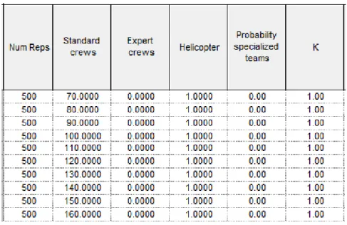
Table 3 shows the parameters that we can control (inputs) in order to influence the results (outputs) described in Table 4. The headers of these two tables represent the control variables and the responses, respectively.

Table 3 – Some (not all) control variables used to calibrate the system; “Num Reps” – Number of replications; “standard teams” – Number of STD crews chosen; “specialized

teams” – Number of EXPRT crews chosen; “helicopter” – Number of helicopters chosen;

“Probability specialized teams” – Probability to rekindle whenever EXPRT crews are used; “K” – Training level of STD crews.

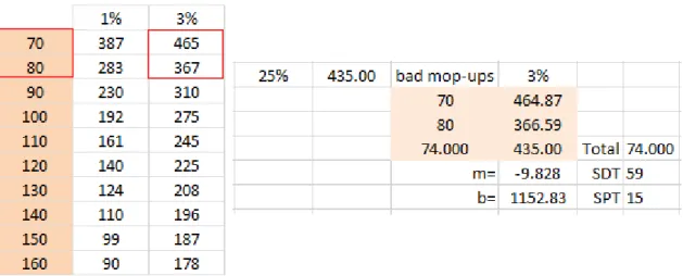
To conclude the presentation of the methods, to estimate the approximated combination of crews presented in Table 12 (page 37), we used interpolation with the two closer values. From Figure 1, and because 25% less RKD is a reduction from 580 to 435, we used 465 (rounded) and 367 (rounded), as highlighted above, because we know how many crews they correspond to and the target value is situated between them. This way, a linear interpolation using those two points allows us to find the value of 74 for the number of crews that correspond to 435 RKD.

Figure 1 – On the left are the highlighted values used on the interpolation on the right; as we know that 70 STD crews correspond to 464.87 RKD and 80 STD crews correspond to 366.59 RKD, we used the two points to find out the number of crews that correspond to 435 RKD, using linear interpolation.

Chapter 4

System design

4.1 Overview of the suppression system

As mentioned before, the suppression system considered in this work has as basis previous work, started with the dissertation of Pacheco (2011) and with its final version in Pacheco, Claro, and Oliveira (2014a). Some parts are identical, such as the statistical analysis and certain model blocks, representing well researched work that was an important background for this work. When quoting the previous work, namely the SM, the term “Colapsus v2.0” will be used, instead of the extended reference. Our own work is assigned the term “Colapsus v3.0”.

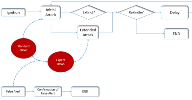
Figure 2 - Diagram of the suppression system developed.

In general, our model of the suppression system is not substantially different from the original. As shown in Figure 2, it is supplemented with EXPRT crews, a delay until a fire rekindles, and it does not include burnt area and losses due to forest fires. Although we

analyzed the impact of neither FA nor FFA, they are present in the SM, as they were important to make the results more precise and were part of “Colapsus v2.0”.

As a first higher-level explanation, when an occurrence is detected and depending on its type, which can be PF/NF (entering the system for the first time), RKD, FA or FFA, it is sent to IA and/or EA until it is extinguished. FA and FFA just have IA, corresponding to the time needed to discover that they are not real fires. On the other hand, PF go for IA and, if not eradicated within the defined time frame, are sent to EA. If the fire rekindles, after waiting a certain time, it effectively becomes an active RKD and follows the same sequence as a PF.

From here on, we will describe the different parts of our model in detail, giving priority to new features and omitting the details of “Colapsus v2.0”, which can be reviewed in detail in (Pacheco, Claro, and Oliveira 2014a).

4.2 Features implemented

The relevant parts we added to the model are the different types of resources that we can use, namely EXPRT crews, for which we can adjust the effectiveness before executing the SM. Another improvement, still in resources, is the possibility to provide STD crews with more or less training, through a parameter which affects directly the probability of a fire to rekindle.

We also improved the handling of the situations in which a fire can rekindle as a result of a previously extinguished fire. Before, they were autonomous entities entering the system in a schedule according to historical data. We now assign PF and RKD (the same fire can rekindle more than once) a probability to rekindle from its ancestor (the fire that originates a RKD), improving the accuracy to the model. Another feature implemented, although more discreet, is the inclusion of a delay (waiting time) until a fire rekindles, after its extinction. These are the upgrades we performed and will fully explain next.

4.3 Arrivals of NF, FA and FFA

We start the model description with the arrivals of NF (represented in Figure 3), FA, and FFA. NF and FA were divided in two classes of severity, “Class A” and “Class B”, with the former representing harsher wildland fires and days with more occurrences. FFA do not work with classes, so they enter the system normally, regardless of the class of the day. The “Fire Class.A” “create” module is used to create new entities. The “Accept NF” “decide” module is necessary to accept the entry of the entity in the system, if its class is equal to the class we assigned to the corresponding day, through the “CLS” variable (which contains the severity classes for the 92 days of the simulation), or to eliminate it from the system with the “dispose” module (which is not presented in the figure). The “entity” module owns five entities, namely NF/PF, FA, FFA, “Day”, and “Hour” (not included in “Colapsus v2.0”), the

system. The first three entities are managed by a schedule, while the last two are created one per day and one per hour, respectively. The RKD are not specific entities, but belong to a NF. When a NF re-ignites, we assign that entity a specific attribute, allowing us to know whether it is a RKD (or not). The “WIP” variable is used to count the active events in the system over time.

4.4 Initial Attack and Extended Attack

The approach to IA and EA remains mostly the same, but it involves an improvement in the option of dispatching EXPRT crews, besides STD crews (“Fire_Engine_Teams” in “Colapsus

v2.0”). Since 2006, in Portugal (Pacheco, Claro, and Oliveira 2014a), and in an ideal

situation, the resources dispatched to IA are two firefighting crews (ECIN – Equipa de Combate a Incêndios), three if an old vehicle is used (each crew with five elements), a supply vehicle with a driver and an assistant, called logistics crew to support the firefighting (ELAC – Equipa Logística de Apoio ao Combate) and even a helicopter (Pacheco, Claro, and Oliveira 2012b). In our work, the ECIN are called “STD crews” and the ”EXPRT” crews” are the fire brigades, known in Portugal as “bombeiros sapadores”. The IA/EA will be approached separately, because they operate differently.

In Figure 4, the “Reignition” “decide” module verifies whether the entity is a NF or a RKD (actually the entity type is a NF, but with an attribute called “Rekindled” which takes value 0 for NF and higher than 0 for RKD, depending on the number of times it has rekindled until that moment). Then, in a “hold” module entities wait for a given condition to become true, in this case the required resources – that are different for NF, RKD, FA, and FFA and even within each of them, depending on day class (Annex A, Graph 15) – becoming available. Next, the “Specialized teams_IA_F” “decide” module controls the resources to be dispatched, Figure 3 - Modelling of PF arrivals; the same applies to FA.

through priorities, including the policies that will be presented later. As the expression is too large to be included in the text, it can be seen in Figure 5 (below).

In case we do not choose a particular policy (“Policy number” variable with value 0

),

the system promptly chooses EXPRT crews whenever available; otherwise STD crews are always chosen through the next “decide” module “Standard teams_IA_F”. Generally, after the entities leave the “hold” module, one of those conditions has become true, but that may not be enough, since another entity could be facing the same situation at the same time, bringing the entity to the “process” module and waiting indefinitely for non-existing resources. As we cannot assume their existence (STD crews) when EXPRT crews are not available, that second “decide” module is critical to forward the entity to “hold” again. This solution is effective to describe this problem in the Arena software, and prevents the possibility described before. This was the default way chosen to assign the resources.

After this, two attributes, “Resource standard” and “Resource specialized”, get the value of the resources to be sent to IA. We also assign the attribute “nh” value “MR(helicopter) – NR(helicopter)”, zero or one, depending on the helicopter availability. The “Process” module properties (Figure 6) show how IA is treated, and we decided to keep the same module for NF and RKD. That is possible because each entity, whatever its type, knows beforehand the fire duration, through the “length” attribute, as well as “Maximum IA Duration”. Thus real IA Figure 5 - Expression with the priorities of resources for IA.

Figure 4 - Modelling IA for PF and RKD, with the major difference of including EXPRT crews, which modified the system design.

Once the IA has ended, if “length” is less than “Maximum IA Duration” (first “decide” of Figure 7), the fire does not go into EA and follows the first two paths (one is for NF and the other for RKD) of the module.

From now on we will describe the EA illustrated for NF. The next stage is to know which policy we are using (Figure 8, first “decide”; policy options: 0, 1, 2 or 3), following the first one (that can be 0 or 1).

Figure 7 – Overview of complete EA modelling of NF and RKD.

Figure 6 - "Process" module definitions for modelling IA, with 3 attributes representing different types of resources.

After this we check for EA resources, with EXPRT crews as the first option. If not available, the EA is paused and the crews coming from IA are freed. Actually, they are all released after IA (all the times) to avoid the internal problems already described, but because there is no waiting time ever since, when we do the verification we take into account all the resources (IA+EA) and no other entities seize them before this.

As shown in Figure 7, PF promptly goes into EA when one of the conditions from “Go now to extended attack_P1_F” is true, otherwise the entity proceeds to “Hold_EA_F” to wait for resources, where the first combination becoming available is immediately considered (now we need to assign IA and EA resources). After this, the “Combination available_EA_F” “decide” module checks which alternative “hold” was referring to (Expression 1).

The “else” path is once again important to safeguard against the possibility outlined when we described IA. If the resources needed really exist, the entity continues to one of the four “assign” modules (Figure 9, below), according to the previous “decide”. A new verification of the helicopter is made and the fire is ready to go into EA. The new duration is “length – Maximum IA Duration”. When the EA ends, “WIP” is decremented, and the entity is assigned a Figure 8 - “Detail A” of Figure 7, from policy options with “Which policy_F?” module to the confirmation of the type(s) of resources available in “Combination available_EA_F”?, just for NF.

Expression 1 - All the possible combinations among STD and EXPRT crews used in “hold” module, namely EXPRT + EXPRT, STD + STD, STD + EXPRT, or EXPRT + STD, where the former represents only IA resources and the latter only EA resources.

It is not entirely accurate that fires waiting for EA resources have no crews fighting them, but as in “Colapsus v2.0”, this gives us a margin to test the system with a lower collapse point, which represents the point (minimum value for the crews allocated) at which they start to be unable to perform the work accumulated, allowing RKD to increase indefinitely, and preventing the simulation from finishing.

4.5 Rekindles generated directly from NF

After a regression analysis for the 92 days of Charlie season in 2010, having Porto as a case study, relating the number of active fires on each day with the proportion of bad mop-ups, the results, published in Pacheco, Claro, and Oliveira (2012a) show a very consistent linear relation of these two variables, as we can see in Graph 1.

It is important to notice the evident linear growth of the proportion of bad mop-ups, with the number of active events each day (Pacheco, Claro, and Oliveira 2012a), so the pressure to attack other fires makes the combat to ongoing fires defective, allowing them to re-ignite later.

Graph 1 - Plots of values and fitted values for Porto (Pacheco, Claro, and Oliveira 2012). Figure 9 - "Detail B" of Figure 7, from the assignment of required resources to the corresponding attributes using 4 assign modules, to the execution of EA.

This analysis enabled the inclusion of RKD generated directly from NF or other RKD. The formula used to represent that probability is displayed in Expression 2. For each fire fought using one hundred percent of STD crews (for fires with EA or only with IA), a probability to rekindle is assigned based on the expression. Graph 1 does not represent any specific number of crews, being based only on the active events of each day and, from those events, the ones that rekindled later. The number of crews used is thus irrelevant, since we are only validating the model, and a calibration would be made according to the current number of crews chosen as the basis.

When looking at Table 5, if we parameterize the model for 100 STD crews, “New Slope” would be 0.05 and for 200 crews 0.1. So, dividing 0.1/200 or 0.05/100 we obtain the original slope (0.0005). When joining “New Slope”/”Total number of teams” in one variable, if we multiply this by the “Number of active fires”, the result would be the percentage of bad mop-ups” (as in the graph), here called “Probability to rekindle”. The “K” parameter represents the STD crews training level (1 – no training; 0 – maximum training and thus zero RKD). The “Factor” variable is used to calibrate RKD to be about 11%, otherwise we would obtain less than that percentage. Calculating this from historical data (Annex A, Table 20), “Factor” was assigned the value 2.2.

By simulation, and because the approach was not exactly the same, we got to 2.4. In place of considering daily active events (except FA and FFA), which was not possible because we do not know beforehand what will happen in the rest of the day, we considered, for each fire extinguished, the number of active ignitions in the past 24 hours. Even so, the difference is not substantial and it can be considered a good approximation.

After this theoretical explanation, we will now approach the modeling of the probability to rekindle. The “Fought by normal or specialized teams?” module is used to know which type of crews were used. If STD crews were used, their corresponding probability to rekindle is Table 5 - Adjusting slope according to the total number of crews; on the left we have the new slopes adjusted to 100 crews and 200 crews; on the right, the relations between the number of crews and the number of active fires, with a linear trend.

given by Expression 2. In the case of EXPRT crews, that probability is defined beforehand, with the chosen value defined between 0 and 10%. The fire rekindles if we obtain “1” from “DISC(Probability standard teams,1, 1.0, 0)” with STD crews or the same from “DISC(Probability specialized,1, 1.0, 0)” with EXPRT crews.

After this, the entity goes to the “store” module “Buffers to fire waiting to rekindle”, where the value of dormant fires is used in the control logic (section 3.7), and then goes to the “assign” and “delay” modules, the former specifically to generate the delay, and the latter where the fires wait to rekindle (the probability distribution of the delay is included in Annex A, Figure 17). Next, we increment the total number of RKD, the WIP, as well as the attribute “Rekindled” and the entity finally goes to the “unstore” module. After this, the re-ignition is activated and works exactly as a normal fire.

4.6 Modeling the active events in the last 24 hours

Behind the variable “Total 24 Hours” there is an expression and a set of assignments that make it possible to save those values for the entire simulation and apply them for each fire, regardless of the moment. All the modelling is displayed in Figure 11, except the storing of NF/RKD as they enter the system, which is done near the “create” module or when a fire rekindles.

In the beginning of each hour, the blocks in that figure are visited. The counter “NC(Row)” updates the current hour and the WIP is saved in the “WIP Recorder[NC(Row)]” vector. While hour is less or equal to 25, we just count the arrivals of NF or RKD, incrementing the vector “New Ignitions[NC(Row)]” and the variable “Total 24 Hours” by one (we do this every time one of those entities arrives into the system, as it belongs to another part of the model, just with an “assign” module right after each of them is created) and the Figure 10 – Mapping for the complete fire rekindle probability modeling for STD and EXPRT crews (Appendix B, Figure 12).

entity is disposed. When hour 26 is reached, older values need to be eliminated and new ones included, through the “Update last 24 Hours WIP” “assign” module. The most important expression of this part of the model is “Total 24 Hours - New Ignitions(i)+WIP Recorder(i+1) - WIP Recorder(i)”. Illustrating its application for hour 26 (the first that this module uses), we just subtract “New Ignitions(1)” and “WIP Recorder(2)” because it was more than 24 hours ago (about 25 hours) and we add “WIP Recorder(2)” because this interests us for being the active ignitions exactly 24 hours ago.

4.7 Control Logic

The control logic model is included in Annex A (Figure 18) and will not be presented here because it did not receive any modifications. The terminating conditions are defined in the Arena options. The first two conditions of “Day Counter >=92 && WIP == 0 && NSTO(Delay Storage)==0” keep unchanged from “Colapsus v2.0” and the third one is new, contemplating the situation in which fires are waiting to rekindle, preventing the simulation from stopping until the number of fires in the “storage” module falls to zero.

4.8 Model validation

The main difference regarding model validation is the inclusion of RKD as a result of previously extinguished fires, by means of a probability to rekindle. As mentioned before, we had only to adjust the “Factor” variable and obtained 2.4 by simulation (the theoretical value was 2.2). It is important to justify this difference and the first reason for it is the fact that we did not consider the active fires each day, but only in the past 24 hours. The second reason is the fact that we used simulation, which involves itself some uncertainty. Even so, the results are very reliable.

Figure 11 – Modeling the active events in the past 24 hours, with an entity “hour” created every hour.

Chapter 5

Results

Before the analysis of the results, we will describe the scenarios used to test the system. One important upgrade is the presence of EXPRT crews, allowing us to build a broader range of scenarios. Despite its simplicity, we considered the possibility of more training for STD crews, through a “K” training parameter, which allowed us to estimate the budget available to make the crews more capable and was included alone in the model (mixed with neither more highly trained STD crews nor EXPRT crews). In Table 6, as mentioned before (in chapter 4), we tuned scenario 0 for 100 STD crews.

The first scenario consists in the variation of STD crews, from 70 to 160. In the second scenario, with 100 fixed STD crews, we introduce training, using “K” to represent it, with values ranging from 1 (no training) to 0 (maximum training and no RKD). The parameter is multiplied by the probability to rekindle.

Table 6- Scenarios considered to test the SM, supported by the existence of two types of resources, besides the inclusion of training for STD crews; “K” – Parameter that controls rekindles quotient intensity (and simultaneously training level), varying between 0 and 1 (k*(A/R)), where it is better to have a smaller “K”; “Probability specialized” – probability of a fire to have a bad mop-up (fixed value) whenever fought with EXPRT crews.